Satellite isoprene retrievals constrain emissions and atmospheric oxidation

SUMMARY:

Isoprene is the dominant non-methane organic compound emitted to the atmosphere^1–3. It drives ozone and aerosol production, modulates atmospheric oxidation, and interacts with the global nitrogen cycle^4–8. Isoprene emissions are highly uncertain^1,9, as is the non-linear chemistry coupling isoprene and the hydroxyl radical, OH—its primary sink^10–13. Here we present the first global isoprene measurements from space, using the Cross-track Infrared Sounder (CrIS). These isoprene measurements, together with observations of its oxidation product formaldehyde, provide new constraints on isoprene emissions and atmospheric oxidation. We find that isoprene:formaldehyde relationships measured from space are broadly consistent with current understanding of isoprene-OH chemistry, with no indication of missing OH recycling at low-NO_x. We analyze these datasets over four global isoprene hotspots in relation to model predictions, and present a first demonstration of isoprene emission quantification based directly on satellite measurements of isoprene itself. A major discrepancy emerges over Amazonia, where current underestimates of natural NO_x emissions bias modeled OH and hence isoprene. Over southern Africa, we find that a prominent isoprene hotspot is missing from bottom-up predictions. A multi-year analysis sheds light on interannual isoprene variability, and suggests the role of El Niño.

Isoprene (2-methyl-1,3-butadiene), produced during photosynthetic metabolism and emitted mainly from leaves of woody plants, has global emissions comparable to those of methane and significantly greater than the sum of anthropogenic volatile organic compounds (VOCs)^1–3. Isoprene is highly reactive (lifetime <1 h at OH = 5 × 10⁶ molec cm⁻³) and plays a pivotal role in atmospheric oxidation, ozone, and aerosol formation^4–8. Air quality and chemistry-climate models thus require accurate isoprene emission inputs; however, current estimates span a wide range (~210–990 TgC y⁻¹ globally^1,9). Also uncertain is whether isoprene oxidation at low nitrogen oxide (NO_x) levels depletes versus sustains the abundance of hydroxyl radicals (OH)—the principal atmospheric oxidant^10–13. Space-borne measurements of formaldehyde (HCHO, an isoprene oxidation product) can provide top-down constraints¹⁴, but alone its use as an isoprene proxy is hampered by uncertainties in the NO_x-dependent chemistry governing the formaldehyde production yield and timescale¹⁵, and by competing non-isoprene formaldehyde sources^14,16–18.

Fu et al.¹⁹ recently demonstrated the viability of direct space-borne isoprene retrievals using infrared (IR) radiance measurements from the Cross-Track Infrared Sounder (CrIS). That study employed optimal estimation (OE) to retrieve isoprene column abundances (Ω_isoprene; Supplementary Note I; Supplementary Fig. 1) over Amazonia, with results validated using aircraft measurements. Here, we build on that work to develop an artificial neural network (ANN)-based algorithm for deriving global isoprene columns from CrIS. The ANN computational efficiency allows fuller exploitation of the dense CrIS sampling (~9×10⁶ spectra/day) for understanding spatial and temporal drivers of atmospheric isoprene. We thus derive the first global observations of atmospheric isoprene from space, and use this dataset to evaluate current understanding of its emissions and atmospheric oxidation.

Isoprene spectral index

As described in Methods, we use the CrIS-measured brightness temperature difference (ΔT_b) between the peak of the ν₂₈ isoprene band²⁰ and nearby off-peak channels (see Extended Data Fig. 1a) as a spectral index for deriving isoprene column abundances from the satellite data. Analogous methodologies have been used successfully for a range of other atmospheric species^21–24. Extended Data Fig. 1b shows the ΔT_b-isoprene relationship as simulated by a forward radiative transfer model for diverse conditions spanning the global atmosphere over land (Methods). The relationship is approximately linear with slope varying as a function of thermal contrast (atmosphere-surface temperature difference; Methods and Extended Data Fig. 1c). Interfering species likewise play a role and need to be accounted for as discussed later.

Figure 1 maps the global and seasonal ΔT_b distribution measured by CrIS. Clear enhancements are seen over many predicted isoprene source regions: Amazonia, northern Australia (January), central Africa (April), and the US Southeast (July). However, ΔT_b enhancements also manifest over regions not predicted by the GEOS-Chem chemical transport model (CTM; Methods) to have large isoprene sources (e.g., equatorial eastern Africa and the Arabian Peninsula, Pakistan and the US Southwest in July, Angola/Zambia in January and April). Elevated ΔT_b values also occur across the tropics, with spatial distribution resembling that of water vapor. As will be seen, ΔT_b enhancements not associated with high modeled isoprene can reveal locations where emissions are much higher than presently thought—many parts of the world lack flux measurements for regionally important plant species. However, we show later that the rest of these anomalous features disappear once thermal contrast, water vapor, and related factors are properly accounted for via the ANN.

Fig. 1 |. Global distribution of brightness temperature differences (ΔT_b) and isoprene columns.

Left column: monthly-mean ΔT_b observations from CrIS. Middle column: isoprene column densities derived from the CrIS observations. Right column: isoprene column densities simulated by GEOS-Chem. Data are plotted for January, April, July, and October 2013 at ~1330 LT (1200–1500 LT mean, with daily cloud screening applied). Ocean scenes are excluded from the isoprene maps as they are not part of the ANN training dataset (see Methods).

ANN-based isoprene measurements

We use a supervised feedforward ANN to derive isoprene columns from the CrIS ΔT_b data and contemporaneous observations of relevant surface and atmospheric properties (Methods). The employed ANN (representing the mean of 10 networks) reproduces 93% of the isoprene column variance across the full training data set. Prediction uncertainty is typically <30% for elevated isoprene columns (>1×10¹⁶ molec cm⁻²), increasing to 50% or more for low isoprene amounts/low thermal contrast.

We apply the trained ANN to the space-borne CrIS ΔT_b measurements to derive global isoprene distributions for January, April, July, and October 2013 (Methods). Because the statistical performance of the ANN summarized above does not necessarily represent the full observational uncertainty, we further evaluate our results with the previously validated OE retrievals¹⁹ and with independent aircraft measurements from two campaigns over the US Southeast^25,26.

Figure 2a compares the ANN and OE isoprene measurements over Amazonia for September 2014, revealing strong agreement between the two (r = 0.9, m = 0.8). Furthermore, Figure 2b shows that the aircraft-model comparisons (see Methods) yield slopes (m = 1.2–1.3) and correlations (r = 0.5–0.7) that statistically match the CrIS-model comparison (m = 1.3, r = 0.6), thus providing indirect validation of the CrIS data. The aircraft measurements also reveal key spatial features that are consistent with CrIS but not captured by GEOS-Chem. In particular, the largest observed isoprene enhancements occur over the Missouri Ozarks, farther north than model predictions—as also seen by CrIS. Finally, the enhancement magnitude measured during both aircraft campaigns is larger than predicted by the model, a finding likewise obtained from the CrIS data (Fig 2b).

Fig. 2. |. Comparison of the CrIS artificial neural network (ANN) isoprene columns with other datasets.

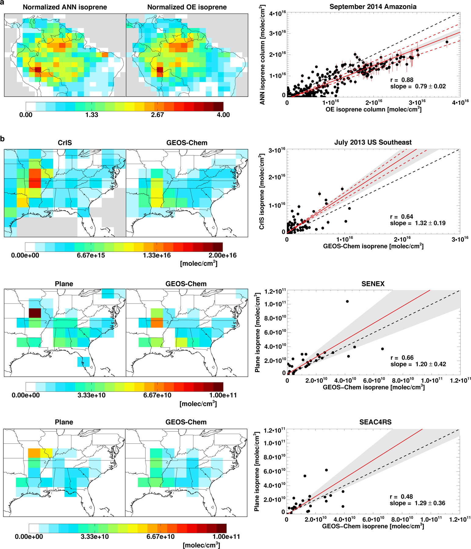
a, Comparison of ANN- and optimal estimation (OE¹⁹)-derived isoprene estimates. Both are derived from cloud-screened CrIS radiances for September 2014; ANN results employ GEOS-Chem HNO₃ as CrIS HNO₃ data were unavailable for this timeframe. The maps display columns normalized to their domain means, with the scatterplot comparing the absolute columns (absolute columns are mapped in Extended Data Fig. 2). b, Evaluation of CrIS ANN isoprene measurements using aircraft observations and GEOS-Chem model output. Top row: monthly-mean July 2013 isoprene columns as measured by CrIS (~1330 LT) and simulated by GEOS-Chem (1200–1500 LT mean). Bottom two rows: ambient isoprene concentrations as measured during the SENEX (June-July 2013; middle row) and SEAC⁴RS (August-September 2013; bottom row) aircraft campaigns and simulated by GEOS-Chem along the flight tracks. Data are plotted as campaign-average density-weighted boundary layer number densities (P > 800 hPa). In both a and b, error bars indicate the standard deviation across the 10 ANN-based columns (see Methods), red dashed lines indicate the range in slopes across ANNs, and black dashed lines indicate the 1:1 relation. Stated slope uncertainties and gray shaded regions represent the bootstrapped standard error of regression.

These results provide robust support for the ANN-derived isoprene abundances from CrIS. Looking forward, more validation datasets in high-isoprene regions (specifically, airborne or surface-based column measurements) would enable more extensive uncertainty assessment and retrieval improvement.

CrIS isoprene: links to emissions, OH

The global isoprene column distribution is governed by the balance between emissions and loss (predominantly via reaction with OH). Extended Data Fig. 3 maps global isoprene emissions, lifetimes, and columns predicted by GEOS-Chem. Because modeled OH (and therefore the isoprene lifetime) varies strongly with NO_x and with isoprene itself, the isoprene distribution differs substantially from that of emissions. For example, while predicted July emissions are higher in the US Southeast than Amazonia, the resulting isoprene columns are dramatically higher over Amazonia.

Figure 3a quantifies this effect in the model by plotting the global ensemble of monthly mean 1330 LT isoprene columns against emissions. Points are colored by simulated tropospheric nitrogen dioxide (NO₂), and two limiting regimes emerge. At elevated NO_x (Ω_NO2 ≳ 10¹⁵ molec cm⁻²) the relationship is near-linear, reflecting approximate local steady-state between isoprene columns and emissions—and slope corresponding to the isoprene lifetime. At lower NO_x, the isoprene columns increase superlinearly with emissions. In this regime (occurring in the model most notably over Amazonia) elevated isoprene suppresses OH and therefore its own sink, leading to runaway concentrations.

Fig. 3 |. Dependence of atmospheric isoprene columns on emissions and lifetime.

a, The global ensemble of monthly-mean ~1330 LT (1200–1500 LT mean) GEOS-Chem isoprene columns predicted for 2013 versus the corresponding isoprene emissions. b, The predicted isoprene:HCHO column ratio shown as a function of isoprene lifetime, 1/[OH], and [OH] (all for z < 500 m). Both plots are shaded by the modeled tropospheric NO₂ column.

Formaldehyde, an isoprene oxidation product, is more buffered to OH variability than is isoprene itself: i) photolysis ensures that HCHO removal continues even at low OH, and ii) its production is proportional to isoprene×OH, which is more stable than either quantity alone when elevated isoprene suppresses OH. Because of these differing sensitivities, the isoprene:HCHO column ratio is a proxy for the atmosphere’s oxidizing capacity over isoprene source regions. Figure 3b illustrates this relationship: on a global basis, across all locations and seasons, the monthly mean 1330 LT Ω_isoprene/Ω_HCHO ratios simulated by GEOS-Chem scale tightly with 1/[OH] (r = 0.94; Supplementary Note II discusses factors driving this relationship). A sensitivity analysis using an alternate isoprene oxidation mechanism (Mini-CIM⁸; see Methods) yields a similarly strong correlation (Supplementary Fig. 2), with details presented in Supplementary Note III.

The strong correlation in Fig. 3b encompasses the full global range of chemical regimes for isoprene oxidation: from unpolluted situations where isoprene-derived peroxy radicals (RO₂) are long-lived and react mainly with hydroperoxyl radicals (HO₂), other RO₂, or isomerize; to polluted areas where isoprene-derived RO₂ react quickly with NO^27,28. This globally aggregated Ω_isoprene/Ω_HCHO vs. 1/OH slope is weighted to isoprene-rich, OH-poor conditions: Supplementary Note III shows that the modeled slope varies across our analysis regions from 0.18 to 0.49. A sensitivity study with the independent Mini-CIM mechanism further shows systematic adjustments of 28 to 56% depending on location (Supplementary Fig. 4), while factors such as non-isoprene biogenic VOC emissions and model mixing assumptions (which influence the column-integrated OH-isoprene reaction rate²⁹) also influence the slope (Supplementary Note III). Overall, however, results here clearly demonstrate that the Ω_isoprene/Ω_HCHO provides a strong proxy of atmospheric oxidation that is observable from space.

We can therefore derive new constraints on isoprene:OH chemistry globally by combining the CrIS isoprene measurements derived here with space-based HCHO columns from OMI³⁰ (Ozone Monitoring Instrument; Methods). Specifically, we employ the measured isoprene:HCHO ratios from CrIS and OMI as a direct proxy of 1/[OH] (and hence the isoprene lifetime) that can be used to test chemical models. To that end, Fig. 4 plots the Ω_isoprene/Ω_HCHO ratios measured by CrIS + OMI and as simulated by GEOS-Chem. Data are shown as a function of isoprene and NO₂³¹ for months spanning all four seasons (Jan, Apr, Jul, Oct), and confined to scenes with elevated surface temperatures (>293 K) to limit noise due to low isoprene/thermal contrast. In both satellite-based and modeled relationships, we see a low-OH (and long isoprene lifetime) regime when isoprene is elevated and NO_x is low, and an opposing higher-OH (short lifetime) regime when the reverse is true. These oxidative regimes, and the chemical transitions between them, are generally consistent between model and observations, with the corresponding Ω_isoprene/Ω_HCHO ratios (and thus OH) agreeing to within 10–40% at low to moderate NO₂ (≲10¹⁵ molec cm⁻²). One clear discrepancy is that the model population of extremely high isoprene at extremely low NO_x is not seen in the data; as we will see this primarily reflects model NO_x errors over Amazonia. Some disparities also emerge at elevated NO₂; however, the observed values in this range have higher error due to limited measurements and lower isoprene columns with more uncertainty (Extended Data Fig. 4).

Fig. 4 |. Global distribution of the isoprene:HCHO ratio (a proxy for 1/OH; Fig. 3) as a function of isoprene and NO_x.

a, the observed relationship based on CrIS and OMI. b, the simulated relationship from GEOS-Chem. In both cases the plotted ratios represent monthly mean values at 1330 LT (1200–1500 LT mean) and are binned by isoprene and tropospheric NO₂ column amounts. Data shown reflect scenes with elevated surface temperature (> 293K at satellite overpass) and where the isoprene and HCHO measurements are above detection limit (2 × 10¹⁵ molec cm⁻²).

The above comparison supports the current model treatment of OH chemistry in the presence of isoprene. In particular, it argues against any substantial missing OH recycling at low NO_x^10,12,32—instead, the modeled OH levels are modestly higher than implied by the satellite data. A sensitivity analysis using the Mini-CIM⁸ isoprene oxidation mechanism supports this conclusion (Supplementary Note IV; Supplementary Fig. 5). In the following, we therefore examine the CrIS isoprene distribution and seasonality in light of the oxidative information provided by the Ω_isoprene/Ω_HCHO ratio, with measurement-model differences used to inform present understanding of emissions and atmospheric NO_x.

Figure 1 shows the global CrIS isoprene columns and corresponding GEOS-Chem predictions for January, April, July, and October 2013. The CrIS data reveal a number of isoprene hotspots that are consistent with the known isoprene sources discussed earlier—in particular, Amazonia, Central Africa, Australia, and the Ozarks of the US Southeast. These regions stand out because they combine strong emissions with a chemical regime where isoprene is sufficiently long-lived to be detectable from space (unlike, e.g., China in July, with elevated emissions but shorter isoprene lifetimes; Extended Data Fig. 3). For the months shown, the Central Africa and US Southeast enhancements peak in April and July, respectively, consistent with model predictions.

These dominant isoprene features are robust across the suite of ANN predictions: the column standard deviation across networks is typically <25% in these regions (Methods; Extended Data Fig. 5). The anomalous ΔT_b enhancements discussed earlier in the context of spectral interferences do not emerge as enhancements in the CrIS isoprene maps, showing that the ANN is effectively accounting for non-isoprene factors influencing ΔT_b. A notable feature not predicted by GEOS-Chem is the strong observed isoprene enhancement over southern Africa in January and, to a lesser degree, in April; this is explored further below.

Sections below examine each of the above hotspots in terms of their implications for present understanding of atmospheric isoprene. For each region we apply the corresponding Ωisoprene/ΩHCHO vs. 1/[OH] relationship in Supplementary Fig. 3 as a transfer function to quantify OH, and the isoprene lifetime, from the measured isoprene:HCHO ratios. The same transfer function is likewise applied to the model ratios (in this way, all relative model:measurement lifetime discrepancies arise solely from the underlying isoprene and HCHO column data, and are unaffected by any transfer function uncertainty). We further apply the satellite measurements to provide an initial quantification of isoprene (and NO_x) emissions over the same global hotspots, as detailed in Supplementary Note V and VI. From this analysis we identify and discuss emergent gaps in current bottom-up understanding of isoprene emissions. Results are summarized in Figs. 5–6 and in Supplementary Figs. 6–7 and 12–17.

Fig. 5 |. Seasonality of space-based isoprene over Amazonia and southern Africa.

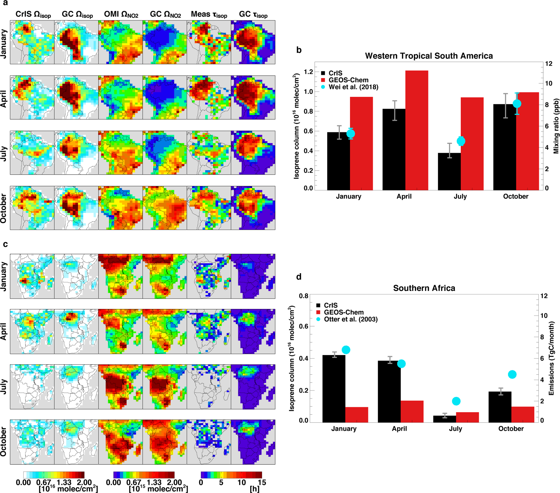
Left panels (a, c) map the CrIS and GEOS-Chem isoprene columns, OMI and GEOS-Chem tropospheric NO₂ columns, and space-based and GEOS-Chem isoprene lifetimes (τ_isop, calculated from the isoprene:HCHO ratios via the Fig. S3 transfer functions) for January, April, July, and October 2013. The CrIS isoprene and space-based isoprene lifetimes are shown for snow-free, above detection limit scenes (Ω_isoprene, Ω_HCHO > 2 × 10¹⁵ molec cm⁻²). Right panels (b, d) show the regional mean CrIS (black; error bars indicate the range across ANN predictions) and GEOS-Chem (red) isoprene columns for western South America (b, regions defined in Extended Data Fig. 6) and southern Africa (d). Results for western tropical South America are compared to in-situ mixing ratios (cyan points and error bars show the 1200–1500 LT mean and standard deviation) measured from May 2014-January 2015 in the central Amazon Basin³³. In-situ data were unavailable for most of July, so the July CrIS values are compared to the in-situ mean for June 2014. Southern Africa results are compared to monthly isoprene emissions from a detailed regional inventory⁴³.

Fig. 6 |. Seasonality of space-based isoprene over the US Southeast and Australia.

Left panels (a, c) map the CrIS and GEOS-Chem isoprene columns, OMI and GEOS-Chem tropospheric NO₂ columns, and space-based and GEOS-Chem isoprene lifetimes (τ_isop, calculated from the isoprene:HCHO ratios via the Fig. S3 transfer functions) for January, April, July, and October 2013. The CrIS isoprene and space-based isoprene lifetimes are shown for snow-free, above detection limit scenes (Ω_isoprene, Ω_HCHO > 2 × 10¹⁵ molec cm⁻²). Right panels (b, d) show the regional mean CrIS (black; error bars indicate the range across ANN predictions) and GEOS-Chem (red) isoprene columns for the US Southeast (b, regions defined in Extended Data Fig. 6) and southeast Australia (d). US Southeast results are compared to 10-year mean (1999–2008) isoprene concentration measurements from Atlanta, Georgia⁴⁸ (cyan; error bars indicate the 10-year standard deviation). Southeast Australian results are compared to measurements from the Sydney Particle Study⁴⁹. January and April CrIS values are compared to summer (1 February-7 March 2011) and autumn (14 April-14 May 2012) campaign means, respectively.

Amazonia

The CrIS isoprene columns over Amazonia reveal strong seasonal variability in both the magnitude and location of the isoprene maxima. For the months examined, observed columns in western South America (Fig. 5 bar plot; Extended Data Fig. 6) are highest in October and April and lowest in July. This is consistent with local ground-based measurements during GoAmazon³³, which exhibit a June minimum and increase nearly 2-fold from then to October (Fig. 5). Wei et al.³³ attribute this seasonal minimum to leaf-flushing between wet and dry seasons; other studies^34,35 also infer low isoprene emissions during new leaf growth in June-July. This seasonality is not well-represented in GEOS-Chem, which instead peaks in April and exhibits only a 5% July-October column increase.

Also apparent from Fig. 5 is that long isoprene lifetimes/low OH areas based on the Ω_isoprene/Ω_HCHO observations are also low-NO_x based on OMI NO₂ (e.g., Ω_NO2 < 0.2 × 10¹⁵ molec cm⁻² corresponds here in GEOS-Chem to surface [NO] < 32 ppt and RO₂ lifetimes to NO of >2.4 minutes), especially in January, April, and October. This agrees with chemical expectations for isoprene-rich, NO_x-poor environments, and thus provides strong confirmation of our approach, since the lifetime/OH constraints are derived only from isoprene and HCHO without incorporating any NO_x data.

Whereas the measured isoprene columns reveal localized maxima varying by season, GEOS-Chem instead predicts persistently elevated isoprene throughout much of western Amazonia. The model simultaneously predicts a much broader region of low OH (and elevated isoprene lifetime) than is inferred from the satellite data from January-July. We attribute these discrepancies mainly to the dramatic, widespread model NO_x underestimate apparent during these months (Fig. 5). While the modeled Amazonian NO_x levels are frequently low enough to yield the runaway isoprene concentrations discussed previously, the observations do not show this occurring to such an extent.

Simulations using the Mini-CIM mechanism (Supplementary Fig. 6), while featuring some spatial differences compared to the standard model, nonetheless lead to similar overall conclusions when evaluated against the satellite data. Specifically, predicted isoprene columns from January-July are higher than is observed, though to a lesser degree than in the base-case due to higher OH in Mini-CIM. Furthermore, the suppressed OH predicted by Mini-CIM over Amazonia extends over a broader geographic area than is revealed in the satellite data. As before, this disparity exhibits a spatial fingerprint matching the overly-low model NO_x as implied by OMI Ω_NO2.

The above Ω_NO2 bias could theoretically reflect model NO_x errors in the free troposphere or boundary layer^36,37; the former would have little effect on near-surface isoprene chemistry. However, we find that GEOS-Chem surface NO_x predictions are indeed significantly too low relative to surface observations during GoAmazon³⁸ (Supplementary Note V). Liu et al.³⁹ likewise infer from in-situ measurements a large near-surface NO_x bias in GEOS-Chem predictions for this region, which they attribute to underestimated soil emissions. Our satellite-based optimization described in Supplementary Note V (Supplementary Figs. 9–11; Supplementary Table 1) leads to substantial Amazonian NO_x emission increases that agree well with the Liu et al. findings.

Supplementary Fig. 11 further shows that our NO_x optimization successfully reduces the large isoprene lifetime biases over Amazonia in the prior model—providing independent confirmation of the results and supporting this first isoprene emission quantification using CrIS. We thus derive monthly Amazonian isoprene emissions that point to significant and coherent spatial errors in the bottom-up inventory (details in Supplementary Note V). Overall, these results highlight the critical need to better understand NO_x sources for this part of the world, and to elucidate the mechanisms driving isoprene emission variability in the tropics.

Africa

Two African isoprene hotspots are observed by CrIS: one in central Africa in April, and one in the Miombo and transitional woodlands of Angola peaking in January (Fig. 5)⁴⁰. While GEOS-Chem captures the timing of the central African enhancement, the CrIS data show the predicted isoprene peak to be too strong and too far north—as found previously based on OMI HCHO⁴¹ (model predictions using Mini-CIM are similar; Supplementary Fig. 6).

The Miombo/Angola peak has not been previously identified to this extent, though elevated leaf-level isoprene fluxes have been observed in woody savannas here⁴². Furthermore, while the CrIS-observed hotspot is largely missing from MEGANv2.1, it matches the location and season of highest emissions according to a regional inventory from Otter et al.⁴³ incorporating detailed local land-cover information. The enhancement location in a low-NO_x (and therefore low OH) area leads to large isoprene enhancements relative to the corresponding emissions and HCHO (Figs. 3, 5), explaining why a correspondingly strong HCHO peak is not seen. The CrIS seasonality over southern Africa also compares well with the Otter et al.⁴³ inventory (Fig. 5 bar plot; Extended Data Fig. 6), with a January maximum and July minimum. GEOS-Chem, conversely, peaks in April with isoprene columns 2–4× lower than CrIS.

The total isoprene emissions inferred from CrIS over southern Africa are higher than the prior estimate during January and April (Supplementary Fig. 13), and imply an emission overestimate north of the equator and underestimate to the south (particularly over Angola/Namibia). These emission adjustments broadly support previous HCHO-based findings^14,41,44,45. As described in Supplementary Note V, our CrIS-derived isoprene emissions for all of sub-equatorial Africa are highly consistent with the Otter⁴³ estimates, but substantially higher than MEGANv2.1. Such large discrepancies reveal a need for further investigation of isoprene sources in this understudied region.

US Southeast

CrIS isoprene columns over the US Southeast peak in July over the ‘isoprene volcano’ in Missouri/Arkansas, where surface mixing ratios up to 36 ppb have been observed⁴⁶. The aircraft data shown in Fig. 2b corroborate the CrIS isoprene distribution over this region, and OMI HCHO columns (Extended Data Fig. 7) likewise peak over the same part of the Ozarks during this time.

The GEOS-Chem isoprene maximum is shifted southward with lower column amounts than CrIS (Fig. 6; Supplementary Fig. 7). Kaiser et al.⁴⁷ emphasize the importance of correcting NO_x biases when inferring isoprene emissions, and indeed modeled NO₂ columns exhibit significant, spatially varying, biases over this region (Fig. 6, Supplementary Fig. 8). The isoprene lifetime predicted by the standard model is ~2× the satellite-inferred value over the southern portion of the domain (where model isoprene is biased high), and ~30–50% too low over Missouri (where the model is too low). However, the model does capture the observed regional isoprene seasonality⁴⁸ (Fig. 6). After correcting the NO_x biases above, we derive from the CrIS data moderate downward isoprene emission adjustments over Louisiana, Mississippi, and Alabama offset by increases over Missouri, Illinois, and eastern Texas (Supplementary Fig. 14).

Australia

CrIS isoprene columns over Australia are highest in the north during January and April, with smaller enhancements along portions of the eastern and southern coasts (Fig. 6). The northern Australia hotspot matches the location and timing of peak OMI HCHO (Extended Data Fig. 7). GEOS-Chem does not capture the observed spatial distribution, instead predicting peak enhancements over eastern Australia in January and weaker enhancements to the north and south (Fig. 6, Supplementary Fig. 7). As over the US Southeast, spatially varying NO_x biases are apparent and play a role in the above isoprene discrepancies.

Over southeastern Australia, the CrIS isoprene columns peak in January, with a ~25% decrease from January to April and a July minimum. GEOS-Chem predicts a much larger (~90%) January-April drop, with mean columns 40–95% lower than observed. In-situ measurements from the Sydney Particle Study⁴⁹ support the weaker seasonality seen by CrIS (Fig. 6). The CrIS-based source optimization shows that this modest seasonality also manifests in the underlying isoprene emissions (Supplementary Fig. 15).

Future outlook

We presented the first global picture of isoprene from space, derived from CrIS radiances using an artificial neural network (ANN). The reliability of the CrIS measurements is supported by comparisons to aircraft data and to (previously validated) optimal estimation measurements. However, more extensive validation data is needed to better quantify uncertainties and refine the measurement approach presented here.

Combining the CrIS measurements with contemporaneous HCHO observations provides a new space-based constraint on isoprene lifetimes, OH, and emissions. The satellite-derived isoprene:HCHO column ratios support current understanding of isoprene-OH chemistry as represented in GEOS-Chem. In particular, the satellite data provide no indication of substantial missing OH recycling under high-isoprene, low-NO_x conditions. A comparison between measured and predicted isoprene columns over key hotspot regions elucidates spatial and temporal biases in modeled isoprene emissions and NO_x, which highlight in particular the need for better mechanistic understanding of the drivers of tropical isoprene and NO_x sources.

Finally, this work lays a foundation for multi-year studies examining seasonal-to-interannual isoprene changes and their impacts on atmospheric chemistry. Supplementary Note VII illustrates this potential by applying the CrIS ANN retrieval from 2012–2018 over Amazonia and southern Africa (Supplementary Fig. 18). Results show that the strong seasonal patterns discussed earlier persist from year-to-year, but also reveal interannual differences tied to temperature shifts and climate features such as El Niño. Future analyses of the full global CrIS isoprene record can therefore elucidate key drivers of interannual ecosystem variability, including drought and other disturbance, and the couplings between climate, ecosystems, and atmospheric chemistry.

METHODS:

CrIS satellite sensor

CrIS is a Fourier transform spectrometer that was launched onboard the Suomi-NPP satellite in October 2011. A second CrIS instrument was launched onboard NOAA-20 in November 2017, and a third is planned for inclusion on JPSS-2 (expected launch in 2022). CrIS flies in a sun-synchronous orbit with 1330 LT daytime equator overpass. The early afternoon overpass is advantageous as it coincides with peak isoprene emissions⁵⁰ as well as with enhanced surface-atmosphere thermal contrast and vertical mixing—both of which increase the sensitivity of thermal IR sounders to near-surface absorbers. CrIS has an angular field of regard consisting of a 3 × 3 pixel array (each with a 14-km diameter nadir footprint) and a cross-track scan width of 2200 km, resulting in near-global coverage twice daily. The CrIS measurements have 0.625 cm⁻¹ spectral resolution in the longwave IR⁵¹, with noise characteristics (~0.04 K at 280 K) that improve significantly over other atmospheric sounders⁵². The high spectral resolution and low noise provide additional key advantages for measuring atmospheric isoprene.

GEOS-Chem simulation

We use the GEOS-Chem 3D chemical transport model (CTM) as an intercomparison platform for evaluating the isoprene estimates from CrIS, and to interpret the space-based observations in terms of isoprene emissions and chemistry. The model (v11–02e; www.geos-chem.org) employs GEOS-5 FP meteorological data from the NASA Global Modeling and Assimilation Office (GMAO), here regridded to 2° latitude × 2.5° longitude with 47 levels from the surface to 0.01 hPa. Simulations use a 10-min transport timestep (20-min for emissions and chemistry) and one-year initialization. Model output for 1200–1500 LT is used for comparison with the ~1330 LT CrIS and OMI observations.

GEOS-Chem includes detailed HO_x-NO_x-VOC-ozone-BrO_x chemistry coupled to aerosols^6,53. The v11–02e isoprene oxidation scheme^54–56 (which is consistent with the standard v11–02c mechanism detailed by Bates and Jacob⁸) has been extensively updated to reflect recent laboratory and field-based findings, in particular for the reaction of isoprene peroxy radicals (ISOPO₂) with HO₂⁵⁷ and isoprene epoxides with OH⁵⁸, ISOPO₂ self-reaction²⁷, aerosol uptake of isoprene oxidation products⁵⁵, and isoprene nitrate chemistry^54,59. ISOPO₂ isomerization^60–62 is treated explicitly, with oxidation and photolysis of the resulting hydroperoxyaldehydes following the current state-of-science^62–65 as described by Fisher et al.⁵⁴.

Along with base-case simulations using the standard (v11–02e) mechanism above, we perform sensitivity analyses using the Mini-CIM version of the reduced Caltech Isoprene Mechanism (RCIM^8,66), implemented in GEOS-Chem v11–02c. Mini-CIM is streamlined from the parent RCIM mechanism outlined by Wennberg et al.⁶⁶ by lumping very-low-yield (<0.1% globally) isoprene oxidation products to arrive at a number of organic species and reactions comparable to what is used in current global models. Bates and Jacob⁸ found global model results using Mini-CIM to be highly consistent with those using the more explicit parent mechanism (e.g., methane lifetime difference of < 0.1%), and thus recommend its use except in specialized applications involving highly functionalized, low-yield isoprene oxidation products.

An important feature of Mini-CIM is its dynamic treatment of the allylic and peroxy radicals resulting from the initial OH+isoprene addition^67,28 versus the fixed distributions used in prior mechanisms (including GEOS-Chem v11–02e). Mini-CIM also includes more intermolecular H shifts than older mechanisms, including rapid peroxy-hydroperoxy shifts^68,69 that increase low-NO OH recycling compared to GEOS-Chem v11–02e. An additional difference compared to our base-case simulations lies in the fact that Mini-CIM predicts more HCHO production at low-NO_x, with differences reaching approximately 20% for NO between 1 and 20 ppt⁸.

Biogenic emissions of isoprene and other VOCs are simulated using MEGANv2.1¹, implemented in GEOS-Chem as described by Hu et al.⁷⁰. Global anthropogenic emissions are based on the RETRO inventory for VOCs and on EDGARv4.2⁷¹ for NO_x, SO_x, and CO; each is overwritten by regional inventories over the U.S.⁷², Canada, Mexico⁷³, Europe⁷⁴, and Asia⁷⁵. GFED4⁷⁶ is used to compute biomass burning emissions; while lightning and soil NO_x emissions are from Murray et al.⁷⁷ and Hudman et al.⁷⁸, respectively.

Isoprene signal and brightness temperature difference

Isoprene has two IR absorption features (ν₂₇ and ν₂₈) in the vicinity of 900 cm⁻¹ that are associated with the wagging vibrational mode for each of the molecule’s =CH₂ groups²⁰. Extended Data Fig. 1a illustrates the radiance signal arising from those absorption features, plotted as the simulated difference in brightness temperature between an atmosphere with and without isoprene, assuming an isoprene profile with 5 ppb in the boundary layer and the US Standard Atmosphere for interfering species. Fu et al.¹⁹ demonstrated previously that the ν₂₇ and ν₂₈ features shown in Extended Data Fig. 1a are detectable from individual CrIS spectra over high-isoprene regions.

We start here from single-footprint Level 1B CrIS radiances that have been subsetted (1 of each 3 × 3 pixel array; FOV 6), cloud screened, and gridded to 0.5° latitude × 0.625° longitude. The ΔT_b values are then calculated as the difference between off-peak (mean of the spectral points at 894.375 and 895 cm⁻¹) and on-peak (mean of the spectral points at 893.125 and 893.75 cm⁻¹) T_b values at the ν₂₈ feature.

Cloud screening is based on the observed difference between the 900 cm⁻¹ brightness temperature and the surface skin temperature. We simulate this difference for clear-sky conditions as a function of water vapor column density (solid black line in Extended Data Fig. 8a) using the Line-by-Line Radiative Transfer Model^79,80 and employ a conservative linear approximation (solid red line in Extended Data Fig. 8a) to screen the observations. Temperature and water vapor information is from MERRA-2 reanalysis⁸¹ and interpolated to the time of CrIS overpass. We find good spatial correspondence between the location of our cloud-screened pixels and cloud flags derived from other spaceborne sensors such as VIIRS and MODIS.

Given the demonstrated importance of careful cloud screening for OE isoprene retrievals from CrIS¹⁹, we test the sensitivity of our results to cloud effects by employing a less stringent (by 2 K) brightness temperature threshold (dashed red line in Extended Data Fig. 8a). Results of this test are summarized in Extended Data Fig. 8b and c, and show that the resulting ΔT_b and isoprene changes are generally less than 15%, and less than 5% for enhanced isoprene levels. This suggests that the uncertainty in results presented here is not dominated by cloud effects.

Extended Data Fig. 1a shows that other atmospheric species (specifically water vapor, nitric acid, ammonia, and CFC-12) also have absorption features in the vicinity of the ν₂₇ and ν₂₈ isoprene peaks. We specifically employ ν₂₈ in computing ΔT_b as it is the stronger of the two bands and less subject to such interferences. Nevertheless, variability in these other atmospheric species (and in factors such as surface-atmosphere thermal contrast, surface elevation, and satellite viewing angle) can still affect the ΔT_b-isoprene relationship¹⁹, and are therefore accounted for in the estimation process described in the following section.

While other biogenically-derived VOCs with terminal =CH₂ groups may also absorb in the vicinity of the isoprene peaks, Fu et al.¹⁹ showed that the relevant primary biogenic species (including monoterpenes) with published absorption cross sections have much weaker absorption signals (< 0.01 K) than does isoprene at ν₂₈. Since we focus here on isoprene hotspots, we assume such effects to be minor for our analysis. Relevant absorption cross-sections for key non-HCHO isoprene oxidation products (methyl vinyl ketone, methacrolein, isoprene hydroxyhydroperoxides) have not been reported, but available analogs indicate that their spectral impact is likewise minor for analyses here (Supplementary Fig. 19). See Supplementary Note VIII for further discussion.

Extended Data Table 1 shows spatial correlations between the resulting CrIS ΔT_b measurements and simulated isoprene columns from the GEOS-Chem CTM over key source regions. Here and below, all satellite-model comparisons reflect monthly mean values at the ~1330 LT CrIS overpass with daily cloud screening. Correlations span r = 0.43–0.72. For comparison, Hu et al.⁷⁰ report r = 0.5–0.7 between simulated and measured isoprene in the US Midwest. A model-aircraft comparison over the US Southeast yields similar correlations (below). The CrIS ΔT_b values thus spatially correlate with isoprene predictions over known source regions to a degree commonly found for model-measurement comparisons of isoprene itself.

ANN training and forward prediction

We describe here a supervised feedforward (i.e., non-cyclic) ANN⁸² to derive isoprene columns from the CrIS ΔT_b observations. The approach employs a multilayer perceptron with training via Levenberg-Marquardt backpropagation⁸³ to account for the interfering effects mentioned above based on contemporaneous observations of other relevant surface and atmospheric properties.

Given a set of input variables x (in our case, ΔT_b and related parameters summarized in Extended Data Table 2), an ANN can be used to approximate an output f(x) (in our case, Ω_isoprene) that depends on x in an unknown and possibly non-linear way. This approximation occurs via a transfer function, Y(W, x), where W represents the weights of the function Y.

The weights are determined here with a synthetic data set, constructed based on a full year of simulated radiances from the Earth Limb and Nadir Operational Retrieval (ELANOR) model⁸⁴, which also serves as the operational forward model for the Tropospheric Emission Spectrometer (TES). ELANOR model inputs include temperature and water vapor profiles (using assimilated meteorological data from NASA GMAO) and climatological non-isoprene trace gas profiles (from the MOZART CTM⁸⁵). Isoprene profiles are taken from daily mid-afternoon (1200–1500 LT) GEOS-Chem predictions with 100% (1σ) Gaussian noise applied. We then apply global sampling (afternoon overpass, following the along-track separation of measurements from the global sampling strategy of TES⁸⁶, land scenes only) to arrive at a representative input dataset of appropriate size for ANN training. Finally, the resulting radiances are simulated (using temperature-dependent isoprene absorption look-up tables) for 3 satellite viewing angles (selected randomly for each scene). The full synthetic dataset comprises ~165,000 simulated spectra, from which we compute ΔT_b as above.

We then train the ANN to predict isoprene column densities based on six predictors (each taken as a firm constraint): ΔT_b, water vapor column density (Ω_H2O), column nitric acid density (Ω_HNO3), thermal contrast (taken as the difference between the surface skin and 2-meter air temperature), surface pressure, and satellite viewing angle. Alternate ANNs accounting for additional potential interferents (such as CFCs and ammonia) were tested but ultimately discarded as they contributed little additional power to the isoprene predictions. No location-specific information is included in the training: the network thus describes the general, global relationship between ΔT_b, isoprene columns, and associated factors that is mechanistically defined by the underlying spectroscopy. This is a key distinction from OE retrievals which incorporate varying amounts of prior information depending on the scene-specific sensitivity.

We assessed multiple network architectures and found the best performance for a three-layer model containing two (6- and 3-neuron) hidden layers and one (single-neuron) output layer using hyperbolic tangent (sigmoid) and linear transfer functions, respectively. The training occurs on 10 random extractions of the synthetic data set (after clustering to ensure representative sampling across the full range of isoprene column densities), with each extraction subsetted for training (50%), validation (30%), and testing (20%). The validation subset is used to determine when training can cease, and the testing subset is used subsequently to independently confirm network performance. Output from the resulting 10 networks are then averaged to provide the final ANN prediction.

Finally, we apply the trained ANN to the space-borne CrIS ΔT_b measurements to derive global isoprene distributions for January, April, July, and October 2013. Temperature and water vapor data are taken from the MERRA-2 reanalysis⁸¹ and interpolated to the CrIS overpass time, while nitric acid column observations are from the CrIS CLIMCAPS⁸⁷ product. All input variables are cloud-screened as described above prior to calculation of the gridded (2° × 2.5°) 1330 LT monthly mean. Less than 1% of the employed input variables fall outside the range used for ANN training (none of which occur over isoprene source regions), confirming that our training set is well-generalized.

Unlike a conventional OE retrieval, the ANN-based approach does not provide an estimate of the measurement vertical sensitivity (i.e., averaging kernel) and associated uncertainty for every individual scene. However, the ANN training statistics provide a quantification of the overall network performance, and therefore of the expected uncertainties for isoprene column abundances inferred from CrIS data. We find here that the six-predictor ANN can reproduce 93% of the variance in the isoprene total columns across the full synthetic data set (Extended Data Fig. 8d). The performance of each of the 10 networks relative to the independent testing set is similar (r² = 0.92–0.93, slopes ~1.0). This explanatory skill is lost when ΔT_b is withheld from training (r² = 0.28; Extended Data Fig. 8e)—confirming that the ANN predictive power is driven by the isoprene spectral signal rather than by the ancillary variables.

The relative uncertainty of the ANN predictions varies as a function of both isoprene amount and thermal contrast (Extended Data Fig. 8f). For elevated isoprene columns (>1×10¹⁶ molec cm⁻²) the prediction uncertainty is typically less than 30%, even with very low thermal contrast. Uncertainty increases for lower isoprene amounts, exceeding 50% for columns below 2×10¹⁵ molec cm⁻², and for columns below 5×10¹⁵ molec cm⁻² at low thermal contrast (0–5 K; Extended Data Fig. 1c shows thermal contrast maps for Jan, Apr, Jul, and Oct). These can be considered limits of detection for the 1330 LT monthly-mean isoprene columns derived from CrIS.

The statistical performance of the ANN as summarized above does not necessarily represent the full uncertainty of the CrIS isoprene measurements, since other factors (e.g., cross-section or radiative transfer errors, uncertainties in ancillary datasets used for water vapor, temperature, and HNO₃, uncertainties in the vertical profiles of isoprene used to train the ANN, residual cloud impacts) may also contribute. We therefore evaluate the CrIS isoprene columns using i) the previously published and validated OE retrievals and ii) independent atmospheric measurements, as described below and in the main text.

CrIS evaluation via aircraft-model intercomparison

Direct evaluation of the CrIS isoprene measurements is difficult due to lack of either i) ground-based isoprene column observations in isoprene hotspot regions, or ii) a statistically sufficient ensemble of full airborne profiles over isoprene source regions at the satellite overpass time. Instead, we perform here an indirect validation (Fig. 2b) using measurements from two aircraft campaigns over the US Southeast: SENEX (Southeast Nexus; 27 May – 10 July 2013²⁵) and SEAC⁴RS (Studies of Emissions and Atmospheric Composition, Clouds and Climate Coupling by Regional Surveys; 1 August – 23 September 2013²⁶). In each case, we employ the GEOS-Chem model as an intercomparison platform to quantify the level of consistency between CrIS and the in-situ aircraft data. Since any model isoprene bias should manifest in a consistent way relative to independent observational datasets for the same region and time period, the consistency between the CrIS/GEOS-Chem regression and the aircraft/GEOS-Chem regression reflects the agreement between the CrIS and in-situ isoprene datasets^88,89.

To perform this intercomparison, we sample the model at the time and location of the aircraft measurements (which are restricted to ±2 hours from the CrIS overpass time). Results discussed in the main text are aggregated to the model resolution and averaged vertically for each campaign by calculating a density-weighted mean boundary layer (P > 800 hPa) number density for each latitude × longitude grid cell.

OMI HCHO and NO₂ data

We use here the Quality Assurance for Essential Climate Variables (QA4ECV) version 1.0 Level 2 HCHO product from the OMI satellite sensor^29,90. OMI is a near-UV-visible spectrometer onboard NASA’s EOS Aura satellite, which has an equator overpass time (1340 LT) close to that of Suomi-NPP. The HCHO slant column density is determined via fitting of OMI radiances and subsequently converted to vertical column densities using a modeled shape factor. The QA4ECV retrieval uses a single, extended fitting interval (328.5–359.0 nm), whereas the precursor BIRA HCHO retrieval employed a smaller window with prefits for O₂-O₂ and BrO slant columns. While the QA4ECV data have yet to be fully validated, recent work has demonstrated its improved performance over the earlier BIRA retrieval⁹¹. Zhu et al.⁹² previously found the BIRA v14 HCHO retrieval to exhibit a 12% low bias (with use of an accurate shape factor) relative to aircraft measurements, and subsequent analysis has supported these findings⁹³. We find here that a global QA4ECV versus BIRA v14 comparison for the timeframe of our analysis yields a slope of 1.1–1.4 (0.9–1.8 over our targeted subregions), and we therefore do not apply any bias correction to the QA4ECV HCHO data. Repeating our analysis using instead the bias-corrected BIRA v14 dataset (Supplementary Figs. 20–22) leads to no substantive differences in our core results.

Standard data processing and screening procedures are followed. We restrict the data to solar zenith angle < 70° and cloud fraction < 0.4. The OMI data is then gridded to the 2 × 2.5° GEOS-Chem resolution. For all comparisons the model is sampled according to the OMI HCHO observation operator (i.e. averaging kernel) at the time and location of the satellite overpass.

Tropospheric NO₂ column data are from the OMI QA4ECV v1.1 monthly NO₂ product^31,94. The QA4ECV retrieval employs updated NO₂ spectral fitting that accounts for liquid water absorption and includes an intensity offset correction³¹. This improves the quality of the product, particularly over clear-sky ocean scenes⁹¹. OMI QA4ECV tropospheric NO₂ columns exhibited good agreement (bias = −2% and root-mean-square difference = 16%) as compared to ground-based column measurements in China³¹. Comparisons in this work are performed with respect to monthly-mean GEOS-Chem tropospheric NO₂ columns sampled at the time of the satellite overpass, with no observation operator applied.

DATA AVAILABILITY:

The CrIS Level 1B data used in this work is publicly available at http://disc.gsfc.nasa.gov/datacollection/SNPPCrISL1BNSR_1.html. The isoprene column data employed in this work are available at https://doi.org/10.13020/v959-dr15. The airborne data are publicly available for SENEX at http://esrl.noaa.gov/csd/projects/senex/ and for SEAC⁴RS at http://www-air.larc.nasa.gov/missions/seac4rs/index.html. OMI QA4ECV HCHO and NO₂ data are publicly available at http://www.qa4ecv.eu/ecvs.

CODE AVAILABILITY:

GEOS-Chem model code is publicly available at www.geos-chem.org. The LBLRTM^79,80, which is used to calculate the molecular absorption look-up tables employed in ELANOR⁸⁴, is publicly available at http://rtweb.aer.com/lblrtm.html.

Extended Data

Extended Data Fig. 1 |. Simulated spectral signals near 900 cm⁻¹ for the CrIS sensor.

a, Brightness temperature (T_b) difference for simulated spectra with and without isoprene (black), nitric acid (red), ammonia (blue), and CFC-12 (yellow), and a 10% perturbation in water vapor (green). Red and blue arrows indicate the ν₂₈ on-peak and off-peak spectral points used to calculate ΔT_b. Simulations were performed with LBLRTM^79,80 for an isoprene profile with 5 ppb in the boundary layer (P > 800 hPa) that decays exponentially aloft, and AFGL US standard atmosphere profiles of temperature, water vapor, and nitric acid. b, Relationship between ΔT_b and isoprene column density, shaded by thermal contrast, for the full synthetic dataset used in this work. c, Global distribution of surface-atmosphere thermal contrast at the time of the CrIS overpass. Maps are derived from time-interpolated GMAO temperatures for January, April, July, and October.

Extended Data Fig. 2 |. CrIS isoprene measurements over Amazonia as derived using ANN- and OE-based approaches.

Data are shown for September 2014 and displayed as absolute columns.

Extended Data Fig. 3 |. Global distribution of isoprene columns, emissions, and lifetime as predicted by GEOS-Chem.

Predicted columns (left column), emissions (middle column), and lifetime (z < 500 m; right column) are shown at 1330 LT for January, April, July, and October 2013.

Extended Data Fig. 4 |. Statistical uncertainty in the global distribution of monthly mean isoprene:HCHO ratios as a function of isoprene and NO_x regime.

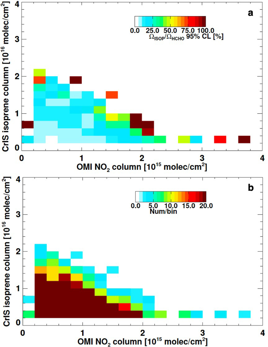
a, Relative 95% confidence interval in the mean ratio for each isoprene and tropospheric NO₂ bin. b, Number of observations in each bin.

Extended Data Fig. 5 |. Global distribution of isoprene column densities derived from CrIS.

Plotted are the mean (left column) and relative standard deviation (right column) across the 10 ANNs for January, April, July, and October 2013.

Extended Data Fig. 6 |.

Boundaries of the four regions examined in the seasonal bar plots shown in Figs. 5 and 6.

Extended Data Fig. 7 |. Measured and simulated HCHO columns.

Plotted are the HCHO columns measured by OMI (left column) and simulated by GEOS-Chem (right column) at ~1330 LT for January, April, July, and October 2013.

Extended Data Fig. 8 |. CrIS cloud screening and ANN performance.

a, Function used for cloud screening CrIS L1B data prior to ΔT_b calculation. The black line shows the modeled clear-sky difference between the 900 cm⁻¹ brightness temperature and surface skin temperature, as a function of water vapor column density (calculated using LBLRTM^79,80). The solid red line is the linear approximation used here, and the dashed red line represents a less stringent threshold used to test the sensitivity of the results to our cloud screening approach. Panels b and c show the sensitivity of the CrIS brightness temperature differences (b) and isoprene columns (c) to cloud screening. Data shown represent the median relative differences between the base-case results (derived using the solid red line panel a) and those derived using the less stringent cloud screening threshold (dashed red line in panel a). Scatterplots show the predicted versus true isoprene columns for (d) the six-predictor ANN and (e) an ANN in which ΔT_b is withheld as a predictor variable. Red dots show the mean of the 10 ANN predictions, and blue error bars show the standard deviation across the predictions. f, The relative uncertainty (based on the difference between the mean ANN predicted value and the true value) for the six-predictor ANN, binned as a function of thermal contrast and isoprene column density.

Extended Data Table 1 |.

Spatial correlation between monthly-mean CrIS ΔT_b and monthly-mean 1330 LT isoprene columns predicted by GEOS-Chem at 2° × 2.5° resolution for select regions.

Reqion	Month	ΔTb:GEOS-Chem isoprene correlation, r	# data points
Australia	January	0.54	323
Central Africa	April	0.43	357
US Southeast	July	0.72	90
Amazonia	October	0.57	340

Extended Data Table 2 |.

Data sources for the six input parameters used for ANN training and retrievals.

Input parameter	Source for training set	Source for ANN-based retrieval
ΔTb	ELANOR simulation	CrIS L1B radiances
H2O vapor column	Assimilated meteorology (GMAO; TES-like sampling)	Assimilated meteorology (GMAO; CrIS collocation)
HNO3 column	MOZART CTM	CrIS CLIMCAPS
Thermal contrast	Assimilated meteorology (GMAO; TES-like sampling)	Assimilated meteorology (GMAO; CrIS collocation)
Pressure	Assimilated meteorology (GMAO; TES-like sampling)	Assimilated meteorology (GMAO; CrIS collocation)
Satellite view angle	Randomly defined	CrIS satellite pointing angle

REFERENCES:

- 1.Guenther AB et al. The Model of Emissions of Gases and Aerosols from Nature version 2.1 (MEGAN2.1): an extended and updated framework for modeling biogenic emissions. Geosci. Model Dev 5, 1471–1492, doi: 10.5194/gmd-5-1471-2012 (2012). [DOI] [Google Scholar]
- 2.Saunois M et al. The global methane budget 2000–2012. Earth Syst. Sci. Data 8, 697–751, doi: 10.5194/essd-8-697-2016 (2016). [DOI] [Google Scholar]
- 3.Huang GL et al. Speciation of anthropogenic emissions of non-methane volatile organic compounds: a global gridded data set for 1970–2012. Atmos. Chem. Phys 17, 7683–7701, doi: 10.5194/acp-17-7683-2017 (2017). [DOI] [Google Scholar]
- 4.Trainer M et al. Models and observations of the impact of natural hydrocarbons on rural ozone. Nature 329, 705–707, doi: 10.1038/329705a0 (1987). [DOI] [Google Scholar]
- 5.Hewitt CN et al. Ground-level ozone influenced by circadian control of isoprene emissions. Nat. Geosci 4, 671–674, doi: 10.1038/ngeo1271 (2011). [DOI] [Google Scholar]
- 6.Mao JQ et al. Ozone and organic nitrates over the eastern United States: Sensitivity to isoprene chemistry. J. Geophys. Res.-Atmos 118, 11256–11268, doi: 10.1002/jgrd.50817 (2013). [DOI] [Google Scholar]
- 7.Lin YH et al. Epoxide as a precursor to secondary organic aerosol formation from isoprene photooxidation in the presence of nitrogen oxides. P. Natl. Acad. Sci. USA 110, 6718–6723, doi: 10.1073/pnas.1221150110 (2013). [DOI] [PMC free article] [PubMed] [Google Scholar]
- 8.Bates KH & Jacob DJ A new model mechanism for atmospheric oxidation of isoprene: global effects on oxidants, nitrogen oxides, organic products, and secondary organic aerosol. Atmos. Chem. Phys 19, 9613–9640, doi: 10.5194/acp-2019-328 (2019). [DOI] [Google Scholar]
- 9.Arneth A et al. Global terrestrial isoprene emission models: sensitivity to variability in climate and vegetation. Atmos. Chem. Phys 11, 8037–8052, doi: 10.5194/acp-11-8037-2011 (2011). [DOI] [Google Scholar]
- 10.Lelieveld J et al. Atmospheric oxidation capacity sustained by a tropical forest. Nature 452, 737–740, doi: 10.1038/nature06870 (2008). [DOI] [PubMed] [Google Scholar]
- 11.Fuchs H et al. Experimental evidence for efficient hydroxyl radical regeneration in isoprene oxidation. Nat. Geosci 6, 1023–1026, doi: 10.1038/ngeo1964 (2013). [DOI] [Google Scholar]
- 12.Feiner PA et al. Testing Atmospheric Oxidation in an Alabama Forest. J. Atmos. Sci 73, 4699–4710, doi: 10.1175/jas-d-16-0044.1 (2016). [DOI] [Google Scholar]
- 13.Rohrer F et al. Maximum efficiency in the hydroxyl-radical-based self-cleansing of the troposphere. Nat. Geosci 7, 559–563, doi: 10.1038/ngeo2199 (2014). [DOI] [Google Scholar]
- 14.Bauwens M et al. Nine years of global hydrocarbon emissions based on source inversion of OMI formaldehyde observations. Atmos. Chem. Phys 16, 10133–10158, doi: 10.5194/acp-16-10133-2016 (2016). [DOI] [Google Scholar]
- 15.Valin LC, Fiore AM, Chance K & Abad GG The role of OH production in interpreting the variability of CH2O columns in the southeast US. J. Geophys. Res.-Atmos 121, 478–493, doi: 10.1002/2015jd024012 (2016). [DOI] [Google Scholar]
- 16.Barkley MP et al. Net ecosystem fluxes of isoprene over tropical South America inferred from Global Ozone Monitoring Experiment (GOME) observations of HCHO columns. J. Geophys. Res.-Atmos 113, doi: 10.1029/2008jd009863 (2008). [DOI] [Google Scholar]
- 17.Zhu L et al. Anthropogenic emissions of highly reactive volatile organic compounds in eastern Texas inferred from oversampling of satellite (OMI) measurements of HCHO columns. Environ. Res. Lett 9, doi: 10.1088/1748-9326/9/11/114004 (2014). [DOI] [Google Scholar]
- 18.Boeke NL et al. Formaldehyde columns from the Ozone Monitoring Instrument: Urban versus background levels and evaluation using aircraft data and a global model. J. Geophys. Res.-Atmos 116, doi: 10.1029/2010jd014870 (2011). [DOI] [PMC free article] [PubMed] [Google Scholar]
- 19.Fu D et al. Direct retrieval of isoprene from satellite-based infrared measurements. Nat. Commun 10, 3811, doi: 10.1038/s41467-019-11835-0 (2019). [DOI] [PMC free article] [PubMed] [Google Scholar]
- 20.Brauer CS et al. Quantitative infrared absorption cross sections of isoprene for atmospheric measurements. Atmos. Meas. Tech 7, 3839–3847, doi: 10.5194/amt-7-3839-2014 (2014). [DOI] [Google Scholar]
- 21.Razavi A et al. Global distributions of methanol and formic acid retrieved for the first time from the IASI/MetOp thermal infrared sounder. Atmos. Chem. Phys 11, 857–872, doi: 10.5194/acp-11-857-2011 (2011). [DOI] [Google Scholar]
- 22.Clarisse L, Clerbaux C, Dentener F, Hurtmans D & Coheur PF Global ammonia distribution derived from infrared satellite observations. Nat. Geosci 2, 479–483, doi: 10.1038/ngeo551 (2009). [DOI] [Google Scholar]
- 23.Franco B et al. A General Framework for Global Retrievals of Trace Gases From IASI: Application to Methanol, Formic Acid, and PAN. J. Geophys. Res.-Atmos 123, 13963–13984, doi: 10.1029/2018jd029633 (2018). [DOI] [Google Scholar]
- 24.Whitburn S et al. A flexible and robust neural network IASI-NH3 retrieval algorithm. J. Geophys. Res.-Atmos 121, 6581–6599, doi: 10.1002/2016jd024828 (2016). [DOI] [Google Scholar]
- 25.Warneke C et al. Instrumentation and measurement strategy for the NOAA SENEX aircraft campaign as part of the Southeast Atmosphere Study 2013. Atmos. Meas. Tech 9, 3063–3093, doi: 10.5194/amt-9-3063-2016 (2016). [DOI] [PMC free article] [PubMed] [Google Scholar]
- 26.Toon OB et al. Planning, implementation, and scientific goals of the Studies of Emissions and Atmospheric Composition, Clouds and Climate Coupling by Regional Surveys (SEAC4RS) field mission. J. Geophys. Res.-Atmos 121, 4967–5009, doi: 10.1002/2015jd024297 (2016). [DOI] [Google Scholar]
- 27.Xie Y et al. Understanding the impact of recent advances in isoprene photooxidation on simulations of regional air quality. Atmos. Chem. Phys 13, 8439–8455, doi: 10.5194/acp-13-8439-2013 (2013). [DOI] [Google Scholar]
- 28.Teng AP, Crounse JD & Wennberg PO Isoprene Peroxy Radical Dynamics. J. Am. Chem. Soc 139, 5367–5377, doi: 10.1021/jacs.6b12838 (2017). [DOI] [PubMed] [Google Scholar]
- 29.Kim S-W, Barth MC, Trainer M Impact of turbulent mixing on isoprene chemistry. Geophys. Res. Lett, 43, 7701–7708, doi: 10.1002/2016GL069752 (2016). [DOI] [Google Scholar]
- 30.De Smedt I et al. Algorithm theoretical baseline for formaldehyde retrievals from S5P TROPOMI and from the QA4ECV project. Atmos. Meas. Tech 11, 2395–2426, doi: 10.5194/amt-11-2395-2018 (2018). [DOI] [Google Scholar]
- 31.Boersma KF et al. Improving algorithms and uncertainty estimates for satellite NO2 retrievals: results from the quality assurance for the essential climate variables (QA4ECV) project. Atmos. Meas. Tech 11, 6651–6678, doi: 10.5194/amt-11-6651-2018 (2018). [DOI] [Google Scholar]
- 32.de Gouw JA et al. Hydrocarbon Removal in Power Plant Plumes Shows Nitrogen Oxide Dependence of Hydroxyl Radicals. Geophys. Res. Lett 46, 7752–7760, doi: 10.1029/2019gl083044 (2019). [DOI] [Google Scholar]
- 33.Wei DD et al. Environmental and biological controls on seasonal patterns of isoprene above a rain forest in central Amazonia. Agr. Forest Meteor 256, 391–406, doi: 10.1016/j.agrformet.2018.03.024 (2018). [DOI] [Google Scholar]
- 34.Barkley MP et al. Regulated large-scale annual shutdown of Amazonian isoprene emissions? Geophys. Res. Lett 36, doi: 10.1029/2008gl036843 (2009). [DOI] [Google Scholar]
- 35.Alves EG et al. Leaf phenology as one important driver of seasonal changes in isoprene emissions in central Amazonia. Biogeosciences 15, 4019–4032, doi: 10.5194/bg-15-4019-2018 (2018). [DOI] [Google Scholar]
- 36.Silvern RF et al. Using satellite observations of tropospheric NO2 columns to infer long-term trends in US NOx emissions: the importance of accounting for the free tropospheric NO2 background. Atmos. Chem. Phys 19, 8863–8878, doi: 10.5194/acp-19-8863-2019 (2019). [DOI] [Google Scholar]
- 37.Rivas Belmonte et al. OMI tropospheric NO2 profiles from cloud-slicing: constraints on surface emissions, convective transport and lightning NOx. Atmos. Chem. Phys 15, 13519–13553, doi: 10.5194/acp-15-13519-2015 (2015). [DOI] [Google Scholar]
- 38.Martin et al. Introduction: Observations and Modeling of the Green Ocean Amazon (GoAmazon2014/5). Atmos. Chem. Phys 16, 4785–4797, doi: 10.5194/acp-16-4785-2016 (2016). [DOI] [Google Scholar]
- 39.Liu Y et al. Isoprene photochemistry over the Amazon rainforest, P. Natl. Acad. Sci. USA, 113, 6125–6130, doi: 10.1073/pnas.1524136113 (2016). [DOI] [PMC free article] [PubMed] [Google Scholar]
- 40.Guenther A et al. Isoprene emission estimates and uncertainties for the Central African EXPRESSO study domain. J. Geophys. Res.-Atmos 104, 30625–30639, doi: 10.1029/1999jd900391 (1999). [DOI] [Google Scholar]
- 41.Marais EA et al. Isoprene emissions in Africa inferred from OMI observations of formaldehyde columns. Atmos. Chem. Phys 12, 6219–6235, doi: 10.5194/acp-12-6219-2012 (2012). [DOI] [PMC free article] [PubMed] [Google Scholar]
- 42.Otter LB, Guenther A & Greenberg J Seasonal and spatial variations in biogenic hydrocarbon emissions from southern African savannas and woodlands. Atmos. Environ 36, 4265–4275, doi: 10.1016/s1352-2310(02)00333-3 (2002). [DOI] [Google Scholar]
- 43.Otter L et al. Spatial and temporal variations in biogenic volatile organic compound emissions for Africa south of the equator. J. Geophy. Res.-Atmos 108, doi: 10.1029/2002jd002609 (2003). [DOI] [Google Scholar]
- 44.Stavrakou T et al. Global emissions of non-methane hydrocarbons deduced from SCIAMACHY formaldehyde columns through 2003–2006. Atmos. Chem. Phys 9, 3663–3679 (2009). [Google Scholar]
- 45.Marais EA et al. Improved model of isoprene emissions in Africa using Ozone Monitoring Instrument (OMI) satellite observations of formaldehyde: implications for oxidants and particulate matter. Atmos. Chem. Phys 14, 7693–7703, doi: 10.5194/acp-14-7693-2014 (2014). [DOI] [Google Scholar]
- 46.Wiedinmyer C et al. Ozarks Isoprene Experiment (OZIE): Measurements and modeling of the “isoprene volcano”. J. Geophys. Res.-Atmos 110, doi: 10.1029/2005jd005800 (2005). [DOI] [Google Scholar]
- 47.Kaiser J et al. High-resolution inversion of OMI formaldehyde columns to quantify isoprene emission on ecosystem-relevant scales: application to the southeast US. Atmos. Chem. Phys 18, 5483–5497, doi: 10.5194/acp-18-5483-2018 (2018). [DOI] [Google Scholar]
- 48.Hansen DA et al. The southeastern aerosol research and characterization study: Part 1-overview. J. Air Waste Manage 53, 1460–1471, doi: 10.1080/10473289.2003.10466318 (2003). [DOI] [PubMed] [Google Scholar]
- 49.Emmerson KM et al. Current estimates of biogenic emissions from eucalypts uncertain for southeast Australia. Atmos. Chem. Phys 16, 6997–7011, doi: 10.5194/acp-16-6997-2016 (2016). [DOI] [Google Scholar]
- 50.Guenther AB & Hills AJ Eddy covariance measurement of isoprene fluxes. J. Geophys. Res.-Atmos 103, 13145–13152, doi: 10.1029/97jd03283 (1998). [DOI] [Google Scholar]
- 51.Han Y et al. Suomi NPP CrIS measuremets, sensor data record algorithm, calibration and validation activities, and record data quality. J. Geophys. Res.-Atmos 118, 12734–12748, doi: 10.1002/2013jd020344 (2013). [DOI] [Google Scholar]
- 52.Zavyalov V et al. Noise performance of the CrIS instrument. J. Geophys. Res.-Atmos 118, 13108–13120, doi: 10.1002/2013jd020457 (2013). [DOI] [Google Scholar]
- 53.Millet DB et al. A large and ubiquitous source of atmospheric formic acid. Atmos. Chem. Phys 15, 6283–6304, doi: 10.5194/acp-15-6283-2015 (2015). [DOI] [Google Scholar]
- 54.Fisher JA et al. Organic nitrate chemistry and its implications for nitrogen budgets in an isoprene- and monoterpene-rich atmosphere: constraints from aircraft (SEAC4RS) and ground-based (SOAS) observations in the Southeast US. Atmos. Chem. Phys 16, 5969–5991, doi: 10.5194/acp-16-5969-2016 (2016). [DOI] [PMC free article] [PubMed] [Google Scholar]
- 55.Marais EA et al. Aqueous-phase mechanism for secondary organic aerosol formation from isoprene: application to the southeast United States and co-benefit of SO2 emission controls. Atmos. Chem. Phys 16, 1603–1618, doi: 10.5194/acp-16-1603-2016 (2016). [DOI] [PMC free article] [PubMed] [Google Scholar]
- 56.Travis KR et al. Why do models overestimate surface ozone in the Southeast United States? Atmos. Chem. Phys 16, 13561–13577, doi: 10.5194/acp-16-13561-2016 (2016). [DOI] [PMC free article] [PubMed] [Google Scholar]
- 57.Liu YJ, Herdlinger-Blatt I, McKinney KA & Martin ST Production of methyl vinyl ketone and methacrolein via the hydroperoxyl pathway of isoprene oxidation. Atmos. Chem. Phys 13, 5715–5730, doi: 10.5194/acp-13-5715-2013 (2013). [DOI] [Google Scholar]
- 58.Bates KH et al. Gas Phase Production and Loss of Isoprene Epoxydiols. J. Phys. Chem. A 118, 1237–1246, doi: 10.1021/jp4107958 (2014). [DOI] [PubMed] [Google Scholar]
- 59.Jacobs MI, Burke WJ & Elrod MJ Kinetics of the reactions of isoprene-derived hydroxynitrates: gas phase epoxide formation and solution phase hydrolysis. Atmos. Chem. Phys 14, 8933–8946, doi: 10.5194/acp-14-8933-2014 (2014). [DOI] [Google Scholar]
- 60.Crounse JD, Paulot F, Kjaergaard HG & Wennberg PO Peroxy radical isomerization in the oxidation of isoprene. Phys. Chem. Chem. Phys 13, 13607–13613, doi: 10.1039/c1cp21330j (2011). [DOI] [PubMed] [Google Scholar]
- 61.Peeters J, Nguyen TL & Vereecken L HOx radical regeneration in the oxidation of isoprene. Phys. Chem. Chem. Phys 11, 5935–5939, doi: 10.1039/b908511d (2009). [DOI] [PubMed] [Google Scholar]
- 62.Wolfe GM et al. Photolysis, OH reactivity and ozone reactivity of a proxy for isoprene-derived hydroperoxyenals (HPALDs). Phys. Chem. Chem. Phys 14, 7276–7286, doi: 10.1039/c2cp40388a (2012). [DOI] [PubMed] [Google Scholar]
- 63.Peeters J & Muller JF HOx radical regeneration in isoprene oxidation via peroxy radical isomerisations. II: experimental evidence and global impact. Phys. Chem. Chem. Phys 12, 14227–14235, doi: 10.1039/c0cp00811g (2010). [DOI] [PubMed] [Google Scholar]
- 64.Stavrakou T, Peeters J & Muller JF Improved global modelling of HOx recycling in isoprene oxidation: evaluation against the GABRIEL and INTEX-A aircraft campaign measurements. Atmos. Chem. Phys 10, 9863–9878, doi: 10.5194/acp-10-9863-2010 (2010). [DOI] [Google Scholar]
- 65.Squire OJ et al. Influence of isoprene chemical mechanism on modelled changes in tropospheric ozone due to climate and land use over the 21st century. Atmos. Chem. Phys 15, 5123–5143, doi: 10.5194/acp-15-5123-2015 (2015). [DOI] [Google Scholar]
- 66.Wennberg PO et al. Gas-phase oxidation of isoprene and its major oxidation products. Chem. Rev, 118, 3337–3390, doi: 10.1021/acs.chemrev.7b00439 (2018). [DOI] [PubMed] [Google Scholar]
- 67.Peeters J et al. Hydroxyl radical recycling in isoprene oxidation driven by hydrogen bonding and hydrogen tunneling: the upgraded LIM1 mechanism, J. Phys. Chem. A, 118, 8625–8643, doi: 10.1021/jp5033146 (2014). [DOI] [PubMed] [Google Scholar]
- 68.Jørgenson S et al. Rapid hydrogen shift scrambling in hydroperoxy-substituted organic peroxy radicals, J. Phys. Chem. A, 120, 266–275, doi: 10.1021/acs.jpca.5b06768 (2016). [DOI] [PubMed] [Google Scholar]
- 69.Moller KH et al. The importance of peroxy radical hydrogen-shift reactions in atmospheric isoprene oxidation, J. Phys. Chem. A, 123, 920–932, doi: 10.1021/acs.jpca.8b10432 (2016). [DOI] [PubMed] [Google Scholar]
- 70.Hu L et al. Isoprene emissions and impacts over an ecological transition region in the US Upper Midwest inferred from tall tower measurements. J. Geophys. Res.-Atmos 120, 3553–3571, doi: 10.1002/2014jd022732 (2015). [DOI] [Google Scholar]
- 71.European Commission (EC): Joint Research Centre (JRC)/Netherlands Environmental Assessment Agency (PBL),Emission Database for Global Atmospheric Research (EDGAR), release version 4.2, http://edgar.jrc.ec.europa.eu, (2011).
- 72.EPA: 2011 National Emissions Inventory (NEI) data, http://www.epa.gov/air-emissions-inventories/2011-national-emissions-inventory-nei-data, (2015).
- 73.Kuhns H, Green M & Etyemezian V Big Bend Regional Aerosol and Visibility Observational (BRAVO) Study Emissions Inventory, DRI, Las Vegas, NV, (2003). [Google Scholar]
- 74.Auvray M & Bey I Long-range transport to Europe: Seasonal variations and implications for the European ozone budget. J. Geophy. Res.-Atmos 110, doi: 10.1029/2004jd005503 (2005). [DOI] [Google Scholar]
- 75.Li M et al. MIX: a mosaic Asian anthropogenic emission inventory under the international collaboration framework of the MICS-Asia and HTAP. Atmos. Chem. Phys 17, 935–963, doi: 10.5194/acp-17-935-2017 (2017). [DOI] [Google Scholar]
- 76.van der Werf GR et al. Global fire emissions estimates during 1997–2016. Earth Syst. Sci. Data 9, 697–720, doi: 10.5194/essd-9-697-2017 (2017). [DOI] [Google Scholar]
- 77.Murray LT et al. Optimized regional and interannual variability of lightning in a global chemical transport model constrained by LIS/OTD satellite data. J. Geophys. Res.-Atmos 117, D20307, doi: 10.1029/2012JD017934 (2012). [DOI] [Google Scholar]
- 78.Hudman RC et al. Steps towards a mechanistic model of global nitric oxide emissions: implementation and space-based constraints. Atmos. Chem. Phys 12, 7779–7795, doi: 10.5194/acp-12-7779-2012 (2012). [DOI] [Google Scholar]
- 79.Clough SA et al. Atmospheric radiative transfer modeling: a summary of the AER codes. J. Quant. Spectrosc. Ra 91, 233–244, doi: 10.1016/j.jqsrt.2004.05.058 (2005). [DOI] [Google Scholar]
- 80.Alvarado MJ et al. Performance of the Line-By-Line Radiative Transfer Model (LBLRTM) for temperature, water vapor, and trace gas retrievals: recent updates evaluated with IASI case studies. Atmos. Chem. Phys 13, 6687–6711, doi: 10.5194/acp-13-6687-2013 (2013). [DOI] [Google Scholar]
- 81.Gelaro R et al. The Modern-Era Retrospective Analysis for Research and Applications, Version 2 (MERRA-2). J. Climate 30, 5419–5454, doi: 10.1175/jcli-d-16-0758.1 (2017). [DOI] [PMC free article] [PubMed] [Google Scholar]
- 82.Blum EK & Li LK APPROXIMATION-THEORY AND FEEDFORWARD NETWORKS. Neural Networks 4, 511–515, doi: 10.1016/0893-6080(91)90047-9 (1991). [DOI] [Google Scholar]
- 83.Hagan MT & Menhaj MB Training feedforward networks with the Marquardt algorithm. IEEE T. Neural Networ 5, 989–993, doi: 10.1109/72.329697 (1994). [DOI] [PubMed] [Google Scholar]
- 84.Clough SA et al. Forward model and Jacobians for Tropospheric Emission Spectrometer retrievals. Ieee T. Geosci. Remote 44, 1308–1323, doi: 10.1109/tgrs.2005.860986 (2006). [DOI] [Google Scholar]
- 85.Emmons LK et al. Description and evaluation of the Model for Ozone and Related chemical Tracers, version 4 (MOZART-4). Geosci. Model Dev 3, 43–67, doi: 10.5194/gmd-3-43-2010 (2010). [DOI] [Google Scholar]
- 86.Beer R TES on the Aura mission: Scientific objectives, measurements, and analysis overview. Ieee T. Geosci. Remote 44, 1102–1105, doi: 10.1109/tgrs.2005.863716 (2006). [DOI] [Google Scholar]
- 87.Smith N & Barnet CD Uncertainty Characterization and Propagation in the Community Long-Term Infrared Microwave Combined Atmospheric Product System (CLIMCAPS). Remote Sens 11, doi: 10.3390/rs11101227 (2019). [DOI] [Google Scholar]
- 88.Wells KC et al. Tropospheric methanol observations from space: retrieval evaluation and constraints on the seasonality of biogenic emissions. Atmos. Chem. Phys 12, 5897–5912, doi: 10.5194/acp-12-5897-2012 (2012). [DOI] [PMC free article] [PubMed] [Google Scholar]
- 89.Chaliyakunnel S, Millet DB, Wells KC, Cady-Pereira KE & Shephard MW A Large Underestimate of Formic Acid from Tropical Fires: Constraints from Space-Borne Measurements. Environ. Sci. Technol 50, 5631–5640, doi: 10.1021/acs.est.5b06385 (2016). [DOI] [PubMed] [Google Scholar]
- 90.De Smedt I et al. QA4ECV HCHO tropospheric column data from OMI (Version 1.1) [Data set], Royal Netherlands Meteorological Institute (KNMI), doi: 10.18758/71021031, (2017). [DOI] [Google Scholar]
- 91.Zara M et al. Improved slant column density retrieval of nitrogen dioxide and formaldehyde for OMI and GOME-2A from QA4ECV: intercomparison, uncertainty characterisation, and trends. Atmos. Meas. Tech 11, 4033–4058, doi: 10.5194/amt-11-4033-2018 (2018). [DOI] [Google Scholar]
- 92.Zhu L et al. Observing atmospheric formaldehyde (HCHO) from space: validation and intercomparison of six retrievals from four satellites (OMI, GOME2A, GOME2B, OMPS) with SEAC4RS aircraft observations over the southeast US. Atmos. Chem. Phys 16, 13477–13490, doi: 10.5194/acp-16-13477-2016 (2016). [DOI] [PMC free article] [PubMed] [Google Scholar]
- 93.Shen L et al. The 2005–2016 Trends of Formaldehyde Columns Over China Observed by Satellites: Increasing Anthropogenic Emissions of Volatile Organic Compounds and Decreasing Agricultural Fire Emissions. Geophys. Res. Lett 46, 4468–4475, doi: 10.1029/2019gl082172 (2019). [DOI] [Google Scholar]
- 94.Boersma KF et al. QA4ECV NO2 tropospheric and stratospheric vertical column data from GOME-2A (Version 1.1) [Data set]. Royal Netherlands Meteorological Institute (KNMI), doi: 10.21944/qa4ecv-no2-gome2a-v1.1 (2017). [DOI] [Google Scholar]
Associated Data
This section collects any data citations, data availability statements, or supplementary materials included in this article.
Supplementary Materials
Data Availability Statement