Tumor Co-Segmentation in PET/CT using Multi-Modality Fully Convolutional Neural Network

Abstract

Automatic tumor segmentation from medical imaging is an important step for computer-aided cancer diagnosis and treatment. Recently, deep learning has been successfully applied to this task, leading to state-of-the-art performance. However, most of existing deep learning segmentation methods only work for a single imaging modality. PET/CT scanner is nowadays widely used in clinic, which is able to provide both metabolic information and anatomical information through integrating PET and CT into the same utility. In this study, we proposed a novel multi-modality segmentation method based on a 3D fully convolutional neural network (FCN), which is capable of taking account of both PET and CT information simultaneously for tumor segmentation. The network started with a multi-task training part, where two parallel sub-segmentation architectures constructed using deep convolutional neural networks (CNNs) were designed to automatically extract feature maps from PET and CT respectively. A feature fusion component was implemented using cascaded convolutional blocks, which re-extracted features from PET/CT feature maps. The tumor mask was obtained as the output at the end of the network using a softmax function. The effectiveness of the proposed method was validated on a clinic PET/CT dataset of 84 patients with lung cancer. The results demonstrated that the proposed method achieved significantly improvements over existing methods solely using PET or CT.

1. Introduction

Recently, deep convolutional neural networks (CNNs) [1] have been widely used to various tasks from computer vision and medical image analysis fields, such as image classification [2–5], object detection on images [6–9] and videos [8, 9], speech recognition [10] and machine translation [11]. The Fully convolutional neural network (FCN) [12] was adopted for semantic segmentation of natural image, and various techniques [13–16] were further proposed to improve the segmentation performance.

In clinical research, accurate lesion segmentation from 3D medical images is crucial for computer-aided disease diagnosis and treatment planning. With the rapid development of deep learning and its superior performance, automatic approaches based on CNN have been applied recently to lesion segmentation in medical images. For example, both U-Net [17] for 2D and V-Net [18] in 3D achieved excellent performance on medical image segmentation tasks for a single imaging modality. The V-Net architecture [18], which was trained end-to-end on 3D MRI volumes, learning to delineate a lesion from the whole volume. A novel FCN-based method [19] was introduced for automatic segmentation of the brain tumor, in which the multi-level contextual information was extracted by concatenating hierarchical feature representations. The segmentation performance was further improved by incorporating boundary information directly into the loss function. Moreover, Generative Adversarial Network (GAN) [20] has also been used as a valid framework for segmentation tasks. An efficient algorithm [21] based on GAN was proposed for liver segmentation from 3D CT volumes. These segmentation methods were designed for only one image modality, either positron emission tomography (PET), computed tomography (CT) [21], or magnetic resonance imaging (MRI) [18, 19].

PET/CT scanner, which integrates PET and CT into the same utility, is nowadays widely used in clinic. PET imaging and CT imaging characterize a lesion from different but complemental aspects, with the former providing metabolic information and the latter detailing anatomical information. CT imaging always has a high resolution, and the intensity (CT numbers) between lesions and non-soft tissues are generally significantly different in CT images. However, the ability of CT imaging to distinguish a lesion from its surrounding soft tissues is limited because of their similar CT intensity distribution.

As shown in Fig. 1(a) and (c), the CT images have clear boundaries between the tumors (the part enclosed by the pink contour) and the lung, but have no clear boundaries between the lesions and their surrounding normal soft tissues. As a result, accurate lesion segmentation solely using CT is challenging. In contrary, a PET image often exhibits a high contrast, which makes it easy to distinguish the malignant tumors from the surrounding normal tissues [22]. A target tumor in a PET image usually has high standardized uptake values (SUVs) and appears as a ‘hot’ area, as shown in Fig. 1 (b) and (d). However, the PET imaging often has a low spatial resolution, and a lesion boundary in PET images is thus fuzzy and indistinct, as shown in Fig. 1(b) and (d).

Fig. 1.

PET-CT image pairs. (a) CT image, and (b) its paired PET image, for one patient with lung cancer; (c) CT image, and (d) its paired PET image, for another patient with lung cancer. Both patients were imaged using an integrated PET/CT scanner (Reveal HD, CTI, Knoxville, TN, USA). The pink contours are the tumor boundaries.

To make full use of the complemental information from both modalities, several tumor co-segmentation methods were proposed for PET/CT [23]. A method based on the random walk was introduced in [24], in which it was assumed that tumors in PET and CT shared the same tumor contour. Wang et al. proposed a tumor delineation approach that was based on tumor-background likelihood models in CT and PET [25]. This delineation method avoided leakage to structures with similar intensities on CT and PET by taking into account the intensity feature in PET and the boundary definition in CT. Song et al. [22] proposed a method for tumor co-segmentation in PET/CT, in which an adaptive context term was added into the loss function to obtain consistent segmentation results between the two modalities. An approach using the two modalities by integrating the Random walk [26] and the graph cut [27] method was proposed in [28], where the co-segmentation problem was formulated as a loss minimization problem. Yu et al. proposed a 3D method to incorporate Gaussian Mixture Models (GMMs) into the graph cut method, in which the segmentation problem was solved with the min-cut method [29]. These studies indicated that using both metabolic information and anatomical information can improve performance over using PET only or CT only for tumor segmentation. However, most existing PET/CT co-segmentation methods are computationally expensive and sometimes require extra pre-processing or post-processing.

In this paper, we proposed a novel multi-modality 3D fully convolutional neural network for tumor co-segmentation in PET/CT. The network makes full use of both the superior contrast of PET and the superior anatomical resolution of CT. Besides, it is much faster and more convenient than other traditional co-segmentation methods mentioned above once the network is properly trained. This proposed network consists of two parts. The first one is a multi-task learning part, specially designed for tumor co-segmentation in PET/CT. As illustrated in Fig. 2, the left structure (Fig. 2(a)) is a very common form for multi-task learning [30], in which different supervised tasks share the same input x and some intermediate-level representations h⁽¹⁾,h⁽²⁾, while the right structure (Fig. 2(b)) is the novel form used in our study for multi-task learning, in which two different inputs x⁽¹⁾,x⁽²⁾ are fed to the network, with the same feature re-extraction process represented by h^shared. According to this novel form of multi-task learning, the first part had two independent V-Net style architectures to extract high-dimensional feature representations from CT images and PET images, respectively. The two V-Net style architectures had two independent loss functions but shared the same ground truth. A weight was used to balance the two loss functions, and is a hyperparameter in the network. The second part was a feature fusion part, in which several cascaded convolutional layers with a total loss function was used to re-extract features from PET/CT features obtained from the first part. The prediction of the tumor was the output of the whole network through a softmax function.

Fig. 2.

Illustration of the multi-task learning: (a) the common form, and (b) the proposed form.

Our main contributions in this study are: (1) to the best of our knowledge, we are the first to apply a deep CNN framework to the tumor co-segmentation problem in PET/CT; (2) we proposed a multi-modality 3D FCN with a novel form of multi-task learning and an effective feature re-extraction process for feature fusion, well suitable for making use of the complemental information from both modalities; (3) we demonstrated that the proposed network achieved significant improvements over existing methods using only PET or only CT.

2. Methods

The main idea of the proposed method is to fuse features extracted from PET and CT for tumor segmentation using a deep learning network. The first part in the network contained two parallel sub-segmentation branches. Each branch was responsible for high-dimensional features extraction from PET and CT respectively, by a V-Net style network with a weighted loss function. Cascaded convolutional blocks followed as the second part, which played the role of feature fusion.

The mathematical model of the proposed framework can be expressed as

$$\{\begin{array}{c}{h}^{(1)}=f_1(x^{(1)},{\theta }^{(1)})\hfill \\ h^{(2)}=f_2(x^{(2)},{\theta }^{(2)})\hfill \\ y=f_{\mathit{fusion}}(h^{(1)},h^{(2)},{\theta }^{\mathit{fusion}})\hfill \end{array}\phantom{\}}$$ (1)

where x⁽¹⁾,x⁽²⁾ denote the inputs of the two branches, θ⁽¹⁾,θ⁽²⁾ are the parameters in the branches, h⁽¹⁾,h⁽²⁾ refer to the features presentations extracted from the PET images and the CT images respectively, f₁,f₂ represent the mappings from x⁽¹⁾,x⁽²⁾ to h⁽¹⁾,h⁽²⁾,f_fusion is the mapping from features h⁽¹⁾,h⁽²⁾ to output y (the segmentation result), and θ^fusion denotes the parameters for fusion. Note that in this deep learning framework, f₁,f₂,f_fusion,θ⁽¹⁾,θ⁽²⁾ and θ^fusion will be learnt from training, and the PET/CT co-segmentation is actually an end-to-end mapping from input images x⁽¹⁾,x⁽²⁾ to output y directly, with intermediate-level features h⁽¹⁾,h⁽²⁾ .

2.1. Co-Segmentation Framework

The novel structure of the proposed multi-modality network is illustrated in Fig.3. It consisted of two parts, one for multi-task learning and one for feature fusing. In the first part, different from the usual segmentation networks that only worked on a single imaging modality, pared images from two modalities (PET and CT) (x⁽¹⁾,x⁽²⁾) were fed to the network as inputs, and two parallel V-Net style architecture branches were designed to perform feature extraction from CT images and from PET images, respectively. These two independent branches realized respectively the mapping f₁ and f₂ in the mathematical model (1). The outputs of the two branches represented the high-dimensional feature maps (h⁽¹⁾,h⁽²⁾) from the PET images and the CT images, respectively. The two V-Net style architectures had two independent weighted loss functions but shared the same ground truth. These two feature maps were fed to the fusion network, which consisted of several cascaded convolutional layers and a total loss function to achieve the goal of feature re-extraction. The prediction of the tumor y was the output at the end of the fusion network. The following sections describe each part in details.

Fig. 3.

The architecture of the proposed co-segmentation network. Two parallel branches are used for feature extraction from the CT image and the PET image respectively, followed by the feature fusion part. The segmentation result is the output at the end of the network. x⁽¹⁾ and x⁽²⁾ are the inputs of the two modalities (PET and CT), respectively. W, H and C are the sizes in the x, y and z directions of the input image, respectively. ℓ₍₁₎, ℓ₍₂₎ and ℓ_fusion are the loss funcitons of the CT-segmentation branch, PET-segmentation branch, and the feature fusion part, respectively. These loss functions will be defined later.

2.2. V-Net style architecture

For each branch in the multi-task learning part, we employed a popular 3D FCN-based deep learning architecture, V-Net [18], for 3D volumetric medical image feature extraction. This V-Net style framework has been demonstrated to work well with small number of learning samples. As shown in Fig. 4, two nearly symmetrical paths were included in the V-Net style architecture. The left part of the network was a contracting path, while the right part was a symmetrical expanding path which decompressed the features until its original size was reached. Convolutions were all performed with appropriate padding.

Fig. 4.

V-Net style architecture which forms one branch in the first part. The 3D CT or PET images(x⁽¹⁾ or x⁽²⁾) of arbitrary sizes were fed into the net. Feature maps (h⁽¹⁾ or h⁽²⁾) which have the same spatial size as the input image are the outputs at the end of the network.

The contracting path of the network can be divided into three levels with different resolution feature maps. Each level consisted of two or three convolutional layers where the number of kernels remained the same. Between two levels, a convolution with kernels of 2×2×2 voxels wide and stride of 2 was used to reduce the resolution of the feature maps. After the down-sampling operation, the size of the feature maps will be halved. This strategy introduced in [31] played a similar role as the pooling layer. Moreover, in order to improve the ability of the feature presentations, the number of feature channels will be doubled or quadrupled when the down-sampling was performed. Similar to the contracting path, the right portion of the network can be also divided into three levels with several convolutional layers included. It extracted features and expanded the spatial support of the lower resolution feature maps. As is opposed to the down-sampling process, de-convolution with kernels of 2×2×2 voxels wide and stride of 2 was employed for increasing the size of the feature maps. During up-sampling, the number of feature channels also decreased accordingly. At the very last convolutional layer, 1×1×1 voxels wide kernels were employed to produce two feature maps which had the same size as the input volume. The features maps represented the probability that the corresponding pixel was classified as background and foreground respectively.

For both the contracting path and the expanding paths, all convolution operations used volumetric kernels with the same size of 3×3×3 voxels with stride 1. ReLU [32] non linearities were applied throughout the network. Moreover, Dropout [33] was employed in the final level of the contracting path to prevent the neural networks from overfitting.

In the V-Net style architecture, the single modality PET or CT image was fed to the network as input (x⁽¹⁾ or x⁽²⁾), and the output was the high-dimension feature presentation (h⁽¹⁾ or h⁽²⁾).

2.3. Feature Fusion

As shown in Fig. 5, in this prat, feature maps (h⁽¹⁾ and h⁽²⁾) were fed to the fusion net with four convolutional layers for feature re-extraction. The first three convolution layers applied volumetric kernels of size 3×3×3 and the number of feature channels of each layer were set to be 16, 64, 256, respectively. At the last convolutional layer, volumetric kernels of size 1×1×1 were used to reach the feature channel number that was equal to the number of classes (tumor or non-tumor). In addition, the feature maps remained the same size by appropriate padding operations. A softmax function was further connected to the fusion network to obtain the tumor mask. ReLU activation function was used throughout the network.

Fig. 5.

Fusion network of the proposed multi-modality FCN. Features extracted from the first part were fed to the stage, the tumor mask was the output at the end of the network.

This feature fusion map realized the mapping f_fusion in the mathematical model(1), and the output of this part was the prediction result y (the segmentation result).

2.4. Multi-task loss function

The proposed multi-modality FCN co-segmentation method can be formulated as a weighted loss function minimization problem. For general image segmentation using deep learning, the loss function was designed based on the cross entropy loss. In this study, the cross entropy loss needed to be re-formulated for co-segmentation under a binary classification (foreground vs. background) problem. Note that the imaging mechanism of the two modalities was different. A weighted cross entropy loss function was designed in the proposed network to balance the influences of different modalities.

Let X = {x₁,x₂,…,x_N} be the input image (PET or CT), Y = {y₁,y₂,…,y_N} the ground truth (gold standard), and P = {p₁,p₂,…,p_N} the predicted probabilistic map of image voxels being assigned the foreground label. N is the image size. The probability of image voxels being assigned the background label is 1 − P. The total loss in the proposed network can be expressed as

$$\begin{gathered} {\ell }_{\mathit{total}}(\theta )=\sum _{k\in \{(1),(2),\mathit{fusion}\}}{\ell }_k(\theta ) \\ =-\frac{1}{N}\sum _{k\in \{(1),(2)\}}\sum _{n=1}^N{w}^k(y_n\log (p_n;x_n^k,{\theta }^k)+(1-y_n)\log (1-p_n;x_n^k,{\theta }^k)) \\ -\frac{1}{N}\sum _{n=1}^N{w}^{\mathit{fusion}}(y\log (p_n;h^{(1)},h^{(2)},{\theta }^{\mathit{fusion}})+(1-y_n)\log (1-p_n;h^{(1)},h^{(2)},{\theta }^{\mathit{fusion}})) \end{gathered}$$ (2)

where ℓ_k denotes the loss of each branch and the output, θ⁽¹⁾ refers to the parameters of the CT feature extraction branch, θ⁽²⁾ refers to the parameters of the PET feature extraction branch, θ^fusion refers to the parameters of the fusion network, and h⁽¹⁾,h⁽²⁾ are the features extracted from the two branches, respectively. The weight factors w^k are hyperparameters that need to be manually adjusted in the network, w⁽¹⁾,w⁽²⁾,w^fusion are set to be 0.5, 0.5 and 1 respectively in this study.

2.5. Training details

It is worth emphasizing that the proposed network does not depend on the size of the inputs. Images of an arbitrary size can be fed into the network, which is an advantage for tumor segmentation since the tumor shape and size can be very diverse in clinic. If we fixed the size of the input patch to be small, it cannot fit a tumor with a large size, as shown in Fig.6(a). But if we fixed the size of the input patch to be large, the input patch may contain other tissues or organs near the tumor, as shown in Fig.6(b). In addition, the training process will be computationally expensive when using input patches with a too large size. Our network was designed to allow input patches with variable sizes.

Fig. 6.

Input patches. (a) A input patch which does not contain the whole tumor (pink contour), and (b) a input patch which contains the whole tumor (pink contour) and other tissues or organs near the tumor (green contour).

For training, each image in the PET/CT dataset was cropped to obtain a region of interest (ROI) that contained the entire tumor but no other tissues and organs. The ROI was used to feed into the network. Data augmentation such as Gaussian noise pollution and rotation was employed to improve the performance and prevent neural networks from overfitting. The values of hyperparameters w⁽¹⁾ , w⁽²⁾ and w^fusion were set to be 0.5, 0.5 and 1, respectively. For the gradient descent optimization algorithms, Adam Optimizer [34] with a fixed learning rate of 0.001 was applied. The rate of Dropout was α = 0.8.

The proposed method was implemented by Python and the Tensorflow library. The training process was performed on a PC with a NVIDIA GTX 1080 ti GPU (11GB memory), and it took 6 hours for about 350 epochs.

3. Experiments

3.1. Data Set

The proposed method was validated on a clinic dataset of 84 patients with lung cancer. 3D PET/CT images in the dataset were obtained on a PET/CT scanner (Reveal HD, CTI, Knoxville, TN, USA) equipped with bismuth germaneate detectors and a dual-slice CT scanner. Each set of data contained a PET and CT image pair, already registered through the hardware in the PET/CT scanner. The ground truth was manually delineated by an experienced radiation oncologist. Each slice of the reconstructed CT volume was of size 512×512, with a voxel size 0.98×0.98×3.27 mm³. Each slice of the reconstructed PET volume was of size 128×128, with a voxel size 4.69×4.69×3.27 mm³. The PET volume was up-sampled on 2D, leading to slice size of 512×512.

48 samples were selected randomly from the 84 PET/CT image pairs for training, while the remaining 36 image pairs were used to test the performance of the trained network. Data augmentation was adopted on the training set.

3.2. Comparison Methods

To verify the effectiveness of the proposed approach, three categories of methods were used for comparison.

The first category was the V-Net style architecture on the single modality (PET or CT only). The CNN-based methods using PET or CT only were trained on the same dataset and had the same number of iterations as the proposed method. Both used the cross entropy loss function.

The second category included several traditional segmentation methods using PET only. The first one was a fuzzy c-means clustering method (FCM) [35] which worked well on blurred images. It minimized the energy function in an alternating iteration to achieve segmentation task solely using PET. The second one was the OTSU method which was used to automatically perform clustering-based image thresholding, or the reduction of a graylevel image to a binary image. The third one was the active contours (CV) model, which detected objects using curve evolution[36, 37]. The last one was a combinatorial graph cut algorithm [27].

The third category included two variational co-segmentation methods without using deep learning. Because of the good performance of the fuzzy variational [38] method on segmenting blurred images, both co-segmentation methods were designed based on the fuzzy variational model, and were named as FVM_CO_1 and FVM_CO_2. The first one considered the PET image and the CT image as two channels of a hyper-image, and the co-segmentation model can be expressed as

$$\begin{gathered} F(u,c_{1\_\mathit{PET}},c_{1\_\mathit{CT}},c_{2\_\mathit{PET}},c_{2\_\mathit{CT}})={\int }_{\Omega }\left(\eta {(I_{\mathit{PET}}-c_{1\_\mathit{PET}})}^2+(1-\eta ){(I_{\mathit{CT}}-c_{1\_\mathit{CT}})}^2\right)u^2\mathit{dA} \\ +{\int }_{\Omega }\left(\xi {(I_{\mathit{PET}}-c_{2\_\mathit{PET}})}^2+(1-\xi ){(I_{\mathit{CT}}-c_{2\_\mathit{CT}})}^2\right){(1-u)}^2\mathit{dA} \\ +\alpha {\int }_{\Omega }\mid \nabla u\mid \mathit{dA} \end{gathered}$$ (3)

where η and ξ are two positive parameters assigning the weight of PET and CT, I_CT and I_PET are the CT image and PET image, c_{1_PET} (c_{1_CT}) and c_{2_PET} (c_{2_CT}) denote average prototypes of the tumor area and the background area of the PET (CT) image, respectively. In this study, η and ξ were set to be 0.5 and 0.7 respectively. The second method considered the PET and the CT images as two different information sources, and the co-segmentation model can be defined as

$$\begin{gathered} F(u_1,u_2,c_{1\_\mathit{PET}},c_{1\_\mathit{CT}},c_{2\_\mathit{PET}},c_{2\_\mathit{CT}})=\zeta {\int }_{\Omega }{(I_{\mathit{PET}}-c_{1\_\mathit{PET}})}^2{u}_1^2\mathit{dA}+\zeta {\int }_{\Omega }{(I_{\mathit{PET}}-c_{2\_\mathit{PET}})}^2{(1-u_1)}^2\mathit{dA}+{\alpha }_1{\int }_{\Omega }\mid \nabla u_1\mid \mathit{dA} \\ +(1-\zeta ){\int }_{\Omega }{(I_{\mathit{CT}}-c_{1\_\mathit{CT}})}^2{u}_2^2\mathit{dA}+(1-\zeta ){\int }_{\Omega }{(I_{\mathit{CT}}-c_{2\_\mathit{CT}})}^2{(1-u_2)}^2\mathit{dA}+{\alpha }_2{\int }_{\Omega }\mid \nabla u_2\mid \mathit{dA} \\ +\mu {\int }_{\Omega }{(u_1-u_2)}^2\mathit{dA} \end{gathered}$$ (4)

where ζ, μ, α₁ and α₂ are positive parameters and ζ denotes the weight of PET and CT, u₁ and u₂ represent two membership functions corresponding to PET and CT images, respectively. The last term was used to fuse the CT and PET information and achieve consistent results in both modalities. In this study, ζ was set to be 0.6 or 0.7, and the weight of the PET image was set to be larger to overcome the influences of the complex background of the CT images.

3.3. Evaluation Measures

The segmentation accuracy of the proposed method and the other comparison algorithms was evaluated by computing the Dice similarity coefficient (DSC), classification error (CE), and volume error (VE), all compared with the ground truth.

The Dice similarity coefficient (DSC) can be computed as[39, 40]

$$\mathit{DSC}(V_A,V_R)=\frac{2\mid V_A\bigcap V_R\mid }{\mid V_A\mid +\mid V_R\mid }$$ (5)

where V_A denotes the foreground volume of the segmentation result and V_R denotes the volume of the ground truth. Note that DSC ∈ [0,1] , and it represents the degree of similarity between segmentation result and ground truth. The larger the DSC value, the higher the segmentation accuracy.

The volume difference and the spatial location bias of the segmented foreground were measured by VE [41] and CE [40, 42], respectively:

$$\mathit{VE}({\mathrm{V}}_A,{\mathrm{V}}_R)=\frac{\mathit{abs}(\mid V_A\mid -\mid V_R\mid )}{\mid V_R\mid }$$ (6)

$$\mathit{CE}(V_A,V_R)=\frac{\mid V_{\mathit{FP}}\mid +\mid V_{\mathit{FN}}\mid }{\mid V_R\mid }$$ (7)

where |V_FN| denotes the number of false negative errors, and |V_FP| denotes the number of false positive errors. The smaller VE and CE value, the better segmentation result.

3.4. Experiment and Analysis

In this section, we compared the proposed method with the CNN-based methods using CT or PET only, traditional methods using PET only, and the two co-segmentation methods without using deep learning, respectively.

3.4.1. Comparison with CNN-based methods using CT or PET only

In this comparison, both CNN-based methods using CT only or PET only were trained on the same training set as the proposed co-segmentation method.

In order to have a more intuitive understanding of the process of feature fusion in the proposed co-segmentation network, we visualized the high-dimensional feature maps extracted from the two branches, as well as the fused feature map, as shown in Figs. 7 (a–c). The gray values in these feature maps represent the probability of classifying the corresponding pixels as foreground. The pink contour denotes the ground truth boundary of the tumor. Fig. 7(a) is one slice of the high-dimensional feature map extracted from the PET-segmentation branch (see Fig. 3). As we can see, the PET feature map for this patient had inhomogeneous values, and the area inside the green contour with low feature values had a high probability for this part to be classified as background. Different from the PET feature map, the values of the CT feature map in the tumor area were uniform, as shown in Fig. 7(b). However, having similar CT intensity distribution as the tumor, the surrounding soft tissue enclosed by the green contour had a high probability to be classified as foreground. After the feature re-extraction, the fused feature map had a better gray value distribution, as shown in Fig. 7(c), where the gray values in the tumor area were less inhomogeneous while those of the surrounding soft tissue became dim. The visualization process demonstrated that the feature fusion part in the designed network can make full use of the advantages from both modalities effectively.

Fig. 7.

Feature visualization. (a) One slice of the feature map from the PET-segmentation branch. The part in the green contour has low feature values indicating a low probability for this part to be classified as part of the tumor; (b) one slice of the feature map from the CT-segmentation branch. The surrounding tissue in the green contour has high feature values indicating a high probability for this part to be classified as tumor incorrectly, and (c) one slice of the fused features re-extracted by the fusion network. The pink contour denotes the ground truth boundary of the tumor.

The evaluation indexes (DSC, CE and VE) of the proposed method, the CNN-based methods using either CT or PET on the remaining 36 testing samples are shown in Fig. 8, and the mean value and standard deviation (std) of the evaluation indexes are listed in Table 1. All evaluation indexes demonstrated that the proposed co-segmentation method (DSC=0.85, CE=0.33, VE=0.15) had a significant promotion regarding the segmentation performance over the CNN-based method using PET only (DSC=0.83, CE=0.36, VE=0.18) or CT only (DSC=0.76, CE=0.53, VE=0.30).

Fig. 8.

The mean and standard deviation of DSC, CE and VE, on the 36 testing samples, by the proposed method, the CNN-based methods using CT only or PET only.

Table. 1.

The mean and standard deviation (std) of DSC, CE and VE of the proposed FCN method and CNN-based methods using CT only or PET only

Method	DSC	CE	VE
FCN	0.85(0.08)	0.33(0.19)	0.15(0.14)
CNN-CT only	0.76(0.07)	0.53(0.22)	0.30(0.26)
CNN-PET only	0.83(0.10)	0.36(0.21)	0.18(0.15)

Illustrative segmentation results of the proposed method, the CNN-based using CT only or PET only, for three patient samples, are shown in Fig. 9. Figs. 9(a)–(c) show the segmentation results performed using the CNN-based method on CT only. As we can see, this method failed at localizing the correct tumor boundary mainly due to the effect of the surrounding soft tissues particularly for the third patient (Fig. 9(c)). Note that the surrounding soft tissues have similar intensity values as the tumor in these CT images. Figs.9(d)–(e) show that the results of CNN-based method using PET only, where the cold area (with low intensity) in the tumor was misclassified as background. This method also failed to localize the correct boundary of the tumor for the third patient. By contrast, the proposed co-segmentation network worked better than the two CNN-based methods using CT only or PET only, and the segmentation results coincided well with the ground truth, as shown in Figs. 9(g)–(i).

Fig. 9.

Visual comparison of the segmentation results (blue contour) of different methods and the ground truth (pink contour) for three patients. (a)-(c) Segmentation results of the CNN-based method using CT only on the three patients, and (d)-(f) segmentation results of the CNN-based method using PET only on the three patients, and (g)-(i) segmentation reuslts of the proposed co-segmentation method on the three patients.

The visualization of feature maps in Fig. 7 and the illustrative segmentation results in Figs. 9(a)–(c) indicated that a possible reason for the poor performance of the CNN-based method using CT only is that it is difficult to tell the tumor and the surrounding normal tissue owing to their s intensity distributions. For the CNN-based method using PET only, the poor performance is mainly caused by the inhomogeneity of the tumor in the PET images, such as Figs. 9(d)–(e), and the blurry boundary is another reason for the poor performance, as shown in Fig. 9(f). By contrast, the results of the proposed co-segmentation method demonstrated that the network can overcome the shortcomings of both modalities and had a significantly better result (see Figs. 9(g)–(i)).

Figs. 10(a)–(b) show the DSC and VE curves on all testing samples (a total of 36 samples) of the proposed method, and the CNN-based methods using CT only or PET only. Most of the DSC values of the proposed method were larger than the other two methods, which proved that the proposed method had a better performance clearly for all most all testing samples. Moreover, the performance of the CNN-based method using CT only or PET only was very uneven, indicating that both methods totally failed for several testing data. In contrary, the curve of the proposed method was more flat, which demonstrated that it was more robust than both the CNN-based methods using CT only or PET only.

Fig. 10.

Performance comparison with the CNN-based methods using PET or CT only. (a) DSC, and (b) VE, all on the 36 testing samples. The proposed method (green) had a better performance and was more robust than the other two methods using CT (orange) or PET (blue) only. The two CNN-based methods using CT (orange) or PET (blue) only totally failed for several patients (e.g, patients 10, 17, 34), while the proposed had still decent performance for these patients.

3.4.2. Comparison with traditional methods using PET only

As the proposed method, all the traditional methods were tested on the same remaining 36 samples. DSC, CE and VE values were calculated to evaluate the performance for comparison.

The comparison curves of the results are shown in Fig. 11. These curves showed that the proposed co-segmentation method had significantly better performance on most testing samples. Besides, it was smoother than the other four traditional methods (see the green curve in Fig. 11(a)), which illustrated the proposed method was more robust. In contrary, the curves of the traditional methods using only PET were quite uneven, and had a large range of fluctuations, especially for the OTSU method and the CV method (see the blue and orange curves in Fig. 11(a)).

Fig. 11.

Performance comparison with the traditional methods using PET only. (a) DSC, and (b) VE, all on 36 testing samples. The proposed method (green) had a better performance and was more robust than the other four traditional methods solely using PET. The Otsu method (blue) and the CV method (pink) totally failed for several patients (e.g, patients 18, 27, 28, 35), while the proposed had still decent performance for these patients.

Fig. 12 shows the mean DSC, CE and VE values of the proposed method and the other four traditional methods, and the numerical values are listed in Table 2. Overall, the results suggested that the proposed method achieved the highest mean DSC (0.85), and the lowest CE (0.33) and VE (0.15). The FCM method (DSC=0.81, CE=0.41, VE=0.29), although not as good as the proposed co-segmentation method, was superior to all other traditional comparison methods using PET only. The proposed method had the smallest standard deviation in the three evaluation indexes, and was more robust over other traditional methods.

Fig. 12.

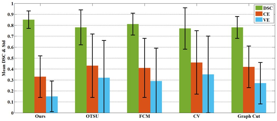
The mean and standard deviation of DSC, CE and VE on the 36 testing samples by the proposed method and the other four traditinal methods using PET only.

Table. 2.

The mean and standard deviation (std) of DSC, CE and VE of the proposed co-segmentation method and traditional methods on PET

Method	DSC	CE	VE
Ours	0.85(0.08)	0.33(0.19)	0.15(0.14)
OTSU	0.78(0.16)	0.43(0.29)	0.32(0.34)
FCM	0.81(0.10)	0.41(0.27)	0.29(0.30)
CV	0.77(0.19)	0.46(0.29)	0.35(0.35)
Graph Cut	0.78(0.10)	0.42(0.19)	0.27(0.19)

A more intuitive visual comparison for three patients are shown in Fig. 13. As we can see, the boundaries of the segmentation results of the traditional methods on PET only were barely accurate (see Figs. 13(b)–(e), (g)–(h) and (l)–(o)). A main reason is that the tumor boundaries in PET are blurry due to the low spatial resolution in PET imaging. Moreover, traditional methods on PET tended to be over-segmented, as shown in Figs. 13(b)–(e). For the proposed co-segmentation method, because it integrated the features of CT images which has a clear boundary, its segmentation results were closer to ground truth, as shown in Fig. 13(a), (f) and (k). The experimental results demonstrated the effectiveness of the proposed co-segmentation method.

Fig. 13.

Visual comparison of the segmentation results (blue contour) of different methods and the ground truth (pink contour) for three patients (each row shows results for one patient). The results on the first patient by: (a) The proposed co-segmentation, and (b)-(e) traditional methods using PET only (OTSU, FCM, CV and Graph Cut); the result on the second patient by: (f) the proposed method, and (g)-(j) traditional methods using PET only (OTSU, FCM, CV and Graph Cut), The result on the third patient by: (k) the proposed method, and (l)-(o) traditional methods using PET only (OTSU, FCM, CV and Graph Cut).

3.4.3. Comparison with variational co-segmentation methods

In this comparison, both variational co-segmentation methods were validated on the same remaining 36 samples. Note that the FVM_CO_2 method got two different tumor volumes corresponding to the PET image and the CT image respectively.

Quantitative evaluation indexes (DSC, CE and VE) for different methods in this comparison experiment are listed in Table 3. Fig. 14 shows their averages over all testing samples. As we can see, the FVM_CO_1 method (DSC=0.82) was superior to the other variational co-segmentation method FVM_CO_2 (DSC=0.80 on PET and DSC=0.73 on CT). The proposed method had a better performance (DSC=0.85). Fig. 15 shows the performance comparison for all 36 samples among the proposed method and two other variational co-segmentation methods. The flatter curve (see the green curve in Fig. 15) and the smallest variance value (see Table 3) demonstrated that the proposed method performed the best according to both accuracy and robustness.

Table. 3.

The mean and standard deviation (std) of DSC, CE and VE of the proposed method and all comparison methods.

Method	DSC	CE	VE
Ours	0.85(0.08)	0.33(0.19)	0.15(0.14)
FVM_CO_1	0.82(0.10)	0.39(0.25)	0.25(0.28)
FVM_CO_2 on PET	0.80(0.12)	0.42(0.26)	0.30(0.27)
FVM_CO_2 on CT	0.73(0.14)	0.61(0.33)	0.48(0.38)

Fig. 14.

The mean and standard deviation of DSC, CE and VE on the 36 testing samples due to the proposed method and the other two variatinal co-segmentation methods.

Fig. 15.

Performance comparison with the traditional co-segmentation methods. (a) DSC, and (b) VE, all on 36 testing samples. The proposed method (green) had a better performance and was more robust than both traditional co-segmentation methods. The FVM_CO_1 method and FVM_CO_2 method totally failed for several patients (e,g, patients 12, 13, 17, 27), while the proposed still had decent performance for these patients.

Fig. 16 shows three segmentation examples for the proposed method and the two variational co-segmentation methods. The proposed method performed better than the two variational co-segmentation methods. As shown in Figs. 16(b)–(d) and (j)–(l), over-segmentation happened because of the difference between PET and CT. for both FVM_CO_1 and FVM_CO_2. A possible reason for the failure of the two variational co-segmentation methods is that these two methods have no adaptive way of combining the advantages from the PET and CT. These methods failed to balance the influence between the two modalities. As shown in Figs. 16(b)–(d), some voxels in the tumor areas were not classified correctly, and the boundary between the tumor and the surrounding normal tissue was also not localized correctly, because of the high influence of the surrounding normal soft-tissue, which has the similar intensity as the tumor in the CT image (see Fig. 16(h)). Besides, voxels with a low intensity (the cold areas) in the PET image were classified as background owing to the high influence of the PET image for the variational co-segmentation, as shown in Figs. 16(j)–(l). In contrast, the segmentation results of the proposed method were more consistent with the ground truth, as shown in Fig. 16(a), (e) and (i).

Fig. 16.

Visual comparison of the segmentation results (blue contour) of different methods and the ground truth (pink contour) for three patients (each arrow shows results for one patient). The result on the first patient by: a) the proposed method, (b) FVM_CO_1, (c) FVM_CO_2 on PET, and (d) FVM_CO_2 on CT, respectively. The result on the second patient by: (e) the proposed method, (f) FVM_CO_1, (g) FVM_CO_2 on PET, and (h) FVM_CO_2 on CT, respectively. The result on the third patient by: (i) the proposed method, (j) FVM_CO_1, (k) FVM_CO_2 on PET, and (l) FVM_CO_2 on CT, respectively.

4. Discussion

In this paper, we proposed a novel multi-modality deep fully convolutional neural network for tumor co-segmentation in PET/CT. Our method can be also used as a general multi-modality co-segmentation framework of other imaging modalities. The proposed network realized feature fusion automatically by establishing two parallel branches for feature map extraction from two modalities and a fusion network for feature re-extraction. Experimental result demonstrated that the proposed co-segmentation network can combine the advantages of the two imaging modalities effectively.

In the last several years, with the development of deep learning, CNN-based methods achieved good performance in image segmentation tasks, but most CNN-based methods worked only on single imaging modality. In clinic, a tumor under different imaging modality may have very different appearance since different imaging modality describe tumor from different physical and biological aspects. These modalities provide complemental information to each other. Our study demonstrated that integrating different imaging modality is able to improve segmentation performance, and deep learning can be used for this purpose.

The proposed co-segmentation method makes full use of advantages from both PET and CT modalities: the high contrast in PET and the high spatial resolution in CT. On one hand, the high spatial resolution in CT helps to accurately localize tumor boundary in PET, in which the tumor boundary is typically blurry. On the other hand, the high contrast in PET helps to exclude the surrounding soft tissues from the segmentation result in CT, where the tumor and surrounding soft tissues often have the similar intensity. Besides, the proposed network was designed to be adaptive to the diversity of tumor size and shape, leading to a rapid training process. Moreover, the proposed network has a very fast prediction (segmentation) speed once the network was properly trained. It only spent 0.508s on average for each testing sample. Note that the parameters of the proposed network are fixed and do not need to be recalculated after training. In addition, the proposed network works in an end-to-end way without needing any cumbersome pre-processing and post-processing. With a high performance, the proposed automatic segmentation process might be useful in clinic where physicians typically spent lots of time to manually annotate the tumor for disease diagnosis and treatment planning.

We designed a network with cascaded convolutional blocks for feature fusion in this study. The feature fusion part automatically integrated information from PET and CT for tumor segmentation. [22, 28]. The weighting parameters of the loss functions w⁽¹⁾, w⁽²⁾, w^fusion (see Eq. (2)) were manually adjusted, which would affect the segmentation performance. In our study, these parameters were set to be 0.5, 0.5 and 1 respectively to have the optimal segmentation results. Furthermore, there are some directions should be considered for future research. Sometimes contradictory rather than complementary information between the two modalities caused conflicts in defining the boundaries of the tumor. A decision matrix, which determines the final result should believe which modality, will be needed. Besides, it would be interesting to see if there are better ways to re-extract features from PET/CT feature maps. It would be also interesting to see if the trained network can be transferred to other datasets without re-training. These will be our future work in this topic.

5. Conclusion

In this study, we proposed a novel multi-modality, full convolutional neural network for co-segmentation of tumor in PET-CT images. The proposed neural network is able to make full use of the advantages from both modalities (the metabolic information from PET and anatomical information from CT). The proposed neural network was validated on a clinic PET/CT dataset of 84 patients with lung cancer. The results showed that the proposed network is effective, fast and robust and achieved significant performance improvement over the other CNN-based method, traditional methods using PET or CT only, and two vairational co-segmentation methods.

References

- [1].Lecun Y, Bengio Y, Hinton G, Deep learning, Nature, 521 (2015) 436–444. [DOI] [PubMed] [Google Scholar]
- [2].Krizhevsky A, Sutskever I, Hinton GE, ImageNet classification with deep convolutional neural networks, in: International Conference on Neural Information Processing Systems, 2012, pp. 1097–1105. [Google Scholar]
- [3].Simonyan K, Zisserman A, Very deep convolutional networks for large-scale image recognition, arXiv preprint arXiv:1409.1556, (2014). [Google Scholar]
- [4].Szegedy C, Liu W, Jia Y, Sermanet P, Reed S, Anguelov D, Erhan D, Vanhoucke V, Rabinovich A, Going deeper with convolutions, in: Computer Vision and Pattern Recognition, 2015, pp. 1–9. [Google Scholar]
- [5].Gao XW, Hui R, Tian Z, Classification of CT brain images based on deep learning networks, Computer Methods & Programs in Biomedicine, 138 (2017) 49–56. [DOI] [PubMed] [Google Scholar]
- [6].Girshick R, Fast r-cnn, in: Proceedings of the IEEE international conference on computer vision, 2015, pp. 1440–1448. [Google Scholar]
- [7].Girshick R, Donahue J, Darrell T, Malik J, Rich Feature Hierarchies for Accurate Object Detection and Semantic Segmentation, in: Proceedings of the IEEE international conference on computer vision, 2014, pp. 580–587. [Google Scholar]
- [8].Redmon J, Divvala S, Girshick R, Farhadi A, You Only Look Once: Unified, Real-Time Object Detection, in: Proceedings of the IEEE international conference on computer vision, 2016, pp. 779–788. [Google Scholar]
- [9].Ren S, He K, Girshick R, Sun J, Faster R-CNN: Towards Real-Time Object Detection with Region Proposal Networks, IEEE Transactions on Pattern Analysis & Machine Intelligence, 39 (2017) 1137–1149. [DOI] [PubMed] [Google Scholar]
- [10].Graves A, Jaitly N, Towards end-to-end speech recognition with recurrent neural networks, in: International Conference on Machine Learning, 2014, pp. 1764–1772. [Google Scholar]
- [11].Sutskever I, Vinyals O, Le QV, Sequence to sequence learning with neural networks, Advances in neural information processing systems, 2 (2014) 3104–3112. [Google Scholar]
- [12].Long J, Shelhamer E, Darrell T, Fully convolutional networks for semantic segmentation, in: Computer Vision and Pattern Recognition, 2015, pp. 3431–3440. [DOI] [PubMed] [Google Scholar]
- [13].Badrinarayanan V, Kendall A, Cipolla R, SegNet: A Deep Convolutional Encoder-Decoder Architecture for Scene Segmentation, IEEE Transactions on Pattern Analysis & Machine Intelligence, 39 (2017) 2481–2495. [DOI] [PubMed] [Google Scholar]
- [14].Chen LC, Papandreou G, Kokkinos I, Murphy K, Yuille AL, Semantic Image Segmentation with Deep Convolutional Nets and Fully Connected CRFs, Computer Science, (2014) 357–361. [DOI] [PubMed] [Google Scholar]
- [15].Chen L-C, Papandreou G, Kokkinos I, Murphy K, Yuille AL, Deeplab: Semantic image segmentation with deep convolutional nets, atrous convolution, and fully connected crfs, arXiv preprint arXiv:1606.00915, (2016). [DOI] [PubMed] [Google Scholar]
- [16].Chen L-C, Papandreou G, Schroff F, Adam H, Rethinking atrous convolution for semantic image segmentation, arXiv preprint arXiv:1706.05587, (2017). [Google Scholar]
- [17].Ronneberger O, Fischer P, Brox T, U-Net: Convolutional Networks for Biomedical Image Segmentation, in: International Conference on Medical Image Computing and Computer-Assisted Intervention, 2015, pp. 234–241. [Google Scholar]
- [18].Milletari F, Navab N, Ahmadi SA, V-Net: Fully Convolutional Neural Networks for Volumetric Medical Image Segmentation, in: Fourth International Conference on 3d Vision, 2016, pp. 565–571. [Google Scholar]
- [19].Shen H, Wang R, Zhang J, McKenna SJ, Boundary-Aware Fully Convolutional Network for Brain Tumor Segmentation, in: International Conference on Medical Image Computing and Computer-Assisted Intervention, Springer, 2017, pp. 433–441. [Google Scholar]
- [20].Goodfellow IJ, Pouget-Abadie J, Mirza M, Xu B, Warde-Farley D, Ozair S, Courville A, Bengio Y, Generative adversarial nets, in: International Conference on Neural Information Processing Systems, 2014, pp. 2672–2680. [Google Scholar]
- [21].Christ PF, Ettlinger F, Grün F, Elshaera MEA, Lipkova J, Schlecht S, Ahmaddy F, Tatavarty S, Bickel M, Bilic P, Automatic Liver and Tumor Segmentation of CT and MRI Volumes using Cascaded Fully Convolutional Neural Networks, arXiv preprint arXiv:1702.05970, (2017). [Google Scholar]
- [22].Song Q, Bai J, Han D, Bhatia S, Sun W, Rockey W, Bayouth JE, Buatti JM, Wu X, Optimal co-segmentation of tumor in PET-CT images with context information, IEEE Transactions on Medical Imaging, 32 (2013) 1685–1697. [DOI] [PMC free article] [PubMed] [Google Scholar]
- [23].Nigam I, Vatsa M, Singh R, Ocular biometrics: A survey of modalities and fusion approaches, Information Fusion, 26 (2015) 1–35. [Google Scholar]
- [24].Bagci U, Udupa JK, Yao J, Mollura DJ, Co-segmentation of Functional and Anatomical Images, Medical Image Computing and Computer-Assisted Intervention, 7512 (2012) 459–467. [DOI] [PMC free article] [PubMed] [Google Scholar]
- [25].Wang X, Ballangan C, Cui H, Fulham M, Eberl S, Yin Y, Feng D, Lung Tumor Delineation Based on Novel Tumor-Background Likelihood Models in PET-CT Images, IEEE Transactions on Nuclear Science, 61 (2014) 218–224. [Google Scholar]
- [26].Grady L, Random walks for image segmentation, IEEE Transactions on Pattern Analysis & Machine Intelligence, 28 (2006) 1768–1783. [DOI] [PubMed] [Google Scholar]
- [27].Boykov Y, Funkalea G, Graph Cuts and Efficient N-D Image Segmentation, International Journal of Computer Vision, 70 (2006) 109–131. [Google Scholar]
- [28].Ju W, Xiang D, Zhang B, Wang L, Kopriva I, Chen X, Random Walk and Graph Cut for Co-Segmentation of Lung Tumor on PET-CT Images, IEEE Transactions on Image Processing A Publication of the IEEE Signal Processing Society, 24 (2015) 5854–5867. [DOI] [PubMed] [Google Scholar]
- [29].Yu K, Chen X, Shi F, Zhu W, Zhang B, Xiang D, A novel 3D graph cut based co-segmentation of lung tumor on PET-CT images with Gaussian mixture models, in: SPIE Medical Imaging, 2016, pp. 97842V. [Google Scholar]
- [30].I.G.a.Y.B.a.A. Courville, Deep Learning, MIT Press, 2016. [Google Scholar]
- [31].Springenberg JT, Dosovitskiy A, Brox T, Riedmiller M, Striving for simplicity: The all convolutional net, arXiv preprint arXiv:1412.6806, (2014). [Google Scholar]
- [32].Glorot X, Bordes A, Bengio Y, Glorot X, Bordes A, Bengio Y, Deep Sparse Rectifier Neural Networks, in: International Conference on Artificial Intelligence and Statistics, 2012, pp. 315–323. [Google Scholar]
- [33].Srivastava N, Hinton G, Krizhevsky A, Sutskever I, Salakhutdinov R, Dropout: a simple way to prevent neural networks from overfitting, Journal of Machine Learning Research, 15 (2014) 1929–1958. [Google Scholar]
- [34].Kingma D, Ba J, Adam: A method for stochastic optimization, arXiv preprint arXiv:1412.6980, (2014). [Google Scholar]
- [35].Chuang KS, Tzeng HL, Chen S, Wu J, Chen TJ, Fuzzy c-means clustering with spatial information for image segmentation, Computerized Medical Imaging & Graphics the Official Journal of the Computerized Medical Imaging Society, 30 (2006) 9–15. [DOI] [PubMed] [Google Scholar]
- [36].Chan TF, Vese LA, Active Contour Without Edges, IEEE Transactions on Image Processing, 10 (2001) 266–277. [DOI] [PubMed] [Google Scholar]
- [37].Pratondo A, Chui C-K, Ong S-H, Integrating machine learning with region-based active contour models in medical image segmentation, Journal of Visual Communication and Image Representation, 43 (2017) 1–9. [Google Scholar]
- [38].Gong M, Tian D, Su L, Jiao L, An efficient bi-convex fuzzy variational image segmentation method, Information Sciences, 293 (2015) 351–369. [Google Scholar]
- [39].Tan S, Li L, Choi W, Kang MK, D’Souza WD, Lu W, Adaptive region-growing with maximum curvature strategy for tumor segmentation in (18)F-FDG PET, Physics in Medicine & Biology, 62 (2017) 5383–5402. [DOI] [PMC free article] [PubMed] [Google Scholar]
- [40].Li L, Wang J, Lu W, Tan S, Simultaneous tumor segmentation, image restoration, and blur kernel estimation in PET using multiple regularizations, Computer Vision & Image Understanding, 155 (2017) 173–194. [DOI] [PMC free article] [PubMed] [Google Scholar]
- [41].Dewalle-Vignion AS, Betrouni N, Lopes R, Huglo D, Stute S, Vermandel M, A new method for volume segmentation of PET images, based on possibility theory, IEEE Transactions on Medical Imaging, 30 (2011) 409–423. [DOI] [PubMed] [Google Scholar]
- [42].Hatt M, Rest CCL, Turzo A, Roux C, Visvikis D, A Fuzzy Locally Adaptive Bayesian Segmentation Approach for Volume Determination in PET, IEEE Transactions on Medical Imaging, 28 (2009) 881–893. [DOI] [PMC free article] [PubMed] [Google Scholar]