Atmospheric heat and moisture transport to energy‐ and water‐limited ecosystems

Abstract

The land biosphere is a crucial component of the Earth system that interacts with the atmosphere in a complex manner through manifold feedback processes. These relationships are bidirectional, as climate affects our terrestrial ecosystems, which, in turn, influence climate. Great progress has been made in understanding the local interactions between the terrestrial biosphere and climate, but influences from remote regions through energy and water influxes to downwind ecosystems remain less explored. Using a Lagrangian trajectory model driven by atmospheric reanalysis data, we show how heat and moisture advection affect gross carbon production at interannual scales and in different ecoregions across the globe. For water‐limited regions, results show a detrimental effect on ecosystem productivity during periods of enhanced heat and reduced moisture advection. These periods are typically associated with winds that disproportionately come from continental source regions, as well as positive sensible heat flux and negative latent heat flux anomalies in those upwind locations. Our results underline the vulnerability of ecosystems to the occurrence of upwind climatic extremes and highlight the importance of the latter for the spatiotemporal propagation of ecosystem disturbances.

Using a Lagrangian trajectory model driven by atmospheric reanalysis data, we show how heat and moisture advection affect gross carbon production at interannual scales and in different ecoregions across the globe. Our results underline the vulnerability of ecosystems to the occurrence of upwind climatic extremes and highlight the importance of the latter for the spatiotemporal propagation of ecosystem disturbances.

Introduction

Terrestrial ecosystems sequester large quantities of carbon via photosynthesis: soil and vegetation store roughly triple the amount of carbon compared with the atmosphere. The land biosphere has absorbed about a quarter of all anthropogenic carbon dioxide (CO₂) emissions since the Industrial Revolution ¹ and, together with the ocean, dominates natural carbon removal processes at decadal timescales. ² Therefore, terrestrial biomes bear significant potential to dampen the impact of rising greenhouse gas concentrations. ³ The CO₂ fixed by plants and converted to organic carbon in ecosystems is collectively referred to as gross primary production (GPP), which is partly counteracted by the release of CO₂ through autotrophic respiration; their balance determines biomass growth, thus the net carbon sink by vegetation. At the ecosystem scale, heterotrophic respiration by soil microbes and animals, ⁴ but also disturbances—such as wildfires, ⁵ storms and gale winds, ⁶ , ⁷ landslides, ⁸ beetles, ⁹ , ¹⁰ or logging ¹¹ —reduce the net carbon sink. Globally, increasing GPP trends have been observed in recent decades following the enhanced CO₂ concentrations ¹² and despite potential nutrient constraints. ¹³ , ¹⁴

Terrestrial ecosystems also affect weather and climate through transpiration, induced changes in winds and mesoscale circulation, ¹⁵ , ¹⁶ and impacts on the surface radiation budget associated with the low albedo of vegetation. ¹⁷ , ¹⁸ Plants need water, light, and nutrients to survive, and thus their productivity depends on the properties of the soil in which they grow and the climate conditions they are exposed to. In the long term, the average patterns of precipitation, temperature, and solar radiation determine the dominant natural ecosystem in a region, ¹⁹ which enables a categorization of ecosystems into water and energy limited. ²⁰ At interannual scales, climate variability dictates the dynamics in vegetation productivity. ²¹ Whether the terrestrial carbon sink is primarily driven by precipitation or temperature at interannual scales remains highly controversial to this day. ²² , ²³

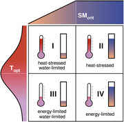
As illustrated in Figure 1, air temperatures are generally below the respective optimum in energy‐limited ecosystems, ²⁴ hence periods of anomalously high temperatures tend to enhance GPP. ²⁵ By contrast, soil moisture is often below the critical level in water‐limited regions, thus plant productivity is hampered when precipitation becomes even lower. ²⁶ , ²⁷ Moreover, in climate regimes that are both dry and hot, ecosystems are often not only water limited but also subject to heat stress: temperature increases may be detrimental to GPP. ²⁴ Given the negative effects of water and heat stress on productivity, the projected aggravation of droughts and heatwaves may reduce the terrestrial ecosystem carbon sink. ²⁸ During the last decades, heatwave and drought events caused a net loss of carbon from the terrestrial biosphere, ²⁹ thus supporting this expectation. For example, the 2003 mega‐heatwave in Western Europe resulted in a multiple years’ worth of net carbon uptakes being undone. ³⁰ During the 2010 mega‐heatwave in European Russia, the combined effect of elevated temperatures, above‐average solar radiation, low relative humidity, and reduced precipitation increased GPP in northern forests, yet croplands and more southern forests suffered from a strong decrease in productivity. ³¹ Part of this was related to species‐dependent responses: isohydric species (e.g., Aleppo pine trees ³² ) close their stomata more efficiently to conserve water compared with anisohydric ones (e.g., most crops ³³ ). Other hydraulic traits—such as root depth, xylem conductivity, or water use efficiency—are also crucial in determining the impact of water and heat stress on productivity. ²⁷ , ³⁴

Figure 1.

Ecosystems’ optimum temperature ²⁴ and a minimum (critical) level of soil moisture ²⁶ for which productivity is maximized (T_opt and SM_crit, respectively). As soon as T_opt is exceeded, heat advection is expected to have adverse effects on productivity (heat‐stressed types, I and II), whereas higher heat advection is favorable below T_opt (energy‐limited types, III and IV). Similarly, if soils are below SM_crit, productivity is reduced (water‐limited types, I and III). Note that this schematic is a simplification: it does not account for adverse effects of waterlogging on productivity; ⁹⁰ it illustrates the temperature optimality function as symmetric, and it depicts the soil moisture function as piecewise linear.

While the importance of local climate for vegetation dynamics has been well established, the larger‐scale mechanisms responsible for these local climatic conditions remain largely unexplored in the context of terrestrial ecosystem functioning. As the atmosphere transports heat and moisture through continuous circulation, ³⁵ local climate is ultimately determined not just by the surface–atmosphere heat and moisture fluxes, in conjunction with the entrainment at the top of the atmospheric boundary layer (ABL) from aloft, but also by the heat and moisture advected from upwind regions. The importance of moisture advection is illustrated by the vast amounts of water evaporating over the oceans that result in continental precipitation, often thousands of kilometers downwind. ³⁶ The relevance of atmospheric moisture transport for the occurrence of extreme precipitation ³⁷ , ³⁸ , ³⁹ and drought events ⁴⁰ , ⁴¹ , ⁴² , ⁴³ has been extensively studied. In addition, analyses of atmospheric heat advection have enabled new insights into the occurrence of heatwaves ⁴⁴ , ⁴⁵ and the propagation of drought and heatwaves as compound events. ⁴⁶ , ⁴⁷ On the other hand, the dependency of terrestrial ecosystem dynamics on moisture advection has seldom been investigated, ⁴² , ⁴⁸ and, to the authors’ knowledge, no emphasis has been placed on the role of heat advection for primary productivity. ²⁹

Here, we make the use of a recently introduced Lagrangian framework driven by reanalysis data (see below) to trace the origins of heat and moisture in water‐ and energy‐limited ecosystems worldwide and to test two hypotheses. The first is that the atmospheric inflow of moisture and heat critically influences ecosystem productivity and thus may be utilized for the estimation of GPP. To test this hypothesis, the links between growing‐season GPP and concurrent atmospheric transport of moisture and heat are explored, focusing on two ecoregions in Europe, one primarily water limited and one primarily energy limited. The second hypothesis is that growing seasons with unusually low peak productivity in water‐limited ecosystems are associated with (positive) negative anomalies in (heat) moisture advection. To test this, the focus is shifted toward five semiarid ecoregions located in different continents. Overall, this study aims to improve the understanding of the effect of heat and moisture advection on ecosystem productivity worldwide.

Data and methods

In this study, a Lagrangian trajectory model was employed to identify the origins of advected heat and moisture, including a bias correction based on observations. To investigate the first hypothesis, the analysis begins with two European ecoregions, followed by an extension to five global ecoregions for the second hypothesis. In the following sections, data and methods are separately presented.

Data

Global GPP data from FLUXCOM RS+METEO, ⁴⁹ , ⁵⁰ available at a horizontal resolution of 0.5 × 0.5° and from 1980 to 2013, were used. This dataset, based on eddy‐covariance and satellite observations, was employed at monthly timescales and downscaled to 0.25 × 0.25° via bilinear interpolation to analyze the effect of local climate variables on GPP in Europe, and then upscaled to 1.0 × 1.0° to define global ecoregions. To avoid the influence of long‐term trends in GPP, ⁵¹ all time series were calculated on the basis of the native resolution and area weighted before being linearly detrended.

Data from the European Centre for Medium‐Range Weather Forecasts (ECMWF) reanalysis (ERA‐Interim) ⁵² were employed to drive the Lagrangian trajectory model FLEXPART. Data include 3D wind, humidity, and temperature fields at 1.0 × 1.0° horizontal resolution and at 61 vertical levels (1000–0.1 hPa). The reader is referred to Ref. 53 for a detailed list of FLEXPART input variables.

In addition, precipitation data were taken from Multi‐Source Weighted‐Ensemble Precipitation (MSWEP) version 1.1, available from 1979 to 2015 at 3‐hourly steps and 0.25 × 0.25° resolution and obtained by merging gauge, satellite, and reanalysis data. ⁵⁴ Two‐meter air temperatures were obtained from CRUNCEP version 7, a blend of Climatic Research Unit data and National Centers for Environmental Prediction reanalysis data, available in 6‐hourly steps from 1901 to 2016 at 0.5 × 0.5° resolution. ⁵⁵ Data were downscaled to 0.25 × 0.25° via bilinear interpolation.

Surface sensible and latent heat (or evaporation) fluxes were taken from the Global Land Evaporation Amsterdam Model (GLEAM) version 3.2a. ⁵⁶ , ⁵⁷ GLEAM is a process‐based (yet semiempirical) model ingesting satellite and reanalysis data that is primarily intended to estimate terrestrial evaporation but from which sensible heat fluxes can be obtained as the residual in the surface energy balance. Data are available from 1980 to present, at daily timesteps and 0.25 × 0.25° resolution. Over oceans, Objectively Analyzed Air–Sea Heat Fluxes (OAFlux) data were employed. ⁵⁸ OAFlux data are publicly available at daily timesteps from 1985 until present, and at 1.0 × 1.0° resolution. Note that owing to the lack of daily OAFlux data before 1985, ocean surface sensible and latent heat fluxes were taken from ERA‐Interim from 1980 to 1985.

Methods

Ecoregion delineation

The first part of the study evaluates the impact of atmospheric advection on ecosystem productivity for two ecoregions in Europe, one water and one (predominantly) energy limited (see Fig. 2A). The second part of the study aims to unravel the impact of heat and moisture advection on the occurrence of low productivity extremes and focuses on five global ecoregions with large interannual variability in ecosystem productivity (see Fig. 2B). In both parts, these ecoregions are considered as sinks in the application of the Lagrangian heat and moisture tracking framework (see below). The first part of the study focuses on the growing season over Europe, here defined as February through April. Following the rationale that water and energy limitations can be defined on the basis of the relationship between GPP and local climatic variables, growing‐season GPP was correlated with the corresponding air temperature (CRUNCEP) and precipitation (MSWEP), per pixel, and at a resolution of 0.25 × 0.25°. The resulting Spearman correlation coefficients were used to select a predominantly water‐limited and a predominantly energy‐limited ecoregion (Fig. 2A).

Figure 2.

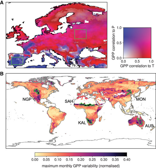
Delineation of the ecoregions considered as sinks of heat and moisture. (A) Spearman correlation coefficients between growing‐season (FMA) GPP and local temperature (strong relationships indicated by red), and between GPP and precipitation (blue), based on 1980–2013. The two green boxes correspond to the (predominantly) water‐ and energy‐limited ecoregions, respectively, used in the first half of the study. (B) Global hotspots of interannual GPP variability, based on the maximum normalized monthly standard deviation of GPP (1980–2013). The green contours mark the five ecoregions subject to strong interannual GPP variability that are investigated in the second half of the study.

The second part of the study extends to the entire globe, focusing on ecoregions of high GPP interannual variability and potentially subject to strong interannual anomalies in heat and moisture advection. To define these ecoregions, the GPP data were first resampled to the same 1.0 × 1.0° grid employed for tracking heat and moisture (see below). Then, standard deviations per pixel were calculated for each month of the year, considering the 1980–2013 record (i.e., based on 34 values). The month of maximum interannual variability per pixel was then selected on the basis of these standard deviations. The standard deviation for that month, hereafter referred to as the “peak month,” was then normalized by the annual average GPP of the corresponding pixel. Regions in which this normalized standard deviation exceeds 0.25 and for which the timing of the peak month agrees within ±1 month were selected—this procedure is analogous to that in Ref. 48 and results in five ecoregions worldwide (Fig. 2B). Note that the peak month varies per ecoregions (Fig. S1, online only).

Lagrangian simulations

The heat and moisture tracking framework used here is based on the Lagrangian particle dispersion model FLEXPART v9.0, ⁵³ , ⁵⁹ which was originally developed to trace radioactive particles in the atmosphere but has already been applied in many studies of the hydrological cycle (e.g., Ref. 36, 37, and 60). FLEXPART represents the flowing atmosphere by many parcels of air that can be tracked back in time, and enables the identification of moisture and heat origins through parcel property changes along those backward trajectories (Ref. 47 and Keune et al., in preparation).

In this study, the European FLEXPART simulations from Ref. 47 and 61 and the global simulations from Ref. 62 were employed to address the two main hypotheses, respectively. In both simulations, FLEXPART was driven by the ERA‐Interim reanalyses and initialized with approximately 2 million homogeneously distributed parcels of identical mass. The different domain sizes (i.e., European versus global) represent the most notable difference between the simulations; consequently, the European setup has a higher parcel density and is thus associated with less noise. For details about the setup of both model simulations, the reader is referred to the above referenced studies. The model output comprises 6‐hourly values of parcel positions (latitude, longitude, and height) and properties (e.g., density, specific humidity, and temperature) and the respective ABL height, which enables a process‐based quantification of source–receptor relationships. ⁶³

Estimation and attribution of heat and moisture advection

The advection of heat and moisture was determined by a “backward analysis” in four steps: (1) selection of air parcels residing over ecoregions, (2) tracking of selected parcels back in time, (3) diagnosis of source regions, and (4) summing of uptakes across each trajectory. The first step differs between heat and moisture. To assess the origin of advected heat in the atmosphere, only air parcels arriving in the ABL of the respective ecoregion were analyzed, following the methodology described in Ref. 47. For moisture, only air parcels that ultimately result in precipitation over the corresponding ecoregion were selected, which thus led to different subsets of air parcels (for heat and moisture) that were subsequently traced back in time. In the second step, backward trajectories of those selected parcels were constructed. In reference to the global average residence time of moisture in the atmosphere ⁶⁴ and the inherent limits posed by trajectory inaccuracies, ⁶⁵ backward trajectories up to 10 days were evaluated—the relevance of this 10‐day threshold is explored further below. In the third step, changes of potential temperature and specific humidity, assumed to be associated with surface sensible and latent fluxes, were calculated; locations where temperature and humidity increase over time indicate heat and moisture source regions, respectively. As in Ref. 63, positive changes between 6‐hourly analysis steps (00, 06, 12, and 18 UTC), that is, heat and moisture “uptakes,” were allocated to intermediate parcel positions (at 03, 09, 15, and 21 UTC) and calculated as geographical midpoints. For simplicity, the advected surface sensible heat (H_adv) is referred to as “advected heat” hereafter, and the advected surface evaporation leading to precipitation (E_adv(P)) is referred to as “advected moisture.”

A series of process‐based criteria were applied during these four steps. The ABL is assumed to be well mixed: moisture increases within the ABL reflect surface evaporation events, and potential temperature increases reflect surface sensible heat fluxes, constituting the backbone of our moisture and heat tracking framework. Concerning heat, a similar approach has been applied by, for example, Ref. 44, in which the authors were able to disentangle temperature increases caused by adiabatic compression from diabatic heating because of surface sensible heating. Building upon their findings, we implemented a similar approach with which we can quantify the surface sensible heat flux from changes in potential temperature globally. To this end, the same ABL definition as in Ref. 47 was used to diagnose both sensible heat and evaporation, based on 6‐hourly changes in dry static energy (s) and specific humidity (q) along parcel trajectories. In short, the largest among the two ABL heights associated with potential uptakes (one at the beginning and one at the end of any 6‐hourly period) and at the corresponding parcel location serves as a maximum allowed height. Only air parcels that remain below this maximum height during s or q uptakes are considered. For precipitation, a relative humidity threshold of 80% was employed, as in Ref. 63. A minimum threshold of q change was considered for evaporation ($\mathrm{\Delta }{q}_{min(E)}=0.2\mathrm{g}/\mathrm{kg}$) and precipitation ($\mathrm{\Delta }{q}_{min(P)}=-0.2\mathrm{g}/\mathrm{kg}$). ⁶³ Analogously, a minimum s increase ($\mathrm{\Delta }{s}_{min(H)}=1\mathrm{kJ}/\mathrm{kg}$, corresponding to a potential temperature rise of 1 K) was required to diagnose a sensible heat uptake—see Ref. 47. Note that in this framework, $\mathrm{\Delta }s>\mathrm{\Delta }{s}_{min(H)}$ only accounts for the effect of surface heating on the ABL, not explicitly considering processes such as heat diffusion, radiation, and phase changes. Similarly, $\mathrm{\Delta }q>\mathrm{\Delta }{q}_{min(E)}$ within the ABL is assumed to represent surface evaporation.

It is important to note that even though our ABL definition is designed to avoid the detection of changes owing to air parcels being mixed into the ABL from aloft, entrainment of heat and (to a lesser extent) moisture still occurs. Higher surface sensible heat fluxes imply stronger ABL growth, and thus more entrainment of tropospheric air at higher potential temperature than the ABL (e.g., Ref. 66). Entrainment generally contributes about 20% of additional heat compared with surface heating under purely convective conditions. ⁶⁷ In the presence of high mechanical turbulence, this ratio has been reported to increase up to, or even beyond, 30–40%, ⁶⁸ , ⁶⁹ , ⁷⁰ being influenced by the vertical stability of the atmosphere, surface conditions, and boundary layer dynamics. ⁷¹ As a consequence, the approach used here tends to overestimate surface sensible heat fluxes and is thus accompanied by a bias correction (see further below).

Thresholds ($\mathrm{\Delta }{q}_{min(P)}$, $\mathrm{\Delta }{q}_{min(E)}$, and $\mathrm{\Delta }{s}_{min(H)}$) were applied to reduce errors associated with, for example, numerical noise, interpolation, or the incorporation of mixing processes. ⁷² To assess the influence of the choice of values for these thresholds, a sensitivity analysis was performed in the first part of the study for which $\mathrm{\Delta }{q}_{min(P)}$, $\mathrm{\Delta }{q}_{min(E)}$, and $\mathrm{\Delta }{s}_{min(H)}$ were either set to zero, or doubled. Moreover, the ABL criterion from Ref. 47 was (1) relaxed (i.e., air parcels are only required to reside within the maximum allowed height either before or after a potential uptake event), as well as (2) tightened (air parcels must be in the ABL both before and after an uptake, based on the respective ABL height, not the maximum). Next, moisture and heat uptakes were corrected (or “discounted”; see Ref. 63) by moisture losses (e.g., precipitation) or cooling (e.g., nighttime cooling) occurring en route to the sink region. For moisture, this procedure enables the representation of each q uptake (source) as a fraction of the total specific humidity before any precipitation event over the ecoregions (sink), and thus the estimation of source–sink relationships. As remote source regions are usually separated by several intermittent precipitation events from the ecoregion, these areas naturally contribute less precipitating moisture than source regions in close vicinity of the ecoregion. The applied discounting can thus effectively shorten trajectories, leading to atmospheric moisture residence times well below 10 days, in analogy with the results of Ref. 73 and 74. Although the resulting residence times might be on the lower end of the literature‐reported estimates (see references therein), the corrections en route are essential to achieve mass and energy conservation.

Even though the choice of a maximum trajectory length is a hard limit for the residence time, the latter is first and foremost a consequence of the frequency and magnitude of moisture uptakes and losses along trajectories. Therefore, the residence times are not explicitly prescribed here, but rather limited to a maximum of 10 days because of accuracy constraints. ⁶¹ , ⁶³ , ⁶⁵ , ⁷⁵ This choice can be considered as a trade‐off between precision and unallocated moisture owing to not tracking further back in time. Still, the ensemble of simulations was expanded here to explore the influence of 5‐ and 15‐day maximum trajectories. The final ensemble thus consists of 27 individual members. Note that, in this framework, heat is treated analogously to moisture. ⁴⁷ As already reported by Ref. 76 and confirmed by our analysis, despite regional differences, extending trajectories beyond 10 days only results in a slight increase in “explained moisture” (see Figs. S2 and S3, online only).

Finally, in the fourth step, the total advection of heat and moisture to an ecoregion was approximated by the sum of the uptakes of s and q through

$$\begin{array}{ccc}& & {\mathrm{H}}_{\mathrm{adv}}\approx \sum _{j=1}^{k_h}\sum _{t=0}^{-20,-40,-60}{(\mathrm{\Delta }s)}_{(j,t)}\times F_H,\hfill \\ & & {\mathit{F}}_H=1\mathrm{if}\mathrm{H}\mathrm{diagnosed},\mathrm{else}{\mathit{F}}_H=0,\hfill \end{array}$$ (1)

and

$$\begin{array}{ccc}& & {\mathrm{E}}_{\mathrm{adv}(\mathrm{P})}\approx \sum _{j=1}^{k_p}\sum _{t=0}^{-20,-40,-60}{(\mathrm{\Delta }q)}_{j,t}\times F_E,\hfill \\ & & {\mathit{F}}_E=1\mathrm{if}\mathrm{E}\mathrm{diagnosed},\mathrm{else}{\mathit{F}}_E=0,\hfill \end{array}$$ (2)

respectively. The sum was calculated over all k_h and k_p available trajectories and 40 timesteps t extending into the past by 6‐hourly increments for the trajectory length of 10 days (as well as 5 or 15 days in case of the aforementioned ensemble calculations). Note that only positive and discounted contributions are considered through the multiplication by F_H and F_E, which are 1 if the contributions are associated with surface sensible heat fluxes (H) and surface evaporation (E), and 0 otherwise. H_adv and E_adv(P) were calculated on the basis of backward trajectories for every 6‐hourly timestep, and daily sums of E and H were bias corrected with observation‐based evaporation and sensible heat datasets from GLEAM (regridded to 1.0 × 1.0°) and OAFlux, respectively (see above and Ref. 47 for details). Finally, the daily transport of heat and moisture from surrounding and remote source regions to each ecoregion was aggregated over time to obtain single values for H_adv and E_adv(P) per season, representing the average advection of heat and moisture.

Estimation of advection impacts on productivity

For the first part of the study, growing‐season GPP was related to the advection of heat and moisture to two primarily water‐ and energy‐limited ecoregions in Europe, for which only transport from beyond ecoregion boundaries was considered. To assess this relationship between GPP and advection, a multiple linear regression was employed and the variance of GPP explained by heat and moisture advection was expressed as the coefficient of determination. The linear regression was set up as:

$$GPP{}_{est}^{\prime }=aH{}_{adv}^{\prime }+bE{}_{adv\left(P\right)}^{\prime },$$ (3)

where the prime represents standardized anomalies with respect to the climatology, so that the intercept is zero, and the target variable is GPP′_obs. The resulting coefficient of determination was defined as:

$$R^2=SSR/SST,$$ (4)

where the regression sum of squares (SSR) was calculated as:

$$SSR=\sum _{j=1}^{J=34}{({\widehat{y}}_j-\overline{y})}^2,$$ (5)

that is, the squared differences between the predictor variable $\widehat{y}$, here anomalies of H_adv and E_adv(P), and the interannual mean of the target variable $\overline{y}$, here GPP′_obs, summed up over 34 seasons (1980–2013). Note that since the regression was based on standardized anomalies, $\overline{y}=\overline{G{P^{\prime }}_{est}}=0.$ Likewise, the total sum of squares (SST) was defined as:

$$SSR=\sum _{j=1}^{J=34}{(y_j-\overline{y})}^2.$$ (6)

For the second part of the study, area‐weighted ecoregion averages of GPP were calculated on the basis of the original GPP dataset at 0.5 × 0.5°, but only for the respective month of maximum interannual variability per pixel (i.e., the “peak month,” see Fig. S1, online only). The first and fourth quartiles—that is, the 9 years of lowest and highest GPP during the corresponding peak month—were considered separately. To take soil moisture memory into account, the heat and moisture advection during the peak month and the two antecedent months was considered. The advected heat and moisture during low GPP years was compared with the corresponding climatological expectation in order to focus on the anomalies in GPP and to assess their relationship to spatial anomalies in the origin and magnitude of moisture and heat advection.

Results and discussion

Estimation of ecosystem productivity based on moisture and heat advection

Considering that the local climate is inherently related to atmospheric advection, the first hypothesis—that vegetation dynamics thus also depend on heat and moisture advection—appears intuitive. To the authors’ knowledge, however, this relationship has never been scrutinized explicitly. Here, the influence of atmospheric advection of heat and moisture on ecosystem productivity was assessed by analyzing two ecoregions with differing characteristics: one water limited and one primarily energy limited (see Methods for the identification of these regions). Figure 2A shows the location of these two regions (in the Iberian Peninsula and Belarus), with the background illustrating the correlations of growing‐season GPP versus precipitation and temperature. The north–south gradients in these correlations, indicating a transition from energy‐ to water‐limited regimes, are in line with previous findings. ²⁰ , ⁷⁷ , ⁷⁸ , ⁷⁹ It is important to note, however, that these limitations may vary throughout the growing season; Mediterranean ecosystems, for example, are expected to slowly transition from being predominantly energy limited to water limited toward the end of the season (see, e.g., Ref. 80).

To assess the dependency of GPP on heat and moisture advection, and thus the potential to predict GPP on the basis of advection fluxes, a multiple linear regression model was used (see Methods). Figure 3 shows the time series of standardized anomalies of growing‐season productivity (GPP′_obs), advection anomalies (H′_adv and E′_adv(P)), the coefficients of determination (R ²) for both, and the estimated productivity (GPP′_est) for the two ecosystems. The results indicate that about half of the GPP′_obs variance can be attributed to atmospheric transport of heat and moisture for both ecosystems, with R ² = 0.48 for the ecoregion centered on Belarus and 0.62 for the Mediterranean ecoregion. For the latter (predominantly) water‐limited ecoregion, this is largely due to moisture advection, which by itself can already account for more than half of the variance of GPP′_obs (R ² = 0.56, blue bar in Fig. 3A). For the more energy‐limited ecoregion, the pattern is reversed, with moisture advection accounting for a lower share of GPP′_obs variance (R ² = 0.23, blue bar in Fig. 3B) than heat advection (R ² = 0.48).

Figure 3.

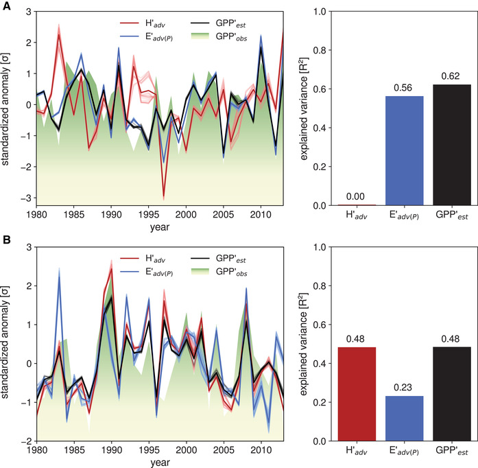
Standardized anomalies in heat (H′_adv) and moisture advection (E′_adv(P)) and growing‐season GPP (GPP′_obs). Individual members and ensemble mean are shown as semitransparent and opaque lines, respectively. The red and blue bars to the right of the time series denote the ensemble mean–explained variances of GPP′_obs by H′_adv and E′_adv(P), respectively, whereas the black bar denotes the estimated GPP anomaly (GPP′_est) obtained using the advection estimates of heat and moisture. Results are shown for (A) a predominantly water‐limited ecoregion over the Iberian Peninsula, and (B) a more energy‐limited region centered on Belarus. See Fig. 2A for the precise location of these two regions. Note that the red and blue bars do not add up to the black bar because of covariances between advected quantities (see Methods).

These findings are in line with expectations: the predominantly water‐driven ecoregion is affected mainly by advected moisture, whereas for the primarily energy‐limited ecoregion, heat advection is a more influential driver of GPP. Our hypothesis builds upon the knowledge that ecosystems respond to local climate conditions and that the latter, in turn, depend on advected heat and moisture fluxes. Therefore, the variance in GPP must also be explained by ecoregion′s local precipitation and temperature (see Fig. S4, online only). Moreover, it should be considered that not just heat advection but also radiation and local land feedbacks affect local temperatures. This explains the higher predictive power for local temperature (R ² = 0.71) than advected heat (R ² = 0.48) in the energy‐limited ecoregion. Advected moisture, however, shows a predictive power (R ² = 0.56) that is comparable to that of local precipitation (R ² = 0.48) in the water‐limited region.

It should be noted here that these results are subject to the uncertainty associated with assumptions in the Lagrangian heat and moisture tracking framework. To investigate this uncertainty, the default uptake thresholds were doubled and set to zero, the ABL criterion was relaxed and tightened, and the maximum trajectory length was lowered and increased by 5 days (see Methods for more details). As evident in Figure 3, each of the 27 individual advected heat and moisture estimates from the uncertainty ensemble results in similar GPP′_est (semitransparent black lines). The results of the Belarusian ecoregion (Fig. 3B) demonstrate low sensitivity to inherent assumptions: the R ² of moisture (heat) advection ranges from 0.22 to 0.25 (0.44–0.52), and thus varies between 0.44 and 0.52 for GPP′_est. For the primarily water‐limited ecoregion (Fig. 3A), the results are even more certain, as advected heat does not covary with GPP′_obs (R ² ranges from 0.0 to 0.01), whereas for advected moisture, R ² varies from 0.56 to 0.57, and from 0.61 to 0.63 for GPP′_est using both advection terms. In light of this uncertainty analysis, the results in Figure 3 indicate that ecosystem GPP can be deduced on the basis of moisture and heat advection during the growing season. The added value of studying atmospheric transfer of heat and moisture, instead of focusing on local climate variables as predictors of GPP variability, stems from the fact that advected quantities represent actual fluxes of energy and water and their origins can be inferred, so that GPP variability may be mechanistically connected to remote anomalies (e.g., sea surface temperature or soil moisture). These mechanisms could be exploited to allow for an earlier prediction of the ecosystem productivity.

Impact of advection on ecosystem productivity extremes

Since the influence of heat and moisture advection on ecosystem GPP has been demonstrated, next, we investigated whether low productivity growing seasons are associated with anomalous atmospheric inflow of heat and moisture. To address this question, five ecoregions around the globe with particularly high interannual variability in GPP were first identified using the maximum normalized standard deviation of GPP per month (Fig. 2B). The GPP variability from year to year is the largest during the respective hemispheric summer (Fig. S1, online only). The five ecoregions selected to test the aforementioned hypothesis include the Northern Great Plains (NGP) in North America, the Sahel (SAH), Western Manchuria and Eastern Mongolia (including parts of the Gobi Desert) (MON), continental Eastern Australia (AUS), and the Kalahari Desert (KAL). These ecoregions of strong GPP interannual variability correspond well to primarily transitional, water‐limited ecoregions ⁴⁸ , ⁸¹ that are prone to experience summer drought and heatwaves (type I regions in Fig. 1).

For all five ecoregions, Figure 4 shows the anomalies in the origin of advected heat and moisture (and their magnitude) during low‐GPP years (see Methods); the corresponding climatological source region is illustrated by black contours. Red (blue) colors in Figure 4A show areas that contribute more (less) heat during low‐GPP years than in average years. Analogously, green (brown) colors in Figure 4B indicate areas that contribute more (less) moisture. In general, Figure 4 shows that low‐GPP years are associated with positive anomalies of heat advection to the ecoregions and negative anomalies of moisture advection. Over NGP, low‐GPP years are associated with anomalously high amounts of heat originating in the west (Pacific coast of North America) and anomalously low contributions from the east. Simultaneously, most areas in North America contribute less moisture during these years. For SAH, the climatological moisture source (see black contour in Fig. 4B) consists mostly of the wetter savannah and forests in the south and the Gulf of Guinea (see also Ref. 82 and 83). However, the climatological heat source in SAH (see black contour in Fig. 4A) only partly overlaps with the moisture source, being located more toward the northeast. During low‐GPP years, SAH receives much more heat from the Sahara and much less moisture from more densely vegetated land areas in West Africa, the Gulf of Guinea, and the Atlantic Ocean. Similarly, low productivity times in AUS are associated with unusually large amounts of heat from inland and less moisture from the Pacific Ocean and the subtropical forests up north. Finally, both MON and KAL further confirm the hypothesis that anomalously high heat advection along with anomalously low moisture advection is associated with low GPP in these (type I) regions. Once again, it is mostly the continental heat and moisture sources in these regions that are responsible for the anomalies in GPP, and not the oceanic counterparts. This finding highlights the important role of upwind land–atmosphere interactions for downwind advection, temperature, precipitation, and ecosystem health. ⁴⁷ , ⁴⁸

Figure 4.

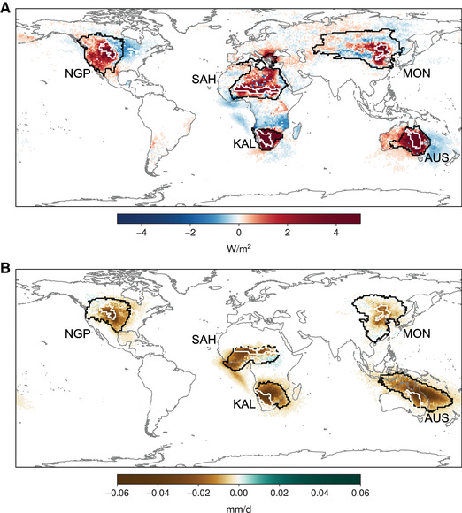
Anomalies in heat and moisture contributions during low‐GPP years. (A) Advected heat to our five ecoregions (white contours), expressed as anomalies for the respective peak month (Fig. 2B and Fig. S1, online only) and the two antecedent months. The climatological mean source regions are delineated using black contours, such that 80% of the average advected heat is accounted for by the smallest possible selection of source pixels. (B) Like panel A, but for advected moisture.

To facilitate the interpretation of the advection anomalies (Fig. 4), we explored the mean near‐surface wind direction and speed during low‐GPP years (Fig. 5A), as well as the sign of the wind speed anomalies (indicated by the color of each arrow)—wind direction anomalies are not shown because average wind directions are only marginally different (Fig. S5, online only). In addition, surface sensible heat (Fig. 5B), evaporation (Fig. 5C), and precipitation (Fig. 5D) anomalies are also illustrated. The average precipitation (accumulated during the month of low GPP and the two previous ones) falls below the climatological expectation for every single ecoregion (brown colors in Fig. 5D), in agreement with the moisture advection anomalies shown in Figure 4B. Note that the precipitation patterns seen in Figure 5D are induced by a mixture of anomalous circulation, anomalies in upwind turbulent fluxes, and the overall stability of the atmosphere. Upwind of NGP, sensible (latent) heat fluxes are higher (lower) than usual at low productivity times (see red and brown colors in Fig. 5B and C). NGP normally receives large amounts of moisture from the Gulf of Mexico via a low‐level jet. ⁸⁴ As evidenced by the anomalies in near‐surface winds, this mechanism is less efficient during low GPP years—see purple arrows between NGP and the Gulf of Mexico in Figure 5A, which indicate that less air is transported northward and more air is advected from the west and northwest, where the sensible heat flux (evaporation) is anomalously high (low).

Figure 5.

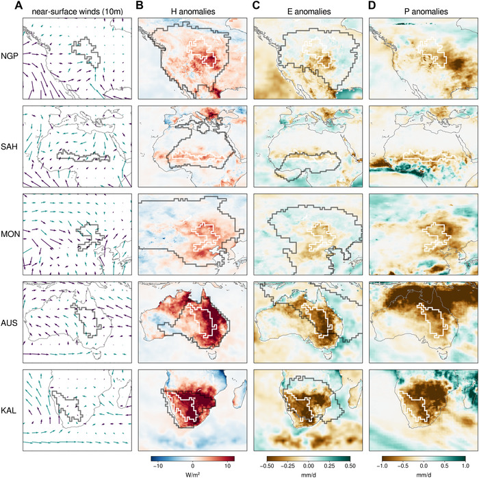
Winds and surface fluxes during low‐GPP years. (A) Mean near‐surface winds (ERA‐Interim) during low‐GPP seasons, colored green (purple) when mean wind speeds are higher (lower) than the climatology. (B) Surface sensible heat flux anomalies. (C) Evaporation anomalies. (D) Precipitation anomalies. In all plots, ecoregions are indicated by dark (A) or white (B–D) contours; for panels B and C, climatologically advected heat and moisture source regions are visualized by dark contours (as in Fig. 4), defined so that 80% of the average advected heat or moisture is explained by the lowest possible number of source pixels. Oceanic surface fluxes were bilinearly interpolated to match the native 0.25 × 0.25° horizontal resolution of terrestrial data used here.

Over SAH, anomalous amounts of sensible heat originate in the ecoregion itself during low‐GPP years, accompanied by above‐average transport of heat from the Sahara and even remote regions such as the (eastern) Mediterranean (Fig. 5A). The lower‐than‐usual wind speeds from the southwest (Fig. 5A) agree with the moisture uptake deficits in those regions (Fig. 4B) and may be connected to below‐average monsoonal circulation or a weak West African westerly jet. ⁸⁵ This leads to an enhanced Saharan influence and a reduced oceanic influence on SAH, and diminishes vegetation productivity. Inside and around MON, with the exception of the areas to the north, surface sensible heat is positively anomalous and evaporation negatively anomalous during low‐GPP years (Fig. 5B and C), and a large encompassing area tends to receive less precipitation than on average (Fig. 5D). Counterintuitively, both the inflow of air (Fig. 5A) and evaporation (Fig. 5C) in the northwest are anomalously high; yet, only a small area (green patch northwest of MON) actually contributes more moisture than usual to the precipitation in the region (Fig. 4B). As for SAH, (summer) precipitation in MON is largely controlled by the strength of the monsoon. ⁸⁶ , ⁸⁷ The extensive negative anomalies of advected moisture (Fig. 5B) that result in anomalies in precipitation (Fig. 5D) may thus be linked to the East Asian monsoon, for which breaks in the rainy period over MON are common. ⁸⁸ Moreover, the enhanced heat inflow from the west during low‐GPP years is arguably enabled by above‐average surface heating and not purely caused by anomalous circulation, as westerly inflow is not strengthened compared with normal years (Fig. 5A).

The two remaining ecoregions—AUS and KAL—are in the Southern Hemisphere, with February being their month of maximum GPP variability. KAL typically receives moisture from the Indian Ocean (black contour in Fig. 4B) via the Botswana low‐level jet, ⁸⁵ , ⁸⁹ but the source region also covers the northern forested regions. AUS, on the other hand, is adjacent to northern areas that receive almost exclusively monsoonal precipitation during austral summer. ⁸⁵ The analysis of wind patterns in Figure 5A confirms the results in Figure 4B: the Australian monsoon fuels moisture from the northwest, but the northern tropical forests also contribute to precipitation. During low‐GPP years, less air from the ocean arrives in the ecoregion (Fig. 5A, purple arrows to the north and east) and more comes from inland sources (Fig. 5A, green arrows to the (south)‐west); this, together with the strong sensible heat flux anomalies inland (Fig. 5B), explains the anomalously positive contribution of heat advection from continental areas shown in Figure 5A. Similarly, heat advection to KAL is enhanced during low‐GPP years and, as can be seen in the wind maps in Figure 5A, this is again not merely a consequence of unusual circulation but also related to anomalies in sensible heat fluxes (Fig. 5B). In fact, this analysis indicates that the anomalously high land sensible heat fluxes (Fig. 5B) extending far beyond the ecoregion itself in the upwind direction (Fig. 5A) are largely responsible for the heat advection anomalies downwind (Fig. 4A). This agrees with the findings by Ref. 47 for dry and hot events during European summers.

In summary, a common pattern emerges from these results: low productivity is associated with overall reduced moisture advection and enhanced heat transport. This highlights the fact that all these ecoregions that experience the highest interannual variability in productivity belong to type I in Figure 1. Furthermore, during low‐GPP years, there is a shift away from oceanic and toward continental source regions, which is most evident in ecoregions such as SAH and NGP. Particularly for AUS and KAL, the crucial contribution of upwind land–atmosphere feedbacks (Fig. 5B) to increased heat advection (Fig. 4A) is apparent: enabled by drought conditions upwind, the shift in remote land surface energy partitioning—away from latent and toward sensible heat fluxes—can strongly amplify advected heat and simultaneously diminish advected moisture. ⁴⁶ , ⁴⁷ Finally, even though the discussion has focused on the role of atmospheric advection when ecosystem productivity is below average, consistent findings are derived from the evaluation of high‐GPP years (Fig. S6, online only). As expected, the patterns in those years are reversed, as highly productive seasons are associated with below‐average heat advection and enhanced moisture transport in these ecoregions. Therefore, the Lagrangian analysis presented here demonstrates that anomalies in the atmospheric advection of heat and moisture in transitional climate regimes trigger extremes in ecosystem productivity.

Conclusion

To date, the role of combined atmospheric advection of heat and moisture in terrestrial ecosystem productivity has been overlooked. Using a water‐limited and an energy‐limited ecoregion in Europe, our results show that about half of the interannual variability in growing‐season GPP can be attributed to the atmospheric influx of heat and moisture and thus to the interplay of atmospheric circulation and upwind land– and ocean–atmosphere interactions. Further analysis reveals that enhanced heat advection, coupled with unusually low moisture advection, is detrimental for ecosystem productivity in global transitional regimes. Particularly, anomalies in surface heat and moisture fluxes in remote continental locations contribute to the occurrence of advection extremes, and hence on GPP anomalies downwind. These findings demonstrate the value of considering (1) advection as a critical process driving ecosystem productivity, and (2) remote land surface states as driving forces for downwind ecoregions. In light of the ongoing changes in atmospheric circulation and land–atmosphere feedbacks following climate change, the vulnerability of ecoregions to the land surface state upwind needs to be further investigated. This may enable land use adaptation strategies that take the downwind ecosystem impacts into account.

Author contributions

D.L.S., J.K., and D.G.M. conceived the study and designed the experiments. D.L.S. conducted the analysis and led the writing. All authors contributed to the interpretation and discussion of the results and the writing of the manuscript.

Competing interests

The authors declare no competing interests.

Supporting information

Figure S1. Month of highest interannual GPP variability, referred to as “peak month” in the main text.

Figure S2. Amount of allocated moisture for different maximum allowed trajectory lengths at the five global ecoregions, based on 1980–2013 (always during the respective two antecedent months and peak month).

Figure S3. Advected moisture to all ecoregions in the year 1980 (always during the respective two antecedent months and peak month), diagnosed as described in the main manuscript but not bias corrected.

Figure S4. Analogous to Figure 3 in the main manuscript, but for local temperature (T) and precipitation (P) instead of advected heat and moisture.

Figure S5. Seasonal (3‐monthly) mean near‐surface (10 m) winds prior and during the respective peak month.

Figure S6. Analogous to Figure 4, but for high‐GPP years.

References

- 1. Friedlingstein, P. 2015. Carbon cycle feedbacks and future climate change. Philos. Trans. R. Soc. A 373: 20140421. [DOI] [PubMed] [Google Scholar]
- 2. Ciais, P. , Sabine C. & Bala G., et al 2013. Carbon and other biogeochemical cycles In: Climate Change 2013: The Physical Science Basis. Contribution of Working Group I to the Fifth Assessment Report of the Intergovernmental Panel on Climate Change. Stocker T.F., Qin D., Plattner G.‐K. et al, Eds.: 467–570. Cambridge, UK and New York: Cambridge University Press. [Google Scholar]
- 3. Hessen, D.O. , Ågren G.I., Anderson T.R., et al 2004. Carbon sequestration in ecosystems: the role of stoichiometry. Ecology 85: 1179–1192. [Google Scholar]
- 4. Bond‐Lamberty, B. , Bailey V.L., Chen M., et al 2018. Globally rising soil heterotrophic respiration over recent decades. Nature 560: 80–83. [DOI] [PubMed] [Google Scholar]
- 5. North, M.P. & Hurteau M.D.. 2011. High‐severity wildfire effects on carbon stocks and emissions in fuels treated and untreated forest. For. Ecol. Manag. 261: 1115–1120. [Google Scholar]
- 6. Schütz, J.P. , Götz M., Schmid W., et al 2006. Vulnerability of spruce (Picea abies) and beech (Fagus sylvatica) forest stands to storms and consequences for silviculture. Eur. J. Forest Res. 125: 291–302. [Google Scholar]
- 7. Lindroth, A. , Lagergren F., Grelle A., et al 2009. Storms can cause Europe‐wide reduction in forest carbon sink. Glob. Chang. Biol. 15: 346–355. [Google Scholar]
- 8. Guariguata, M.R. 1990. Landslide disturbance and forest regeneration in the upper Luquillo Mountains of Puerto Rico. J. Ecol. 78: 814–832. [Google Scholar]
- 9. Kurz, W.A. , Dymond C.C., Stinson G., et al 2008. Mountain pine beetle and forest carbon feedback to climate change. Nature 452: 987–990. [DOI] [PubMed] [Google Scholar]
- 10. Seidl, R. , Schelhaas M.J., Rammer W., et al 2014. Increasing forest disturbances in Europe and their impact on carbon storage. Nat. Clim. Change 4: 806–810. [DOI] [PMC free article] [PubMed] [Google Scholar]
- 11. Pearson, T.R.H. , Brown S. & Casarim F.M.. 2014. Carbon emissions from tropical forest degradation caused by logging. Environ. Res. Lett. 9: 034017. [Google Scholar]
- 12. Campbell, J.E. , Berry J.A., Seibt U., et al 2017. Large historical growth in global terrestrial gross primary production. Nature 544: 84–87. [DOI] [PubMed] [Google Scholar]
- 13. Stocker, B.D. , Prentice I.C., Cornell S.E., et al 2016. Terrestrial nitrogen cycling in Earth system models revisited. New Phytol. 210: 1165–1168. [DOI] [PubMed] [Google Scholar]
- 14. Kirschbaum, M.U.F. 2011. Does enhanced photosynthesis enhance growth? Lessons learned from CO2 enrichment studies. Plant Physiol. 155: 117–124. [DOI] [PMC free article] [PubMed] [Google Scholar]
- 15. Segal, M. , Avissar R., McCumber M.C., et al 1988. Evaluation of vegetation effects on the generation and modification of mesoscale circulations. J. Atmos. Sci. 45: 2268–2292. [Google Scholar]
- 16. McPherson, R.A. 2007. A review of vegetation–atmosphere interactions and their influences on mesoscale phenomena. Prog. Phys. Geogr. 31: 261–285. [Google Scholar]
- 17. Bonan, G.B. 2008. Forests and climate change: forcings, feedbacks, and the climate benefits of forests. Science 320: 1444–1449. [DOI] [PubMed] [Google Scholar]
- 18. Forzieri, G. , Alkama R., Miralles D.G., et al 2017. Satellites reveal contrasting responses of regional climate to the widespread greening of Earth. Science 356: 1180–1184. [DOI] [PubMed] [Google Scholar]
- 19. Köppen, W.P. 1918. Klassifikation der Klimate nach Temperatur, Niederschlag und Jahreslauf. Petermanns Geog. Mitt. 64: 193–203; 243–248. [Google Scholar]
- 20. Nemani, R.R. , Keeling C.D., Hashimoto H., et al 2003. Climate‐driven increases in global terrestrial net primary production from 1982 to 1999. Science 300: 1560–1563. [DOI] [PubMed] [Google Scholar]
- 21. Briggs, J.M. & Knapp A.K.. 1995. Interannual variability in primary production in tallgrass prairie: climate, soil moisture, topographic position, and fire as determinants of aboveground biomass. Am. J. Bot. 82: 1024–1030. [Google Scholar]
- 22. Jung, M. , Reichstein M., Schwalm C.R., et al 2017. Compensatory water effects link yearly global land CO2 sink changes to temperature. Nature 541: 516–520. [DOI] [PubMed] [Google Scholar]
- 23. Humphrey, V. , Zscheischler J., Ciais P., et al 2018. Sensitivity of atmospheric CO2 growth rate to observed changes in terrestrial water storage. Nature 560: 628–631. [DOI] [PubMed] [Google Scholar]
- 24. Huang, M. , Piao S., Ciais P., et al 2019. Air temperature optima of vegetation productivity across global biomes. Nat. Ecol. Evol. 3: 772–779. [DOI] [PMC free article] [PubMed] [Google Scholar]
- 25. Guo, Q. , Hu Z., Li S., et al 2015. Contrasting responses of gross primary productivity to precipitation events in a water‐limited and a temperature‐limited grassland ecosystem. Agric. For. Meteorol. 214: 169–177. [Google Scholar]
- 26. Seneviratne, S.I. , Corti T., Davin E.L., et al 2010. Investigating soil moisture–climate interactions in a changing climate: a review. Earth Sci. Rev. 99: 125–161. [Google Scholar]
- 27. Powell, T.L. , Galbraith D.R., Christoffersen B.O., et al 2013. Confronting model predictions of carbon fluxes with measurements of Amazon forests subjected to experimental drought. New Phytol. 200: 350–365. [DOI] [PubMed] [Google Scholar]
- 28. Reichstein, M. , Bahn M., Ciais P., et al 2013. Climate extremes and the carbon cycle. Nature 500: 287–295. [DOI] [PubMed] [Google Scholar]
- 29. Sippel, S. , Reichstein M., Ma X., et al 2018. Drought, heat, and the carbon cycle: a review. Curr. Clim. Change Rep. 4: 266–286. [Google Scholar]
- 30. Ciais, P. , Reichstein M., Viovy N., et al 2005. Europe‐wide reduction in primary productivity caused by the heat and drought in 2003. Nature 437: 529–533. [DOI] [PubMed] [Google Scholar]
- 31. Flach, M. , Sippel S., Gans F., et al 2018. Contrasting biosphere responses to hydrometeorological extremes: revisiting the 2010 western Russian heatwave. Biogeosciences 15: 6067–6085. [Google Scholar]
- 32. Klein, T. , Shpringer I., Fikler B., et al 2013. Relationships between stomatal regulation, water‐use, and water‐use efficiency of two coexisting key Mediterranean tree species. For. Ecol. Manag. 302: 34–42. [Google Scholar]
- 33. Tardieu, F. & Simonneau T.. 1998. Stomatal control of photosynthesis and transpiration. J. Exp. Bot. 49: 419–432. [Google Scholar]
- 34. Sperry, J.S. & Love D.M.. 2015. What plant hydraulics can tell us about responses to climate‐change droughts. New Phytol. 207: 14–27. [DOI] [PubMed] [Google Scholar]
- 35. Schneider, T. 2006. The general circulation of the atmosphere. Annu. Rev. Earth Planet. Sci. 34: 655–688. [Google Scholar]
- 36. Gimeno, L. , Stohl A., Trigo R.M., et al 2012. Oceanic and terrestrial sources of continental precipitation. Rev. Geophys. 50: 1–41. [Google Scholar]
- 37. Stohl, A. & James P.. 2004. A Lagrangian analysis of the atmospheric branch of the global water cycle. Part I: method description, validation, and demonstration for the august 2002 flooding in Central Europe. J. Hydrometeorol. 5: 656–678. [Google Scholar]
- 38. Knippertz, P. & Wernli H.. 2010. A Lagrangian climatology of tropical moisture exports to the northern hemispheric extratropics. J. Clim. 23: 987–1003. [Google Scholar]
- 39. Pfahl, S. , Madonna E., Boettcher M., et al 2014. Warm conveyor belts in the ERA‐Interim Dataset (1979–2010). Part II: moisture origin and relevance for precipitation. J. Clim. 27: 27–40. [Google Scholar]
- 40. Trigo, R.M. , Añel J.A., Barriopedro D., et al 2013. The record winter drought of 2011–12 in the Iberian peninsula. Bull. Am. Meteorol. Soc. 94: S41–S45. [Google Scholar]
- 41. García‐Herrera, R. , Garrido‐Perez J.M., Barriopedro D., et al 2019. The European 2016/17 drought. J. Clim. 32: 3169–3187. [Google Scholar]
- 42. Drumond, A. , Stojanovic M., Nieto R., et al 2019. Linking anomalous moisture transport and drought episodes in the IPCC reference regions. Bull. Am. Meteorol. Soc. 100: 1481–1498. [Google Scholar]
- 43. Herrera‐Estrada, J.E. , Martinez J.A., Dominguez F., et al 2019. Reduced moisture transport linked to drought propagation across North America. Geophys. Res. Lett. 46: 5243–5253. [Google Scholar]
- 44. Bieli, M. , Pfahl S. & Wernli H.. 2015. A Lagrangian investigation of hot and cold temperature extremes in Europe. Q. J. R. Meteorol. Soc. 141: 98–108. [Google Scholar]
- 45. Zschenderlein, P. , Fink A.H., Pfahl S., et al 2019. Processes determining heat waves across different European climates. Q. J. R. Meteorol. Soc. 145: 2973–2989. [Google Scholar]
- 46. Miralles, D.G. , Gentine P., Seneviratne S.I., et al 2019. Land–atmospheric feedbacks during droughts and heatwaves: state of the science and current challenges. Ann. N.Y. Acad. Sci. 1436: 19–35. [DOI] [PMC free article] [PubMed] [Google Scholar]
- 47. Schumacher, D.L. , Keune J., van Heerwaarden C.C., et al 2019. Amplification of mega‐heatwaves through heat torrents fuelled by upwind drought. Nat. Geosci. 12: 712–717. [Google Scholar]
- 48. Miralles, D.G. , Nieto R., Mcdowell N.G., et al 2016. Contribution of water‐limited ecoregions to their own supply of rainfall. Environ. Res. Lett. 11: 1–12. [Google Scholar]
- 49. Tramontana, G. , Jung M., Schwalm C.R., et al 2016. Predicting carbon dioxide and energy fluxes across global FLUXNET sites with regression algorithms. Biogeosciences 13: 4291–4313. [Google Scholar]
- 50. Jung, M. , Koirala S., Weber U., et al 2019. The FLUXCOM ensemble of global land–atmosphere energy fluxes. Sci. Data 6: 74. [DOI] [PMC free article] [PubMed] [Google Scholar]
- 51. Zhang, Y. , Xiao X., Wu X., et al 2017. A global moderate resolution dataset of gross primary production of vegetation for 2000–2016. Sci. Data 4: 170165. [DOI] [PMC free article] [PubMed] [Google Scholar]
- 52. Dee, D.P. , Uppala S.M., Simmons A.J., et al 2011. The ERA‐Interim reanalysis: configuration and performance of the data assimilation system. Q. J. R. Meteorol. Soc. 137: 553–597. [Google Scholar]
- 53. Stohl, A. , Sodemann H., Eckhardt S., et al 2005. The Lagrangian particle dispersion model FLEXPART version 8.2. Atmos. Chem. Phys. 5: 2461–2474. [Google Scholar]
- 54. Beck, H.E. , Van Dijk A.I.J.M., Levizzani V., et al 2017. MSWEP: 3‐hourly 0.25° global gridded precipitation (1979–2015) by merging gauge, satellite, and reanalysis data. Hydrol. Earth Syst. Sci. 21: 589–615. [Google Scholar]
- 55. Viovy, N. 2018. CRUNCEP version 7 — atmospheric forcing data for the community land model. Research Data Archive at the National Center for Atmospheric Research, Computational and Information Systems Laboratory. Accessed February 17, 2019. http://rda.ucar.edu/datasets/ds314.3/..
- 56. Miralles, D.G. , Holmes T.R.H., De Jeu R.A.M., et al 2011. Global land‐surface evaporation estimated from satellite‐based observations. Hydrol. Earth Syst. Sci. 15: 453–469. [Google Scholar]
- 57. Martens, B. , Miralles D.G., Lievens H., et al 2017. GLEAM v3: satellite‐based land evaporation and root‐zone soil moisture. Geosci. Model Dev. 10: 1903–1925. [Google Scholar]
- 58. Yu, L. & Weller R.A.. 2007. Objectively analyzed air–sea heat fluxes for the global ice‐free oceans (1981–2005). Bull. Am. Meteorol. Soc. 88: 527–539. [Google Scholar]
- 59. Stohl, A. , Hittenberger M. & Wotawa G.. 1998. Validation of the Lagrangian particle dispersion model FLEXPART against large‐scale tracer experiment data. Atmos. Environ. 32: 4245–4264. [Google Scholar]
- 60. Ramos, A.M. , Nieto R., Tomé R., et al 2016. Atmospheric rivers moisture sources from a Lagrangian perspective. Earth Syst. Dyn. 7: 371–384. [Google Scholar]
- 61. Keune, J. & Miralles D.G.. 2019. A precipitation recycling network to assess freshwater vulnerability: challenging the watershed convention. Water Resour. Res. 55: 1–15. [DOI] [PMC free article] [PubMed] [Google Scholar]
- 62. Nieto, R. & Gimeno L.. 2019. A database of optimal integration times for Lagrangian studies of atmospheric moisture sources and sinks. Sci. Data 6: 1–10. [DOI] [PMC free article] [PubMed] [Google Scholar]
- 63. Sodemann, H. , Schwierz C. & Wernli H.. 2008. Interannual variability of Greenland winter precipitation sources: Lagrangian moisture diagnostic and North Atlantic Oscillation influence. J. Geophys. Res. Atmos. 113: 1–17. [Google Scholar]
- 64. Van der Ent, R.J. & Tuinenburg O.A.. 2017. The residence time of water in the atmosphere revisited. Hydrol. Earth Syst. Sci. 21: 779–790. [Google Scholar]
- 65. Stohl, A. & Seibert P.. 1998. Accuracy of trajectories as determined from the conservation of meteorological tracers. Q. J. R. Meteorol. Soc. 124: 1465–1484. [Google Scholar]
- 66. van Heerwaarden, C.C. , Vilà‐Guerau de Arellano J., Moene A., et al 2009. Interactions between dry‐air entrainment, surface evaporation and convective boundary‐layer development. Q. J. R. Meteorol. Soc. 135: 1277–1291. [Google Scholar]
- 67. Fedorovich, E. , Conzemius R. & Mironov D.. 2004. Convective entrainment into a shear‐free, linearly stratified atmosphere: bulk models reevaluated through large eddy simulations. J. Atmos. Sci. 61: 281–295. [Google Scholar]
- 68. Angevine, W.M. 1999. Entrainment results including advection and case studies from the Flatland boundary layer experiments. J. Geophys. Res. Atmos. 104: 30947–30963. [Google Scholar]
- 69. Pino, D. , de Arellano J.V.G. & Duynkerke P.G.. 2003. The contribution of shear to the evolution of a convective boundary layer. J. Atmos. Sci. 60: 1913–1926. [Google Scholar]
- 70. Conzemius, R.J. & Fedorovich E.. 2006. Dynamics of sheared convective boundary layer entrainment. Part I: methodological background and large‐eddy simulations. J. Atmos. Sci. 63: 1151–1178. [Google Scholar]
- 71. Huang, J. , Lee X. & Patton E.G.. 2011. Entrainment and budgets of heat, water vapor, and carbon dioxide in a convective boundary layer driven by time‐varying forcing. J. Geophys. Res. Atmos. 116: 1–12. [Google Scholar]
- 72. Fremme, A. & Sodemann H.. 2019. The role of land and ocean evaporation on the variability of precipitation in the Yangtze River valley. Hydrol. Earth Syst. Sci. 23: 2525–2540. [Google Scholar]
- 73. Läderach, A. & Sodemann H.. 2016. A revised picture of the atmospheric moisture residence time. Geophys. Res. Lett. 43: 924–933. [Google Scholar]
- 74. Sodemann, H. 2020. Beyond turnover time: constraining the lifetime distribution of water vapor from simple and complex approaches. J. Atmos. Sci. 77: 413–433. [Google Scholar]
- 75. Seibert, P. 1993. Convergence and accuracy of numerical methods for trajectory calculations. J. Appl. Meteorol. 32: 558–566. [Google Scholar]
- 76. Sodemann, H. & Stohl A.. 2009. Asymmetries in the moisture origin of Antarctic precipitation. Geophys. Res. Lett. 36: 1–5. [Google Scholar]
- 77. Seddon, A.W.R. , Macias‐Fauria M., Long P.R., et al 2016. Sensitivity of global terrestrial ecosystems to climate variability. Nature 531: 229–232. [DOI] [PubMed] [Google Scholar]
- 78. Papagiannopoulou, C. , Miralles D.G., Dorigo W.A., et al 2017. Vegetation anomalies caused by antecedent precipitation in most of the world. Environ. Res. Lett. 12: 074016. [Google Scholar]
- 79. Claessen, J. , Molini A., Martens B., et al 2019. Global biosphere–climate interaction: a causal appraisal of observations and models over multiple temporal scales. Biogeosciences 16: 4851–4874. [Google Scholar]
- 80. Flexas, J. , Diaz‐Espejo A., Gago J., et al 2014. Photosynthetic limitations in Mediterranean plants: a review. Environ. Exp. Bot. 103: 12–23. [Google Scholar]
- 81. Papagiannopoulou, C. , Miralles D.G., Demuzere M., et al 2018. Global hydro‐climatic biomes identified via multitask learning. Geosci. Model Dev. 11: 4139–4153. [Google Scholar]
- 82. Thorncroft, C.D. , Nguyen H., Zhang C., et al 2011. Annual cycle of the West African monsoon: regional circulations and associated water vapour transport. Q. J. R. Meteorol. Soc. 137: 129–147. [Google Scholar]
- 83. Nieto, R. , Gimeno L. & Trigo R.M.. 2006. A Lagrangian identification of major sources of Sahel moisture. Geophys. Res. Lett. 33: 1–6. [Google Scholar]
- 84. Helfand, H.M. & Schubert S.D.. 1995. Climatology of the simulated Great Plains low‐level jet and its contribution to the continental moisture budget of the United States. J. Clim. 8: 784–806. [Google Scholar]
- 85. Gimeno, L. , Dominguez F., Nieto R., et al 2016. Major mechanisms of atmospheric moisture transport and their role in extreme precipitation events. Annu. Rev. Environ. Resour. 41: 117–141. [Google Scholar]
- 86. Qian, W. , Kang H.S. & Lee D.K.. 2002. Distribution of seasonal rainfall in the East Asian monsoon region. Theor. Appl. Climatol. 73: 151–168. [Google Scholar]
- 87. Li, J. , Cook E.R., Chen F., et al 2009. Summer monsoon moisture variability over China and Mongolia during the past four centuries. Geophys. Res. Lett. 36: 1–6. [Google Scholar]
- 88. Iwasaki, H. & Nii T.. 2006. The break in the Mongolian rainy season and its relation to the stationary Rossby wave along the Asian jet. J. Clim. 19: 3394–3405. [Google Scholar]
- 89. Cook, C. , Reason C.J.C. & Hewitson B.C.. 2004. Wet and dry spells within particularly wet and dry summers in the South African summer rainfall region. Clim. Res. 26: 17–31. [Google Scholar]
- 90. Datta, K.K. & De Jong C.. 2002. Adverse effect of waterlogging and soil salinity on crop and land productivity in northwest region of Haryana, India. Agric. Water Manag. 57: 223–238. [Google Scholar]
Associated Data
This section collects any data citations, data availability statements, or supplementary materials included in this article.
Supplementary Materials