Role of Viscosity in Deviations from the Nernst–Einstein Relation

Abstract

Deviations from the Nernst–Einstein relation are commonly attributed to ion–ion correlation and ion pairing. Despite the fact that these deviations can be quantified by either experimental measurements or molecular dynamics simulations, there is no rule of thumb to tell the extent of deviations. Here, we show that deviations from the Nernst–Einstein relation are proportional to the inverse viscosity by exploring the finite-size effect on transport properties under periodic boundary conditions. This conclusion is in accord with the established experimental results of ionic liquids.

Introduction

“Physical chemistry of ionically conducting solutions” is one of the cornerstones for energy storage applications in supercapacitors and lithium-ion batteries.¹ Historically, most electrolytes were regarded as incompletely dissociated, and the dissociation constant is related to the factor α, which can be expressed as the conductivity ratio Λ_c/Λ₀ according to Arrhenius, where Λ₀ is the value at the infinite dilution.²

Following the idea of using transport properties to quantify the extent of ion dissociation (“ionicity”), Angell and co-workers proposed the use of the classical Walden rule for the purpose of classification.³ In the Walden plot of log Λ versus log η, the product of the conductivity Λ and the viscosity η of KCl solution measured at 0.1 m was set as the reference point. Downward deviations from the KCl line are usually regarded as the formation of charge-neutral ion pairs.

The concept of ionicity was put forward further by Watanabe and co-workers.⁴⁻⁶ They suggested the use of the molar conductivity ratio Λ_imp/Λ_NMR measured by the impedance spectroscopy (imp) and the pulse-field gradient NMR to quantify the self-dissociativity of ionic liquids (ILs).

Despite its conceptual simplicity, the nature of ionicity is by no means simple. Apart from the static picture of charge-neutral ion pairs, other factors may alter the interpretation of the experimentally measured ratio Λ_imp/Λ_NMR. For instance, Λ_NMR was obtained via the Nernst–Einstein relation and the charge transfer effect can lead to the deviation from the formal charge of ions.^7,8 Exceptional case can also be found in which the ionicity goes up with the concentration counterintuitively where the chelate effects become important.⁹

A more general point related to ionicity is that ion pairing is a subset of ion–ion correlations.^10,11 In one of a series of classic studies on the dense ionized matter from Hansen and McDonald,¹² they commented that “It is also clear that deviations from the Nernst–Einstein relation are not necessarily the result of a permanent association of ions of opposite charge”. However, the remaining question is still what determines the deviation from the Nernst–Einstein relation if not ion pairing.

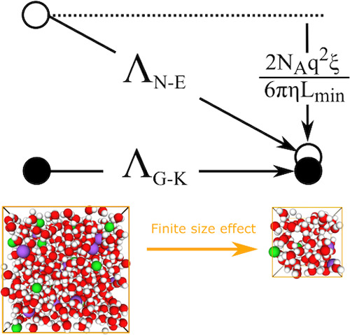
In this work, we used the finite-size effect in molecular dynamics (MD) simulation of transport properties to investigate the deviation from the Nernst–Einstein relation in the case where permanent ion pairing is excluded. It is found that while the Nernst–Einstein conductivity depends strongly on the system size, the Green–Kubo conductivity is system-size independent. We showed that these two types of conductivities crossover at certain simulation box size L_min for both NaCl solutions and [BMIM][PF₆] IL. Furthermore, this observation suggests that the deviation from the Nernst–Einstein relation, i.e., (Λ_N–E – Λ_G–K) is inversely proportional to the viscosity η resembling the classical Walden rule, with L_min being a system-specific parameter. We verified this relation with published experimental data for a variety of ILs. These results indicate that viscosity is a dominating factor for the deviation from the Nernst–Einstein relation and provide a new avenue to gauge the extent of ion–ion correlations in electrolyte systems.

Theoretical Background of Ionic Conductivity

At low salt concentrations, the ionic conductivity of a 1:1 symmetric electrolyte can be described by the Nernst–Einstein (N–E) equation (eq 1), in which the ionic conductivity is only linked to the self-diffusion of ions.¹³

1

2

where β = 1/k_bT is the inverse temperature, q is the formal charge of each ion, and ρ = N/Ω is the number density of the electrolyte (in the formula unit) with Ω as the system volume. σ₊^s and σ_– are contributions to the ionic conductivity from self-diffusion coefficients D₊^s and D_– of cations and anions, respectively.

The Nernst–Einstein relation becomes approximated at high salt concentrations, where the effect of ion–ion cross-correlation starts to show up.^{11,12,14−19} In this case, the ionic conductivity can be formally defined by the Green–Kubo (G–K) formula²⁰

3

4

where J is the total current density and P is the itinerant polarization in ionic solutions²¹ or the Berry phase polarization in solids.^22,23 ⟨···⟩ indicates the ensemble average.

The difference between σ_G–K and σ_N–E can be decomposed into contributions from so-called distinct diffusion coefficients of cations D₊₊^d, anions D_––, and cation–anion D_+–^d.^15,18 The name “distinct” emphasizes the nature of cross-correlation between different ions either in the same species or in different species. Subsequently, this allows rewriting the Green–Kubo conductivity as

5

6

where σ₊₊^d, σ_––, and σ_+–^d are the distinct ionic conductivities from the corresponding distinct diffusion coefficients.

Deviations from the Nernst–Einstein relation, i.e., (σ_N–E – σ_G–K), can be quantified by either experiments or MD simulations. In experiments, they can be obtained as the difference between the pulsed-field gradient NMR and the impedance spectroscopy measurements for the same system under the same conditions.^5,10,24,25 In MD simulations, one can compute σ_G–K using either eqs 3 or 4 and σ_N–E with self-diffusion coefficients obtained from either velocity autocorrelation functions eq 7 or mean squared displacement eq 8.²⁰

7

8

where t is the time, N is the number of cations or anions in solution, α ∈ {+, −}, v_i,α is the velocity of the ith cation or anion, and r_i,α is the corresponding position.

It is worth noting that MD results of σ_N–E obtained by computing self-diffusion coefficients D₊^s and D_– contain a significant finite-size error because of the hydrodynamic self-interaction in periodic systems.^26,27 To obtain the corrected self-diffusion coefficients D_α^s(L → ∞) that are system-size independent, the following formula can be applied.

9

where D_α^s(L) is the self-diffusion coefficient obtained from eq 8 with the box length L, ξ is about 2.837297 for cubic simulation boxes,²⁷ and η is the shear viscosity.

Model Systems and Molecular Dynamics Simulations

Following the spirit of using the ideal potassium chloride (KCl) line for the Walden plot,³ here we took sodium chloride (NaCl) electrolyte solution as a prototype system for aqueous electrolytes. Water molecules were described by the simple point charge/extended (SPC/E) model,²⁸ and Na⁺/Cl^– ions were modeled as point charge plus Lennard-Jones potential using the parameters from Joung and Cheatham,²⁹ which is suitable for highly concentrated solution.³⁰⁻³² The stoichiometry of three different simulation boxes (large, medium, and small) is listed in Section A of the Supporting Information. The molecular dynamics simulations were performed with the LAMMPS code.³³ The sizes of cubic simulation boxes were determined by experimental densities.³⁴ The long-range electrostatics was computed using the particle–particle particle–mesh (PPPM) solver.³⁵ Short-range cutoffs for the van der Waals and Coulomb interactions in direct space are 9.8 Å. For computing ionic conductivities, NVT (constant number of particles, constant volume, and constant temperature) simulations ran for 20 ns with a timestep of 2 fs and trajectories were collected every 0.5 ps. The Bussi–Donadio–Parrinello thermostat³⁶ was used to maintain the given temperature of 20 °C.

Because the [BMIM][PF₆] system does not show permanent ion pairing,³⁷ we picked up this model system in our investigation of ILs here. The interaction model and parameters derived from the OPLS-based force field³⁸ for ILs (OPLS-2009IL)³⁹ were used for the [BMIM][PF₆] system. A charge scaling factor of 0.8e was applied to account for the electronic polarization effects,⁴⁰ which was shown to improve the prediction of self-diffusion coefficients.⁴¹ The stoichiometry of three different simulation boxes (large, medium, and small) is listed in Section B of the Supporting Information. Short-range cutoffs are 13 Å for the [BMIM][PF₆] system. NPT (constant number of particles, constant pressure, and constant temperature) simulations ran for 100 ns with a timestep of 1 fs, and trajectories were collected every 0.5 ps. The Bussi–Donadio–Parrinello thermostat and the Parrinello–Rahman barostat^42,43 were used to maintain the selected temperatures constant and the pressure at 1.0 atm.

Results and Discussion

System-Size Dependence of the Green–Kubo Conductivity

As shown in Figure 1, we found that the ionic conductivities computed using the Green–Kubo formula show no system-size dependence. Such a characteristic is similar to that of the viscosity η, which is also a system-size-independent quantity.²⁷

Figure 1.

Ionic conductivities calculated from the Green–Kubo formula for both (a) NaCl solutions at 20 °C and different concentrations and (b) [BMIM][PF₆] ILs at different temperatures.

Despite that there is no obvious reason why this should be the case, note that both the supercell polarization P used for computing the Green–Kubo conductivity and the pressure tensor p used for computing the viscosity are collective properties of the whole system rather than the average of individual particle’s properties.

With periodic boundary conditions, point charge density and point force density are modified by the compensating background as q_i(δ(r – r_i) – 1/Ω) and F_i(δ(r – r_i) – 1/Ω), respectively. This gives the supercell polarization and the virial part of the pressure as P = ∑_iq_i(δ(r – r_i) – 1/Ω) * r_i and p_v = ∑_iF_i(δ(r – r_i) – 1/Ω) ⊗ r_i. Considering the mathematical similarity between these expressions, it may not be a total surprise that the resulting Green–Kubo conductivity and the viscosity from the linear response theory have the same system-size dependence.

Another angle of looking into this problem may be through the connection between the ionic conductivity σ_G–K and the Maxwell–Stefan diffusion coefficient D_+–^M–S. The Maxwell–Stefan diffusion coefficient D_+– describes the mutual diffusion between cations and anions, which is independent of the reference frame. In binary systems, it is linked to the Green–Kubo conductivity as

10

Recently, it has been proposed that the system-size dependence of the Maxwell–Stefan diffusion coefficient D^M–S in molecular binary mixtures follows the expression⁴⁴

11

Apart from the familiar expression given in eq 9, the new ingredient is the inclusion of the thermodynamic factor Γ as a correction. When Γ is significantly larger than 1, which happens when the two species like to associate with each other, D^M–S becomes effectively system-size independent. What we observed in the case of IL [BMIM][PF₆] may fall into this category, where cations and anions attract each other naturally. However, eq 10 simply does not hold for the case of binary electrolyte solution (cations, anions, and solvent molecules). This makes eq 11 not applicable to NaCl solutions. Moreover, the thermodynamic factor calculated from the experimental mean activity coefficient is not much larger than 1 over the whole concentration range of NaCl solutions (see Section C in the Supporting Information), which further indicates that eq 11 may not be suitable to explain Figure 1.

System-Size Dependence of the Distinct Conductivities

As we found that σ_G–K is system-size independent (Figure 1) and we knew that D₊^s and D_– (therefore σ₊^s and σ_–) are system-size dependent (eq 9), these together imply that some if not all of the distinct conductivities in eq 6 should also be system-size dependent.

To verify this, we calculated the distinct conductivities for both NaCl solution and [BMIM][PF₆] IL with different box sizes, and the results are shown in Figure 2. It is found that the distinct conductivity σ₊₊^d of cations (or σ_–– of anions) has a very similar and strong system-size dependence to that of the corresponding σ₊^s (or σ_–) coming from the self-diffusion of ions. These system-size dependencies are more apparent in the case of NaCl solutions than the case of [BMIM][PF₆]. This is likely due to the fact that the viscosities of NaCl solutions are much smaller than those of [BMIM][PF₆] ILs, following the relation in eq 9. In contrast, the cation–anion distinct conductivity σ_+–^d shows little or no system-size dependence.

Figure 2.

System-size dependence of different contributions to Green–Kubo ionic conductivities for NaCl solutions at 20 °C and different concentrations: (a) cation contributions, (b) anion contributions, and (c) cation–anion distinct diffusion contribution; the same for [BMIM][PF₆] ILs at different temperatures: (d) cation contributions, (e) anion contributions, and (f) cation–anion distinct diffusion contribution.

Why do these distinct conductivities have different system-size dependencies? A simple argument would be that it is for the sake of symmetry. Since there are five terms in eq 5, σ₊₊^d (or σ_––) should be paired up with σ₊^s (or σ_–) and this leaves σ_+–^d on its own. In fact, this is not just an intuition. By connecting Onsager’s phenomenological transport equations with the linear response theory,⁴⁵ Schönert showed that the distinct diffusion coefficient and the self-diffusion coefficient have the following general relation for 1:1 electrolytes.

12

where α ∈ {+, −}, β ∈ {+, −}, and Ω_αβ are the barycentric-fixed Onsager coefficients; N_A is the Avogadro constant; and δ_αβ is the Kronecker delta function. A barycentric-fixed reference frame means the velocity of the center of mass of the system is set to zero, which is the most suitable reference frame for MD simulations.

For ILs, these Ω_αβ coefficients are not independent but follow the expression below because of the conservation of momentum.⁴⁵

13

where M₊ and M₂ are the molecular weights of cations and anions, respectively.

Putting eqs 6, 12, and 13 together, one can arrive at the following expression

14

This means σ_+–^d has the same system-size dependence as σ_G–K in the case of ILs. Since σ_G–K is system-size independent, therefore, σ_+– is also system-size independent. This theoretical prediction is exactly what is shown in Figure 2f. Subsequently, eq 14 also indicates that Ω_+–, Ω₊₊, and Ω_–– are all system-size independent quantities.

Nevertheless, one needs to be aware that there is no such simple relation as eq 13 for a solution made of simple salt and solvent, e.g., NaCl solutions. Therefore, similar behavior of σ_+–^d shown for NaCl solutions in Figure 2c remains as simulation observations.

Crossover Box Length between the Nernst–Einstein Conductivity and the Green–Kubo Conductivity

It is known that the self-diffusion coefficients have strong system-size dependence (eq 9), and therefore, one would expect that the Nernst–Einstein ionic conductivity has the same tendency. Indeed, it is the case for both NaCl solutions and [BMIM][PF₆] ILs as shown in Figure 3.

Figure 3.

Comparison between the system-size dependent Nernst–Einstein ionic conductivity and the Green–Kubo ionic conductivity: (a) NaCl solutions at 20 °C and different concentrations and (b) [BMIM][PF₆] ILs at different temperatures.

What is interesting is that for a small enough simulation box, there exists a crossover box length between the Nernst–Einstein ionic conductivity σ_N–E and the Green–Kubo ionic conductivity σ_G–K. This is clearly seen in both cases of NaCl solutions and [BMIM][PF₆] ILs. The corresponding crossover box length for NaCl solutions is 12.3 Å, and it is 18.0 Å for [BMIM][PF₆] ILs.

Of course, one would immediately argue that the actual crossover box length depends on the force field used even for the same type of systems. However, this is not the question that we will dwell on in this work. Instead, the question that matters here is: Can this crossover between σ_N–E and σ_G–K be always achieved? Supposing that all cations and anions in the system are paired up permanently, then σ_G–K will be absolutely zero, while σ_N–E is not. In other words, if the system has permanent ion pairing, then the crossover between σ_N–E and σ_G–K will never happen. Therefore, we restrict our following discussions to the cases where there is no permanent ion pairing.

Implication of the Crossover Box Length for Ion Transport in ILs

The system-size dependence as discussed in previous sections is usually considered as a finite-size error that needs to be corrected. However, here we turn the tables and use it as a tool instead to investigate the role of viscosity in deviation from the Nernst–Einstein relation.

The observation of the system-size independence of σ_G–K and the crossover box length L_min implies that

15

Combining eqs 1 and 9, one can get

16

Inserting eq 15 into eq 16, one arrives at the following expression

17

Since Λ = σ/c with c as the molar concentration and c = ρ/N_A, the above equation in terms of the molar conductivity Λ can be expressed as

18

Equation 18 suggests that deviations from the Nernst–Einstein relation have a linear relation with respect to 1/η. In other words, it states that the system with a high viscosity will have a small deviation from the Nernst–Einstein relation or vice versa. Furthermore, it has not escaped our notice that eq 18 is reminiscent of the well-known Walden rule Λη = k.⁴⁶

Note that L_min depends on the specific system. For the prototype systems NaCl and [BMIM][PF₆] used here, L_min values are about 12.3 and 18.0 Å, respectively. We notice that L_min/2 for NaCl solutions is about 6.1 Å, which is close to the Kirkwood correlation length in bulk liquid water.⁴⁷

Then, it is exciting to know what the boundaries set by these prototype systems would look like according to eq 18 when compared to experiments. For this purpose, we took a few of seminal experimental studies on ILs, which promoted the idea of ionicity^5,24,25 and made the following mapping: Λ_N–E(L → ∞) ↔ Λ_NMR and Λ_G–K ↔ Λ_Imp. This leads to the results shown in Figure 4.

Figure 4.

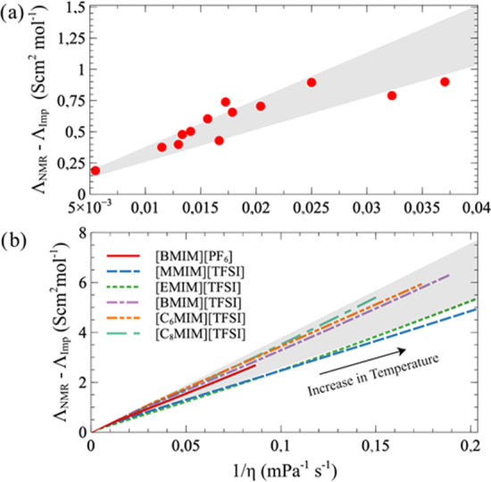
(a) Experimental deviation from the Nernst–Einstein relation for 13 types of ILs extracted from ref (5), together with the theoretical boundaries (gray area) set by prototype systems NaCl and [BMIM][PF₆] using eq 18. (b) Experimental deviation from the Nernst–Einstein relation for 6 types of ILs at various temperatures using fitting coefficients of VFT equations from refs (24, 25), together with the theoretical boundaries (gray area) set by prototype systems NaCl and [BMIM][PF₆] using eq 18.

Figure 4a contains 13 different types of ILs measured at 30 °C (see Table 1 in ref (5) and the list of names in Section D of the Supporting Information), and in Figure 4b, the temperature dependence of molar conductivities and viscosities of 6 types of ILs were measured experimentally and fitted to Vogel–Fulcher–Tammann (VFT) equations.^24,25 It is interesting to see that most experimental data and lines fall into the boundaries set by NaCl and [BMIM][PF₆] and follow eq 18. Since we now know that the value of L_min depends on the specific system under the investigation, this agreement is somehow fortuitous.

Furthermore, we notice that the corresponding L_min/2 follows the order [MMIM][TFSI] > [EMIM][TFSI] > [BMIM][TFSI] > [C₆MIM][TFSI] > [C₈MIM][TFSI], which is in reverse to the alkyl chain length. This suggests that L_min/2 should be regarded as an effective ion–ion correlation length that goes down as the size of the cation becomes larger, following the attenuation of electrostatic interactions. Alternatively, this trend may originate from the reduction of the dielectric constant of the corresponding ILs with an increase of the alkyl chain. Verifying these implications should be the topics of future studies.

Before closing this section, it is necessary to make a connection to the quantities related to the ionicity in ILs. For example, the deviation in ionicity Δ.¹⁰

19

According to the Stokes–Einstein relation, Λ_N–E can be expressed as follows.

20

where r₊ and r_– are the hydrodynamic radii for cations and anions, respectively. r̅ is the mean hydrodynamic radius.

Combining eqs 18, 19, and 20, one arrives at a succinct expression of Δ.

21

As shown in eq 21, Δ does not explicitly depend on the temperature and the pressure. Therefore, one would expect Δ to be a constant for one specific system. This agrees with the experimental pieces of evidence.^11,48

When Δ = 1, this implies that Λ_G–K = 0 and L_min is about 3 times of the mean hydrodynamic radius of ions (see the text around eq 9 regarding the constant ξ). Note that in this limit, eq 9 is no longer applicable.⁴⁹ This in turn suggests that Δ = 1 limit will never be met when permanent ion pairing is not considered. On the other hand, when Δ = 0, this means that Λ_N–E simply equals to Λ_G–K, regardless of the system size. For the infinite dilute solution, this means the correlation length will diverge and L_min → ∞.

Conclusions

The system-size dependence of the Nernst–Einstein conductivity σ_N–E and the Green–Kubo conductivity σ_G–K in NaCl solutions and [BMIM][PF₆] IL was investigated using MD simulations. It is found that σ_N–E is strongly system-size dependent as expected, while σ_G–K does not depend on the system size.

By analyzing the contributions from the distinct diffusion coefficient we further showed that σ_+,–^d between cations and anions have the same system-size dependence as σ_G–K, which is exact for the case of ILs and effective for electrolyte solutions.

Due to different system-size dependencies of the Nernst–Einstein conductivity and the Green–Kubo conductivity, there exists a crossover box length where these two types of conductivities become effectively the same. This leads to an expression for the deviation from the Nernst–Einstein relation (Λ_N–E – Λ_G–K), showing that a low viscosity leads to a strong deviation and a high viscosity leads to a weak deviation (for systems without permanent cation–anion associations), following eq 18.

This new expression was verified against published experimental data of different types of ILs and the system-specific crossover box length L_min may provide a new avenue to gauge the ion–ion correlation in the electrolyte system. Future studies should focus on extending the current formulation to the cases that contain permanent ion pairing and investigating the relationship between the hydrodynamic radius of ions, the L_min, and nano-scale confinement.

Supporting Information Available

The Supporting Information is available free of charge at https://pubs.acs.org/doi/10.1021/acs.jpcb.0c02544.

• Stoichiometry of simulation boxes for NaCl solutions at 20 °C and different concentrations and for [BMIM][PF₆] ILs at different temperatures; thermodynamic factor of NaCl solutions; and the name list of 13 ILs shown in Figure 4a (PDF)

The authors declare no competing financial interest.

References

- Bockris J. O’M.; Reddy A. K. N.; Gamboa-Aldeco M.. Modern Electrochemistry; Kluwer Academic/Plenum Publishers: New York, 2000. [Google Scholar]
- Fawcett W. R.Liquids, Solutions, and Interfaces: From Classical Macroscopic Descriptions to Modern Microscopic Details; Oxford University Press: Oxford, New York, 2004. [Google Scholar]
- Yoshizawa M.; Xu W.; Angell C. A. Ionic Liquids by Proton Transfer: Vapor Pressure, Conductivity, and the Relevance of ΔpKa from Aqueous Solutions. J. Am. Chem. Soc. 2003, 125, 15411–15419. 10.1021/ja035783d. [DOI] [PubMed] [Google Scholar]
- Noda A.; Hayamizu K.; Watanabe M. Pulsed-Gradient Spin-Echo 1H and 19F NMR Ionic Diffusion Coefficient, Viscosity, and Ionic Conductivity of Non-Chloroaluminate Room-Temperature Ionic Liquids. J. Phys. Chem. B 2001, 105, 4603–4610. 10.1021/jp004132q. [DOI] [Google Scholar]
- Tokuda H.; Tsuzuki S.; Susan M. A. B. H.; Hayamizu K.; Watanabe M. How Ionic Are Room-Temperature Ionic Liquids? An Indicator of the Physicochemical Properties. J. Phys. Chem. B 2006, 110, 19593–19600. 10.1021/jp064159v. [DOI] [PubMed] [Google Scholar]
- Ueno K.; Tokuda H.; Watanabe M. Ionicity in Ionic Liquids: Correlation with Ionic Structure and Physicochemical Properties. Phys. Chem. Chem. Phys. 2010, 12, 1649–1658. 10.1039/b921462n. [DOI] [PubMed] [Google Scholar]
- Hollóczki O.; Malberg F.; Welton T.; Kirchner B. On the Origin of Ionicity in Ionic Liquids. Ion Pairing Versus Charge Transfer. Phys. Chem. Chem. Phys. 2014, 16, 16880–16890. 10.1039/C4CP01177E. [DOI] [PubMed] [Google Scholar]
- Kirchner B.; Malberg F.; Firaha D. S.; Hollóczki O. Ion Pairing in Ionic Liquids. J. Phys.: Condens. Matter 2015, 27, 463002 10.1088/0953-8984/27/46/463002. [DOI] [PubMed] [Google Scholar]
- Dokko K.; Watanabe D.; Ugata Y.; Thomas M. L.; Tsuzuki S.; Shinoda W.; Hashimoto K.; Ueno K.; Umebayashi Y.; Watanabe M. Direct Evidence for Li Ion Hopping Conduction in Highly Concentrated Sulfolane-Based Liquid Electrolytes. J. Phys. Chem. B 2018, 122, 10736–10745. 10.1021/acs.jpcb.8b09439. [DOI] [PubMed] [Google Scholar]
- MacFarlane D. R.; Forsyth M.; Izgorodina E. I.; Abbott A. P.; Annat G.; Fraser K. On the Concept of Ionicity in Ionic Liquids. Phys. Chem. Chem. Phys. 2009, 11, 4962–4967. 10.1039/b900201d. [DOI] [PubMed] [Google Scholar]
- Harris K. R. Relations between the Fractional Stokes-Einstein and Nernst-Einstein Equations and Velocity Correlation Coefficients in Ionic Liquids and Molten Salts. J. Phys. Chem. B 2010, 114, 9572–9577. 10.1021/jp102687r. [DOI] [PubMed] [Google Scholar]
- Hansen J.-P.; McDonald I. R. Statistical Mechanics of Dense Ionized Matter. IV. Density and Charge Fluctuations in a Simple Molten Salt. Phys. Rev. A 1975, 11, 2111–2123. 10.1103/PhysRevA.11.2111. [DOI] [Google Scholar]
- Nitzan A.Chemical Dynamics in Condensed Phases: Relaxation, Transfer and Reactions in Condensed Molecular Systems; Oxford Graduate Texts; Oxford University Press: Oxford, New York, 2006. [Google Scholar]
- Altenberger A. R.; Friedman H. L. Theory of Conductance and Related Isothermal Transport Coefficients in Electrolytes. J. Chem. Phys. 1983, 78, 4162–4173. 10.1063/1.445093. [DOI] [Google Scholar]
- Zhong E. C.; Friedman H. L. Self-Diffusion and Distinct Diffusion of Ions in Solution. J. Phys. Chem. A 1988, 92, 1685–1692. 10.1021/j100317a059. [DOI] [Google Scholar]
- Padró J.; Trullàs J.; Sesé G. Computer Simulation Study of the Dynamic Cross-Correlations in Liquids. Mol. Phys. 1991, 72, 1035–1049. 10.1080/00268979100100761. [DOI] [Google Scholar]
- Chowdhuri S.; Chandra A. Molecular Dynamics Simulations of Aqueous NaCl and KCl Solutions: Effects of Ion Concentration on the Single-Particle, Pair, and Collective Dynamical Properties of Ions and Water Molecules. J. Chem. Phys. 2001, 115, 3732–3741. 10.1063/1.1387447. [DOI] [Google Scholar]
- Kashyap H. K.; Annapureddy H. V. R.; Raineri F. O.; Margulis C. J. How Is Charge Transport Different in Ionic Liquids and Electrolyte Solutions?. J. Phys. Chem. B 2011, 115, 13212–13221. 10.1021/jp204182c. [DOI] [PubMed] [Google Scholar]
- Hansen J.-P.; McDonald I. R.. Theory of Simple Liquids; Elsevier: Oxford, U.K., 2013; pp 403–454. [Google Scholar]
- Allen M. P.; Tildesley D. J.. Computer Simulation of Liquids: Second Edition; Oxford University Press: Oxford, U.K., 2017. [Google Scholar]
- Caillol J.-M. Comments on the Numerical Simulations of Electrolytes in Periodic Boundary Conditions. J. Chem. Phys. 1994, 101, 6080–6090. 10.1063/1.468422. [DOI] [Google Scholar]
- King-Smith R.; Vanderbilt D. Theory of Polarization of Crystalline Solids. Phys. Rev. B 1993, 47, 1651–1654. 10.1103/PhysRevB.47.1651. [DOI] [PubMed] [Google Scholar]
- Resta R. Quantum-Mechanical Position Operator in Extended Systems. Phys. Rev. Lett. 1998, 80, 1800–1803. 10.1103/PhysRevLett.80.1800. [DOI] [PubMed] [Google Scholar]
- Tokuda H.; Hayamizu K.; Ishii K.; Susan M. A. B. H.; Watanabe M. Physicochemical Properties and Structures of Room Temperature Ionic Liquids. 2. Variation of Alkyl Chain Length in Imidazolium Cation. J. Phys. Chem. B 2005, 109, 6103–6110. 10.1021/jp044626d. [DOI] [PubMed] [Google Scholar]
- Tokuda H.; Ishii K.; Susan M. A. B. H.; Tsuzuki S.; Hayamizu K.; Watanabe M. Physicochemical Properties and Structures of Room-Temperature Ionic Liquids. 3. Variation of Cationic Structures. J. Phys. Chem. B 2006, 110, 2833–2839. 10.1021/jp053396f. [DOI] [PubMed] [Google Scholar]
- Dünweg B.; Kremer K. Molecular Dynamics Simulation of a Polymer Chain in Solution. J. Chem. Phys. 1993, 99, 6983–6997. 10.1063/1.465445. [DOI] [Google Scholar]
- Yeh I.-C.; Hummer G. System-Size Dependence of Diffusion Coefficients and Viscosities from Molecular Dynamics Simulations with Periodic Boundary Conditions. J. Phys. Chem. B 2004, 108, 15873–15879. 10.1021/jp0477147. [DOI] [Google Scholar]
- Berendsen H. J. C.; Grigera J. R.; Straatsma T. P. The Missing Term in Effective Pair Potentials. J. Phys. Chem. C 1987, 91, 6269–6271. 10.1021/j100308a038. [DOI] [Google Scholar]
- Joung I. S.; Cheatham T. E. Determination of Alkali and Halide Monovalent Ion Parameters for Use in Explicitly Solvated Biomolecular Simulations. J. Phys. Chem. B 2008, 112, 9020–9041. 10.1021/jp8001614. [DOI] [PMC free article] [PubMed] [Google Scholar]
- Zhang C.; Raugei S.; Eisenberg B.; Carloni P. Molecular Dynamics in Physiological Solutions: Force Fields, Alkali Metal Ions, and Ionic Strength. J. Chem. Theory Comput. 2010, 6, 2167–2175. 10.1021/ct9006579. [DOI] [PubMed] [Google Scholar]
- Yllö A.; Zhang C. Experimental and Molecular Dynamics Study of the Ionic Conductivity in Aqueous LiCl Electrolytes. Chem. Phys. Lett. 2019, 729, 6–10. 10.1016/j.cplett.2019.05.004. [DOI] [Google Scholar]
- Nezbeda I.; Moučka F.; Smith W. R. Recent Progress in Molecular Simulation of Aqueous Electrolytes: Force Fields, Chemical Potentials and Solubility. Mol. Phys. 2016, 114, 1665–1690. 10.1080/00268976.2016.1165296. [DOI] [Google Scholar]
- Plimpton S. Fast Parallel Algorithms for Short-Range Molecular Dynamics. J. Comput. Phys. 1995, 117, 1–19. 10.1006/jcph.1995.1039. [DOI] [Google Scholar]
- Rumble J.CRC Handbook of Chemistry and Physics; CRC Press: Boca Raton, FL, 2018. [Google Scholar]
- Hockney R. W.; Eastwood J. W.. Computer Simulation Using Particles; CRC Press: New York, 1988. [Google Scholar]
- Bussi G.; Donadio D.; Parrinello M. Canonical Sampling Through Velocity Rescaling. J. Chem. Phys. 2007, 126, 014101 10.1063/1.2408420. [DOI] [PubMed] [Google Scholar]
- Zhao W.; Leroy F.; Heggen B.; Zahn S.; Kirchner B.; Balasubramanian S.; Müller-Plathe F. Are There Stable Ion-Pairs in Room-Temperature Ionic Liquids? Molecular Dynamics Simulations of 1-n-Butyl-3-methylimidazolium Hexafluorophosphate. J. Am. Chem. Soc. 2009, 131, 15825–15833. 10.1021/ja906337p. [DOI] [PubMed] [Google Scholar]
- Jorgensen W. L.; Maxwell D. S.; Tirado-Rives J. Development and Testing of the OPLS All-Atom Force Field on Conformational Energetics and Properties of Organic Liquids. J. Am. Chem. Soc. 1996, 118, 11225–11236. 10.1021/ja9621760. [DOI] [Google Scholar]
- Sambasivarao S. V.; Acevedo O. Development of OPLS-AA Force Field Parameters for 68 Unique Ionic Liquids. J. Chem. Theory Comput. 2009, 5, 1038–1050. 10.1021/ct900009a. [DOI] [PubMed] [Google Scholar]
- Kirby B. J.; Jungwirth P. Charge Scaling Manifesto: A Way of Reconciling the Inherently Macroscopic and Microscopic Natures of Molecular Simulations. J. Phys. Chem. Lett. 2019, 10, 7531–7536. 10.1021/acs.jpclett.9b02652. [DOI] [PubMed] [Google Scholar]
- Doherty B.; Zhong X.; Gathiaka S.; Li B.; Acevedo O. Revisiting OPLS Force Field Parameters for Ionic Liquid Simulations. J. Chem. Theory Comput. 2017, 13, 6131–6145. 10.1021/acs.jctc.7b00520. [DOI] [PubMed] [Google Scholar]
- Shinoda W.; Shiga M.; Mikami M. Rapid Estimation of Elastic Constants by Molecular Dynamics Simulation under Constant Stress. Phys. Rev. B 2004, 69, 134103 10.1103/PhysRevB.69.134103. [DOI] [Google Scholar]
- Parrinello M.; Rahman A. Polymorphic Transitions in Single Crystals: A New Molecular Dynamics Method. J. Appl. Phys. 1981, 52, 7182–7190. 10.1063/1.328693. [DOI] [Google Scholar]
- Jamali S. H.; Wolff L.; Becker T. M.; Bardow A.; Vlugt T. J. H.; Moultos O. A. Finite-Size Effects of Binary Mutual Diffusion Coefficients from Molecular Dynamics. J. Chem. Theory Comput. 2018, 14, 2667–2677. 10.1021/acs.jctc.8b00170. [DOI] [PMC free article] [PubMed] [Google Scholar]
- Schoenert H. Evaluation of Velocity Correlation Coefficients from Experimental Transport Data in Electrolytic Systems. J. Phys. Chem. D 1984, 88, 3359–3363. 10.1021/j150659a045. [DOI] [Google Scholar]
- Walden P. Über organische Lösungs- und Ionisierungsmittel. Z. Phys. Chem. 1906, 55U, 207–249. 10.1515/zpch-1906-5511. [DOI] [Google Scholar]
- Zhang C.; Hutter J.; Sprik M. Computing the Kirkwood g-Factor by Combining Constant Maxwell Electric Field and Electric Displacement Simulations: Application to the Dielectric Constant of Liquid Water. J. Phys. Chem. Lett. 2016, 7, 2696–2701. 10.1021/acs.jpclett.6b01127. [DOI] [PubMed] [Google Scholar]
- Harris K. R. Can the Transport Properties of Molten Salts and Ionic Liquids Be Used To Determine Ion Association?. J. Phys. Chem. B 2016, 120, 12135–12147. 10.1021/acs.jpcb.6b08381. [DOI] [PubMed] [Google Scholar]
- Hasimoto H. On the Periodic Fundamental Solutions of the Stokes Equations and Their Application to Viscous Flow Past a Cubic Array of Spheres. J. Fluid Mech. 1959, 5, 317–328. 10.1017/S0022112059000222. [DOI] [Google Scholar]
Associated Data
This section collects any data citations, data availability statements, or supplementary materials included in this article.