Particle and Size Distribution

Abstract

The purpose of air cleaning technology is to get rid of airborne particles as much as possible. Gaseous medium containing dispersed airborne particles is one kind of dispersed systems, which is termed as aerosol.

The purpose of air cleaning technology is to get rid of airborne particles as much as possible. Gaseous medium containing dispersed airborne particles is one kind of dispersed systems, which is termed as aerosol.

Exactly speaking, according to ISO definition [1], aerosol system is “the airborne system in gases containing solid particle, liquid particle or solid/liquid particle whose settling velocity could be ignored.”

The way that how airborne particles move and distribution is fundamental to air cleaning technology. In order to illustrate easily, particles and size distribution characteristics will be introduced firstly and how particles move indoors in the following chapters.

Particle Classification

Classification with Particle Formation Methods

1. Dispersed Particles. They are formed into airborne state from solid/liquid under the effect of division, collapse, flow stream, and vibration. Solid dispersed particles could be those with irregular shape or those formed by loosely coagulated particles.

2. Coagulated Particles. They are formed by the process of combustion, sublimation, vapor condensation, and gas reaction. Solid coagulated particles are usually formed by many loose coagulated groups from primary particles with regular crystallization shape or spherical shape. Liquid coagulated particles are smaller than liquid dispersed particles, and the extent of their polydispersity is smaller.

Classification with Particle Origin

1. Inorganic Particles. Such as metal dust particle, mineral dust particle, and particles from construction materials

2. Organic Particles. Such as plant fibers, animal skin, hair, horniness, skin debris, chemical fuel, and plastic

3. Living Particles. Such as unicellular algae, fungi, protozoa, bacteria, and virus

Classification with Particle Size

The size range of aerosol is 10⁻⁷ to 10⁻¹ cm, and within this range, the physical characteristic and law will be different when particle size changes.

1. Visible Particle. Visible with eyes and the corresponding particle diameter is larger than 10 μm.

2. Microscopic Particle. Visible with the microscope and the corresponding particle diameter is 0.25–10 μm.

3. Supermicroscopic Particle. Visible with supermicroscope or electronic microscope and the corresponding particle diameter is smaller than 0.25 μm.

It should be noted that particles with diameter 0.1–5 μm are classified as fine particles; those <0.1 μm are superfine particles, and those >5 μm are big particles.

Common Classification Method

In the technical field of aerosol, terms as “dust,” “smoke,” and “mist” are frequently used. Some definition and concept in air cleaning technology are also usually referred to these terms (such as “dust” concentration in the air and oil “mist” meter). These are the common classifications for particles:

1. Dust. It includes all the solid dispersed particles. The movement of these particles in the air is influenced by the combined effect of gravity and diffusion. It is almost ubiquitous in air cleaning technology.

2. Smoke. It includes solid coagulated particles, particles formed by coagulation effect from liquid and solid particles, and particles from the transition from liquid particle to crystallized particle.

According to ISO definition, smoke is clearly defined as “aerosol formed by solid particles during the metallurgy process. It is the gaseous condensate from the vapor generated after the evaporation of melted material. During the formation process, chemical reaction such as oxidation usually occurs.” In the usual circumstance, particles from smoke with diameters much less than 0.5 μm are mainly controlled by Brownian motion effect in the air, which makes the particles strong disperse capacity, and they are difficult to settle down in still air. Smoke stream generated by smoke generator is usually used to detect the leakage on air filters in air cleaning technology field and to perform the experiment for the flow visualization.

• 3.Fog and haze. Fog includes all the dispersed liquid particles and coagulated liquid particles.

According to ISO definition, mist means “the general term for liquid airborne system in air. In meteorology field it means the airborne system containing droplets which causes the visibility length less than 1 km.” Particle size differs with formation state, and it is between 0.1 and 10 μm. Stokes law mainly dominates their movement. For example, sulfate mist generated from SO₂ gas will be transformed into oil mist by the combined effect of heat and compressed air, and oil mist could be the standard aerosol for testing air filter. The combination of fog and fine solid particles is termed as haze.

• 4.Smog. It includes both liquid and solid particles and both dispersed and coagulated particles. The size ranges from several tenth micrometers to dozens micrometers, such as the combined system formed by coal dust, SO₂, CO, and water vapor, which exist in the air of industrial zone (the typical case is the London mist which is the mixture of smoke and mist, and the FeO smog generated in iron plant). However, according to ISO definition, smog usually represents “visible aerosol generated during combustion process” and “no water vapor included,” which means there is a little difference between smog and mist.

Figure 1.1 illustrates the size and range of aerosol particles.

Fig. 1.1.

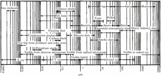
Size range of particles

Evaluation of Particle Scale

Particle Size

Particle size is usually used to represent how big the particle is. However, not all the particles, especially dust particles, have regular geometric shape such as spherical or cubic. Therefore the term “particle size” used frequently does not mean the real diameter of sphere. In the field of aerosol and air cleaning technology, the meaning of “particle size” is some length dimension inside particles, without indication of the meaning of regular geometric shape. When particle scale is analyzed, “particle size” does have this indication.

Exactly speaking, particle size could be divided into two categories:

The first one was measured and defined according to particle’s geometric characteristic, such as microscopic method used to determine the particle size. For example, when particles were observed with optical microscopic after the dust sampling, the dust sample was moved towards one direction and through micrometer, where particle was projected onto this scale meter, and the length between two cutting edges by the meter represents the particle size. Particles were measured in a sequential and random way, so the long length was determined when the longer side of particle approached, and the short length was measured when the shorter side approached (shown in Fig. 1.2).

Fig. 1.2.

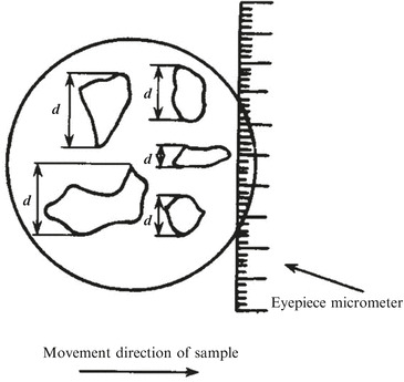
One method to determine particle size

The long and short sides were called directional tangential cutting edge or random diameter. When the number of measured particles was large enough, results could reflect the average cross section of particle sample properly. In this way, it is convenient to take measurements. However, in some cases only the maximum projected distance was adopted as particle diameter, such as several standards about cleanroom in the USA. Obviously micrometer must be rotated during measurement, and the location for maximum distance could not be fixed precisely. So the Japanese standard “Measurement of Airborne Particles in Cleanroom” (Japanese Industrial Standards, JIS) suggests no need to rotate micrometer, and instead only the projected maximum length is estimated, which was thought to cause small error. For cubic particles, the diagonal is also used to represent particle size, so it equals with the multiplication of the side length and . For particles whose projected area is rectangular, the average of long and short side lengths is used, and also the diagonal length could be used based on the short side length. In the following paragraph, NaCl particles will be introduced, and particle size determined by diagonal method is used since the projected area of their crystal is usually quadrate.

The other group was based on the indirect measurement and definition of some physical property of particles. Precipitation method and optic-electrical method are used to determine the particle size. The value obtained is actually an equivalent diameter. In the former Federal German Standard VDI-2083, particle size was defined as the equivalent diameter according to the measuring method, which means some physical property and parameter of referenced particles are equivalent with the counterparts of these particle cloud based on this diameter value. For example, when light scattering air particle counters are used, “particle size” represents the comprehensive effect, i.e., the geometric size range, by comparing the equivalent light scattering intensity between the tested particle and standard particle (such as PSL particles). Setting velocity of particles could be measured, and when the settling velocity in still air calculated by Stokes law in 10.1007/978-3-642-39374-7_6 is equal to that of particles with same density, the spherical diameter of latter is called settling diameter, also Stokes diameter, which is labeled as d _st, and it is smaller than other diameter value. Assume the density is 1, the diameter of spherical particles whose settling velocity is the same will also be called aerodynamic diameter, which is widely used in environmental science and labeled as d _a. It is known from 10.1007/978-3-642-39374-7_6) that . So the following correlation can be obtained:

1.1

where ρ _P represents the particle density.

American Federal Standards 209C and 209E allowed to use either of (1) maximum visible linear length of particle or of (2) equivalent diameter measured by automatic meter.

Average Particle Size

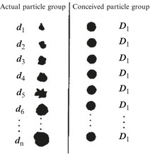
Since particle shape differs a lot from each other, different values of particle size could be obtained with the above methods, which is inconvenient for application. Therefore, one method to reflect some characteristic by the average particle size from all the particles must be found, and the average value is called “average particle size.” This special method is used to represent a hypothesized particle diameter according to some certain characteristic.

Assume the actual particle sizes are d ₁, d ₂, …, d _n, respectively, which is shown in Fig.1.3. These values of particle size were determined by the before-mentioned method. Some certain characteristic (such as light scattering property) could be represented by f(d ₁), f(d ₂),…, f(d _n), so the property of the particle group f(d) has the following relationship with that of individual particle:

1.2

Fig. 1.3.

Conceived particle group and average particle size

Suppose another particle group contains particles with the same particle size D and its property (such as light scattering property) is the same as that of the actual particle group, so we could get

1.3

where the particle size D means the average particle size of this particle group corresponding to some certain property. D could be defined as the side length of the hexahedron or the diameter of sphere. The latter is usually used, which means the particle group could be treated as a group of spheres with the same diameter.

The simplest case is to assume that the group consists of particles with the same diameter D ₁, so the total length of all diameters is the same as that of actual particle group. According to Eq. (1.3), we could obtain

1.4

This is the arithmetic average diameter. In this equation, d _i is the particle size by any measuring method; m _i is the number of particles with diameter d _i; n is the total particle number.

If the summation of assumed particle areas (projected area or surface area) is the same as that of the actual particle group, we could get the following equation based on Eq. (1.3):

1.5

This diameter is termed as average surface diameter.

If the specific length area (i.e., the cross section area per unit length) of the assumed particle group is the same as that of the actual particle group, we could get the following derivation:

or

Hence

1.6

This diameter is termed as specific length diameter.

The same method could be utilized to obtain other average diameters. The cross section could be circular (sphere) or rectangular. Moreover, average diameter could be determined according to the particle size frequency distribution. Table 1.1 lists these average diameters.

Table 1.1.

Average diameter of particles

Symbol	Term	Significance	Calculation method
D mod	Model diameter (or population diameter)	The diameter corresponding with the maximum proportion in the samples. The minimum diameter calculated with the frequency distribution	Obtained from the summit on the distribution curve of particle frequency
D 50 or D m	Medium diameter	The number of particles with diameter lager than this value is the same as that with diameter less, and this is called the number medium diameter. The mass of particles with diameter lager than this value is the same as that with diameter less, and this is called the mass medium diameter. All the diameters related to the number are smaller than that related to mass	Obtained at 50 % of the cumulative distribution curve of particle number (or mass)
or D 1	Arithmetic average diameter	It is a kind of arithmetic average values and is the habitually most popular diameter. But small particles occupy the majority in the particle group. So even though the mass may be small, the calculated average diameter will also be greatly reduced. So there is great limit between the real size of particle group and the physical property of this particle group	, where n i is the particle number at each size and Σn i is the total particle number
D 2	Specific length diameter (length weighted)	It is the division between the projected particle area and the summation of diameters, which is the average diameter per unit length
D 3	Specific area diameter (area weighted)	It is the division of the total volume of particles to the summation of cross-sectional area, which is the average diameter per unit area
D 4	Specific mass diameter (mass weighted, volume weighted)	It is obtained with the surface area per unit mass, namely, the average diameter of unit mass (or volume). It is larger than any other diameter
D S	Average area diameter	It is the area weighted diameter according to the particle number
D V	Average volume (or mass) diameter	It is the volume (or mass) weighted diameter according to the particle number
D g	Geometric mean diameter		●
		It is the average of the logarithmic diameters	● Expressed with natural logarithm
		Or it is the nth root of the multiplication of several values
		Or it is the diameter with the maximum frequency from the lognormal distribution, and it is equal with the medium diameter of the particle number. It is always equal to or less than the arithmetic average diameter	● For unclassified data
			● For classified data
			so
			or
			● The summit point can be obtained from the lognormal distribution curve

By comparison of these diameters, we could get the following sequence:

It should be noted for the average particle size names listed in the table. In literature, terms with converse sequence could be encountered. For example, some use “average area diameter,” while others use “area average diameter.” Therefore, the meaning could be clearly understood only when the expression is known. But if we start from the definition, it’s easier to understand the meaning. For example, in Table 1.1, “average area” obviously means all the areas averaged by some quantity (such as particle number), so the area is in the numerator. “Area weighted” (“specific area”) obviously means per unit area, so the area is in the denominator. As long as we keep in mind of this standard, we will not be confused. As for which average diameter is reasonable, it depends on the purpose of the work. If the gravimetric method is used to measure the particle concentration, diameter D _v which is related to mass should obviously adopted; when the property of light scattering is under investigation, it’s better to use average area diameter D _s or average volume diameter D _v, because for different particle size range, the quantity of light scattering probably depends on the particle area or volume; when the problem is related to the light refraction property, arithmetic average diameter D ₁ should be used, because this property depends on the dimension of particle length.

Now let’s calculate the average diameter of particles.

During the measurement of particle concentration with the sodium flame method, electronic microscopic could be used to measure the short side length of NaCl particles from 823 samples obtained from the supply air, and we assume the amplification ratio is 30,000 (i.e., include the amplification ratio of electric glass and amplification ratio of reader microscopic for reading values on SEM figures); the lower and upper limits for the group of short side could be calculated by

1.7

where

• d _p is the upper/lower limit of particle size range

• a is the measured value of upper/lower limit of short side

Results for a are as follows:

Particle size interval (μm)	<0.05	0.05–<0.1	0.1–<0.2	0.2–<0.4	0.4–<0.6	0.6–<1.0
a (mm)	<0.87	0.87–<1.7	1.7–<3.5	3.5–<6.9	6.9–<10.4	10.4–<17.3
Number	17	99	429	225	40	13

According to the data from Table 1.2, we could obtain the arithmetic average diameter:

Table 1.2.

Calculation table for average particle diameter

1	2	3	4	5	6	7	8	9	10	11
Particle size interval (μm)	Avg. value, d i	Number, n i	n i d i							Number frequency (%)
<0.05	0.025	17	0.425	0.0625	1.06	0.16	2.72	0.39	6.63	2.06
0.05–<0.1	0.0725	99	7.425	0.5625	55.69	4.23	418.77	31.64	3,132.36	12.03
0.1–<0.2	0.15	429	64.350	2.25	956.25	33.75	14479	506	200,000	52.13
0.2–<0.4	0.3	225	67.500	9	2,025	270	60,750	8,100	1,822,500	27.34
0.4–<0.6	0.5	40	20.000	25	1,000	1,250	50,000	62,500	2,500,000	4.86
0.6–<1.0	0.8	13	10.400	64	832	5,120	66,560	409,600	5,324,800	1.58
∑		823	170.10		48.68		19.2		9.85	100

Specific length diameter

Specific area diameter

Specific mass diameter

Area weighted diameter

Volume weighted diameter

When geometric mean diameter is calculated, we know

Hence we get

Reading on the photoelectric flame photometer used in the sodium flame method is proportional with the mass concentration of sodium chloride. Therefore, it is better to use mass ratio diameter D ₄ to represent average diameter of sodium chloride particles. In the above example, D ₄ = 0.513 μm, while the designated value in foreign standard is 0.6 μm.

Statistical Distribution of Particle Size

A lot of data on particle size will be frequently obtained in the field of air cleaning technology. After sampled on chemical porous membrane, particles with various shapes could be visible with microscope. Different samples will be obtained even though they are sampled simultaneously. Although particles are distributed randomly on the membrane surface, useful “information” is embedded behind those disorderly data. If arrangement and analysis are performed on these data, useful “information” could be extracted fully and correctly, which could be used as the basis for technical measurement adopted in dust measures, dust proof, and dust control. The purpose of data arrangement and analysis is to find the distribution law of particle number with particle size or density. A functional relationship could be used to describe this kind of law. However, there is no special theoretical basis that which kind of law is suitable for particle distribution. It is mainly dependent on experience.

Particle Size Distribution Curve

It is not enough to represent particle characteristic only with calculated average diameter. Particle characteristic depends to a great extent on the law of particle size distribution.

Distribution of particle size also means the dispersity of particles, which represents the number or mass percentage of particles at different size within the group of particle clusters. If particle percentage in the size distribution is introduced with particle number, it is called number frequency distribution (or simplified as frequency distribution). Particle number is usually a big number, so frequency distribution is preferred instead of number distribution in the study of particle size distribution. If particle mass is used for size distribution, it is called mass distribution. If particle surface area is used, it is called surface area distribution. Dispersity of a particle group will be higher for the case of particle cluster with higher percentage of smaller particles and vice versa. Dispersity represents the extent of fragmentation of dispersed material. When dispersity of a particle group is needed, particle size distribution should be obtained.

In the figure of particle size distribution curve, the number of particles within certain range of diameter values, or the ratio (or frequency) of particles in various diameter range segments, will be presented. The curve is obtained by smoothing the frequency distribution in the histogram.

Frequency Distribution (i.e., Relative Frequency Distribution) ΔD (%)

It is described with the percentage ratio of certain physical parameter (e.g., number ΔN) of particles with diameters between D _p and D _p + ΔD _p to the same parameter (e.g., total number ΔN) corresponding to the particle group:

1.8

At first particle diameter is divided into several groups as needed or according to measurement method. It is better to set the diameter distance equally. The upper limit diameter of each group coincides with the lower limit diameter of the neighboring group with lager diameter. If one diameter value equals with the threshold value, it belongs to the larger diameter group. For example, when the diameter group of 0.2–0.4 and 0.4–0.6 are considered, particles with diameter 0.4 μm enters into the second group.

Secondly, particle numbers in each diameter group are countered, and frequency numbers are obtained. When frequency number is plotted as ordinate and diameter as abscissa, histogram could be acquired after rectangles with the height of frequency number are draw. If the ordinate is replaced with frequency (particle number within certain diameter range divided by the whole particle number), the histogram of frequency distribution is acquired.

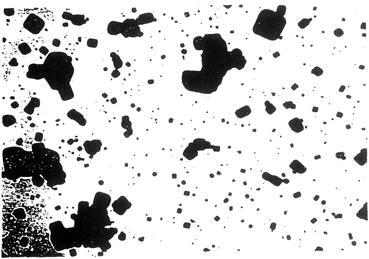
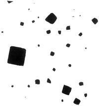
Figure 1.4 is the NaCl aerosol particles used in the sodium flame method. Figure 1.5 illustrates the situation after its sedimentation and coagulation. Figure 1.6 presents the shape after deformation when wetted [2].

Fig. 1.4.

NaCl aerosol particle with magnification of 27,000

Fig. 1.5.

NaCl aerosol particles after sedimentation and coagulation (magnification ratio 13,000)

Fig. 1.6.

NaCl aerosol particles after wet-absorbed deformation (magnification ratio 22,250)

Table 1.3 shows the number of another group of NaCl aerosol particles with SEM figures, from which we could get the number averaged diameter .

Table 1.3.

Number frequency distribution of NaCl aerosol particles

Group (μm)	Frequency	Percentage (%)	Cumulative percentage (%)	Cumulative mass percentage (%)
<0.1	2,895	19.09	19.09	0.11
0.1–<0.2	7,252	47.81	66.90	7.29
0.2–<0.3	2,770	18.26	85.15	19.59
0.3–<0.4	1,314	8.66	93.82	36.52
0.4–<0.5	479	3.16	96.98	49.33
0.5–<0.6	217	1.47	98.41	59.92
0.6–<0.7	116	0.76	99.17	69.25
0.7–<0.8	51	0.34	99.51	75.60
0.8–<0.9	32	0.21	99.72	81.35
0.9–<1.0	14	0.09	99.81	84.88
1.0–<1.1	10	0.06	99.87	88.27
1.1–<1.2	8	0.05	99.92	90.95
1.2–<1.5	8	0.05	99.97	95.28
1.5–<2.0	4	0.03	100.00	100.00

In Table 1.3, the cumulative mass frequency is obtained from the mass frequency distribution which could be calculated by the product of cubic of mean diameter in the diameter range and particle number.

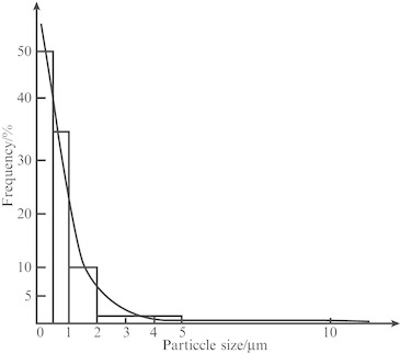
Relative frequency distribution histogram shown in Fig. 1.7 could be depicted by this table, where the dashed line means the fitted particle distribution curve on the histogram.

Fig. 1.7.

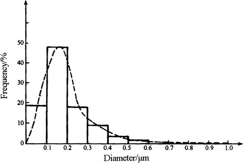
Frequency distribution histogram

Figure 1.8 shows the stereo of NaCl particles [3].

Fig. 1.8.

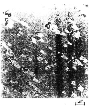
Stereo of NaCl particles

Particle size distribution curves for most particle group are asymmetrical, and they are inclined towards larger diameter. This is almost an intrinsic feature for dust particles since particles with small diameter occupy most portions of the whole dust particles. This kind of distribution is called “right-handed inclination” distribution. Furthermore, there are also “left-handed inclination” distribution and “symmetrical distribution,” which are both presented in Fig. 1.9.

Fig. 1.9.

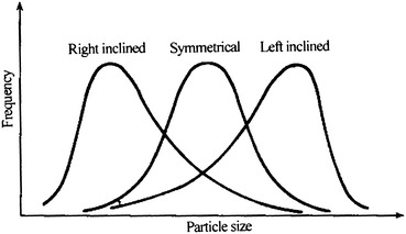
Frequency distribution of particle size

Frequency Distribution (i.e., Frequency Density Distribution) (% · μm⁻¹)

It is described by the frequency distribution corresponding to the unit particle size range (e.g., 1 μm), i.e.,

1.9

When the particle size ranges, especially those in the middle of data, are not equal, the fitted curve from histogram of frequency distribution will not be smooth, and it deviates greatly from the reality.

Take a look at Table 1.4 [4]; we could see the great discrepancy exists between particle size ranges. If histogram is plotted with the frequency data, we could get Fig. 1.10. When the frequency density is used, which is the proportionality of particle number per unit size range, we could obtain the histogram as shown in Fig. 1.11. It is obvious that it is difficult to get any smooth curve for the former case. Even if the dashed line was drawn, it is quite different from the dashed line in the latter.

Table 1.4.

Classified data with larger interval

Interval (μm)	Number frequency (#)	Percentage (%)	Percentage per micrometer, i.e., channel frequency (%)
0–<4	104	10.4	2.6
4–<6	160	16.0	8.0
6–<8	161	16.1	8.05
8–<9	75	7.5	7.5
9–<10	67	6.7	6.7
10–<14	186	18.6	4.56
14–<16	61	6.1	3.05
16–<20	79	7.9	1.98
20–<35	103	10.3	0.69
35–<50	4	0.4	0.027
<50	0	0	0
Total	1,000	100.0

Fig. 1.10.

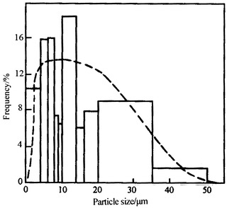
Frequency diagram

Fig. 1.11.

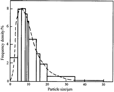
Channel frequency diagram

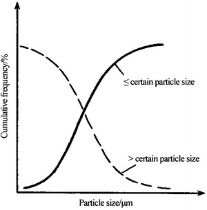
Upper Cumulative Frequency Distribution (Abbreviated as Upper Distribution) R(D) (%)

It is expressed as the percentage of certain parameter of all particles with diameter larger than D _P when compared with the same parameter of whole particle group, i.e.,

1.10

Lower Cumulative Frequency Distribution (Abbreviated as Lower Distribution) D(D) (%)

It is expressed as the percentage of certain parameter of all particles with diameter smaller than D _P when compared with the same parameter of whole particle group, i.e.,

1.11

Figure 1.12 shows a typical curve of cumulative frequency distribution.

Fig. 1.12.

Typical distribution curve of cumulative frequency

Figure 1.13 illustrates the relationship between frequency distribution and upper cumulative frequency distribution. The relationship between frequency distribution and lower cumulative frequency distribution could be derived in a similar way.

Fig. 1.13.

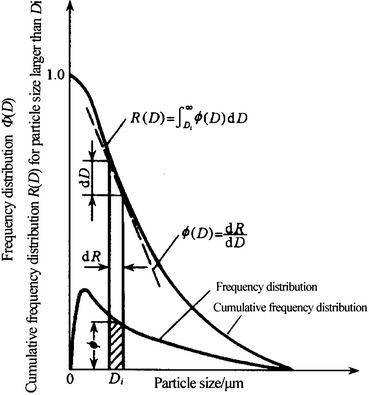
Relationship between frequency distribution and cumulative frequency distribution

Bimodal and Multimode Distribution

For some aerosol particles, there will be two or more than two peak values in the frequency distribution curves. The distribution function is comparatively complex, so it will not be introduced here. Some examples are given for reference.

1. Oil mist aerosol. Oil mist is produced by the processes of oil heating, nozzle spraying, and condensation after evaporation. According to the research report [5], this kind of oil mist aerosol has the feature of bimodal distribution, where the main summit located at the diameter 0.133 μm and the second summit at 0.024 μm. The curve shape is independent of the amount of big particles separated. Figure 1.14 shows the curve shape. The reason to form this kind of bimodal distribution is that there are many components and a few nonvolatile materials in the test oil (turbine oil) and these components have respective distribution summit values.

2. Cold DOP aerosol (which can be seen in 10.1007/978-3-642-39374-7_17#Sec32). It is also called pressurized DOP aerosol, which is the liquid mist sprayed from the Laskin nozzle after compressed air goes through the DOP liquid. According to some research report [6], the generated particles have the characteristic of bimodal distribution, no matter how much the compressed air pressure is. The particle size at valley between two summits is equivalent to the median diameter 0.275 μm. Figure 1.15 shows the frequency distribution measured by the channels of laser optical particle counter (every channel corresponds to a certain particle size range, and in the figure the data of particle size were calculated with the channel data from LAS-x particle counter in the test). It is shown that one channel exists between the second peak and the valley and the second peak value is corresponding to 0.3 μm (median diameter). It should be noted that the above experiment was carried out with the laser particle counter which was able to detect the particles with diameter smaller than 0.1 μm (0.09 μm). If the particle counter with the incandescent light was used and the lower detect limit is 0.3 μm, there would be no bimodal distribution [7], and the resultant number median diameter would obviously be smaller than 0.3 μm, which is different from the above experimental result. Therefore the appearance of bimodal distribution is related to the test method, which needs further investigation.

Fig. 1.14.

Bimodal distribution of oil mist aerosol

Fig. 1.15.

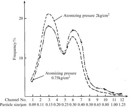
Bimodal distribution of cold DOP aerosol

Normal Distribution and Lognormal Distribution

Normal distribution curve is symmetrical in the middle which is shown in Fig.1.9. There is a highest point in the curve. The curve decreases monotonically towards two sides when the abscissa value of this point is considered as the center. The concept of normal distribution is one of the most important distribution concepts in statistics. In natural and engineering applications, it is the most widely used distribution for continuous data. Now the key points useful for study of particle size distribution will be introduced.

It is known from Figs. 1.9 and 1.10 that a comparatively smooth curve could be obtained from the histogram. Besides, the smooth curve could also be obtained when the sample number increases and the distance of subrange decreases, which is called probability density curve and is usually expressed as

where y means the probability density, which is equal to the frequency value per unit abscissa value, and x means the abscissa value, which is the obtained data.

Normal probability density function could be used to represent the normal distribution curve:

1.12

where

• d _t is the particle size;

• is the average size, and it is usually the arithmetic mean diameter, so in mathematics it is the average value or expectation; for the case of normal distribution, ;

• σ is the standard deviation of a certain particle group. Since particle number of the particle group sample is very large, it could be expressed as

1.13

It is known with calculation that after many times of measurement, the probability for particles with measured diameter in the range of is 68.3 %, and for particles with , it is 95.4 %, while for particles with , it is 99.7 %. At the same time, the value of σ could be used to represent the extent of “slim” for the curve. The curve is “fat” with large value of σ, which means data are scattering and vice versa. Figure 1.16 gives the schematic diagram of both situations.

Fig. 1.16.

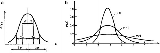
Visual diagram of the meaning of σ (a) Relationship between σ and probability. (b) Relationship between σ and data dispersity

For the case of normal distribution when the abscissa of the highest point on the curve equals with 0 and the standard deviation is 1, it is termed as the standard normal distribution and labeled as N(0, 1). Standard normal distribution curve could be obtained when any nonstandard normal distribution curve is translated, as shown in Fig. 1.17.

Fig. 1.17.

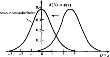
Standard normal distributions

Cumulative distribution function F(x) is obtained by integrating probability density function, and it is as follows:

1.14

or

1.15

Figure 1.17 presents the curve for probability density function, and Fig. 1.18 is its cumulative distribution function curve.

Fig. 1.18.

Curve for cumulative distribution function

The relationship between and F(x) is that of derivative and integration. This is the same for other statistical distribution, and it will be used in the process of sampling and measurement.

One special coordinate paper is called normal probability paper shown in Fig. 1.19, where its abscissa uses normal scale while the ordinate is drawn according to the normal distribution feature. If particle diameters follow normal distribution, a straight line will be obtained when the abscissa represents the particle size and the ordinate means the cumulative distribution frequency. This is one simple method to check whether particle size distribution is normal distribution.

Fig. 1.19.

Normal probability paper

Normal distribution could be used to depict specially generated monodisperse aerosols and pollen particles with single diameter, while most particle diameters do not follow normal distribution but close to it. For the case shown in Fig. 1.11, the cumulative distribution curve on the normal probability paper is not straight as noted in Fig. 1.19. The reasons are:

1. In normal distribution, the variable is continuous data (such as length measurement), while only discrete data are available in the particle sizing process. As detection means develops, the grouping range will be closer and the measured data will be more continuous, so it will approach the normal distribution.

2. The normal distribution curve is symmetrical. So it is possible that part of the curve goes through the abscissa zero point and part of particle diameter values is required to be negative, which is absolutely impossible.

3. Due to the right inclination distribution characteristics of the aforementioned particle swarm. If the abscissa of Fig. 1.11 is converted into logarithmic coordinate and the channel frequency distribution method is used, Table 1.5 could be obtained from the data in Table 1.4. In such a way, a curve more symmetrical and closer to the normal distribution will be obtained. This kind of curve is illustrated in Fig. 1.20. This distribution is termed as lognormal distribution.

Table 1.5.

Logarithmic frequency distribution

Interval (μm)	ΔlgD p	Frequency (%)	Frequency (ΔlgD p)
0–<4	lg4 − lg1 = 0.063	10.4	0.172
4–<6	lg6 − lg4 = 0.176	16.0	0.91
6–<8	lg8 − lg6 = 0.125	16.1	1.29
8–<9	lg9 − lg8 = 0.051	7.5	1.47
9–<10	lg10 − lg9 = 0.046	6.7	1.46
10–<14	lg14 − lg10 = 0.146	18.6	1.27
14–<16	lg16 − lg14 = 0.058	6.1	1.05
16–<20	lg20 − lg16 = 0.097	7.9	0.81
20–<35	lg35 − lg20 = 0.243	10.3	0.42
35–<50	lg50 − lg35 = 0.155	0.4	0.26

Fig. 1.20.

Lognormal distribution

When the particle size distribution of the before-mentioned oil mist aerosol with bimodal distribution characteristic is plotted on logarithmic graph paper, the main peak is also close to the lognormal distribution as shown in Fig. 1.21.

Fig. 1.21.

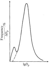
Lognormal distribution of the main peak in the bimodal distribution of oil mist

It should be noted that in the process of drawing frequency distribution curve, the extreme left on the logarithmic scale of the abscissa is not starting at 0 but at the smallest unit of this channel. For example, if the first channel is <0.2 μm, the left side could start at 0.1 μm, which means the value of ΔlgD _p is lg0.2 − lg0.1 = 0.301, not lg0.2 − lg0. In some cases other suitable starting point could be considered according to the situation of the instrument. For another example, when the 3030-type electrostatic aerosol analyzer is used to measure the particle size, the particle size channel represents the nominal diameter, so for the first channel 0.0237 μm which includes the range between 0.0178 and 0.0316 μm, the value of ΔlgD _p is .

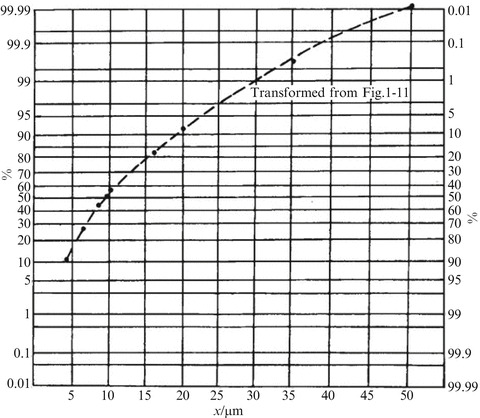
When the points from the curve, which is basically in line with the lognormal distribution, are plotted on lognormal probability graph paper (i.e., normal probability graph paper with the logarithmic scale for the abscissa), a straight line could be obtained although no straight line is got at normal probability graph paper as shown in Fig. 1.19. The straight line (3) in Fig. 1.22 is made from Fig. 1.11 (or Table 1.4). This is a simple method to check whether the particle size distribution fits lognormal distribution. Line (2) in Fig. 1.22 is plotted with the data in Table 1.2. Although the data set distances are unequal, the characteristic of lognormal distribution could also be displayed on lognormal probability graph paper. Since sample number (particle group for number counting) is random, a few deviations from straight line are allowable, but it should not deviate too much. Generally speaking, the middle points should get close to the straight line, while points at two extreme edges (especially big particles for dust) could deviate comparatively more from the straight line, such as the points at the 100 % lower cumulative frequency of line (3) (labeled with Δ for particle size >50 μm) made from Table 1.4 and Fig. 1.19. Although they deviate too much from the straight line, it is still reasonable to consider that the data basically fits lognormal distribution. Because both ends of the scale on lognormal probability graph paper are actually amplified, the error range of cumulative frequency at both 5 and 95 % is four times that of 50 %. In addition, grouping and measurement of both ends are generally coarse, so requirement for points with cumulative frequency smaller than 5 % or larger than 95 % is not so stringent, while it is enough to pay attention to the linear feature between 20 and 80 %.

Fig. 1.22.

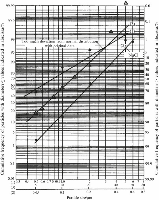
Distribution on lognormal probability graph paper

Experiments have shown that particle size distributions of some dispersed aerosol and aggregated aerosol follow lognormal distribution. From the assumption of the characteristic during solid particle rupture process, particle size distribution was found to approach towards lognormal distribution. Although the reason is heretofore not clear, lognormal distribution has more theoretical meaning than other distribution [8].

If particle size distribution is quite different from normal distribution, such as an extreme case shown in Fig. 1.23 which represents the sampled particle size distribution curve in the cleanroom air, large deviation could be found when the lognormal probability graph paper is plotted. Line 1 on Fig. 1.22 is the resultant line.

Fig. 1.23.

Distribution curve of particle size in the air of a cleanroom

Particle Size Distribution on Log-Log Graph Paper

Experiment has shown that some particle size distribution curves on log-log graph paper are close to be straight and they follow the rule of negative exponent, so they are also termed as negative exponential distribution. For the special case of finer particles, the linear dependence is well presented.

Attenuation Distribution Based on Particle Size

Attenuation distribution gives the information about the change of particle number with the change per unit particle size, which is equivalent with the previous frequency distribution when the ordinate means the particle number per unit particle size spectra instead of the frequency per unit particle size spectra. This is often used in the study of atmospheric aerosol, which will be introduced in 10.1007/978-3-642-39374-7_2 in detail.

Particle Number Cumulative Distributions Based on Particle Size

This means the change characteristic of particle number for the particle size equals with or larger than a certain value. For airborne particles with various diameters in the air of clean environment, their distribution curves of particle size on log-log graph paper are almost parallel straight lines with quite the same slope (especially those particles with diameter larger than 0.1 μm). Figure 1.24 is an example of a cleanroom which is the same cleanroom shown in Fig. 1.23. The feature of the line in Fig. 1.24 is more obvious than that of Fig. 1.23, so it is more useful for practice use. This is used in the classification of cleanness class, which will be illustrated later.

Fig. 1.24.

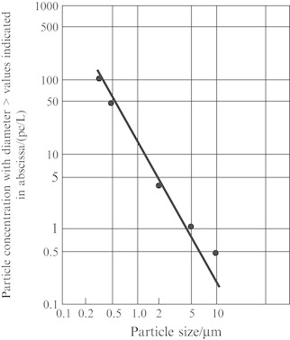
Particle size distribution on log-log graph paper

Atmospheric particles also have this feature, which is usually used in the air cleaning technology. For detailed information, please refer to 10.1007/978-3-642-39374-7_2 about atmospheric particles.

Distribution Based on Density

Particles are not uniformly distributed in terms of density (particle number per unit space or area). For example, when 1 L air is sampled from the cleanroom, the particle number measured by particle counter is 10#. However, particle number is actually not always 10# when 1 L air is sampled. For all that, there is a law existed in the sampled particle number per unit volume of air when particle counter is used.

In general case, the density distribution obeys the law of Poisson distribution. Density data could only be positive integers such as 1, 2, 3, 4, …, instead of continuous one, so density does not follow normal distribution. Since the most important law for discrete data (counting value) is Poisson distribution, particle density distribution should also accord with Poisson distribution. In addition, four conditions are satisfied for the general cleanroom space, which are also required by Poisson distribution:

1. The measured space is much larger than the sample volume, even 10,000 times (the minimum is 100 times)

2. The probability of single particle appearing in the volume of every sample is very small such as several ten thousandths (the minimum is several hundredths)

3. It is incompatible that particle will fall into the sample volume and not.

4. Since particle concentration in the space is quite low, particle number during each sampling process is a small finite value (e.g., less than 10).

The probability of different particle number with Poisson distribution could be expressed as

1.16

where P(ξ = K) means the probability of K particles where K must be positive integer including 0 and λ means the average time of the appearance of incidence, and it also represents the average concentration – average particle number included in the sampling volume.

Figure 1.25 shows the change of Poisson distribution curve when λ increases. The distribution curve for discrete data could only be polygonal line. When λ > 5–10, the curve is more symmetric and close to the normal distribution.

Fig. 1.25.

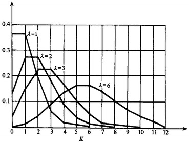
Poisson distribution curve

According to the probability theory, the probability for the appearance of more than K particles could be obtained from Eq. (1.15):

1.17

The probability for the appearance of less than K particles is

1.18

People may be afraid that the unidirectional flow in the cleanroom has almost no dilution effect (please refer to the cleanroom principle in 10.1007/978-3-642-39374-7_8), which will change the distribution law of particle size, so the Poisson distribution may not be applicable. But the Poisson distribution does not require uniform distribution of the particles. For example, during the investigation of flaw spots on the cloth and rejecting rate of piles of mechanical parts, they are both not uniformly distributed. But when enough random sampling time is performed, the conclusion of the law will be roughly in line with the actual situation.

Using the measured data from a cleanroom with unidirectional flow, the above conclusion could be validated.

Table 1.6 shows 440 measured data in a cleanroom with unidirectional flow where the original concentration is comparatively high and the efficiency of air filter is low. The sample volume of each test is 0.1 L. The test shows λ = 1.69.

Table 1.6.

Measured particle number distribution in a cleanroom (with diameter ≥0.5 μm)

	0	1	2	3	4	5	6	7	8	9	10
Measured times	98	125	104	68	28	12	3	1	1*	0	0
Calculated times by Poisson distribution	81.2	137.2	116	65.3	27.6	9.3	2.6	0.6	0.13	0	–

Table 1.6 also lists the data by theoretical distribution with the value of λ. For example, the probability for the appearance of no particle can be calculated

So the times of appearance are 0.1845 × 449 = 81.2. Results show that except for the influence by external interference (data labeled with *), agreement exists between calculation and test. Comparison between them could be clearly seen in Fig. 1.26.

Fig. 1.26.

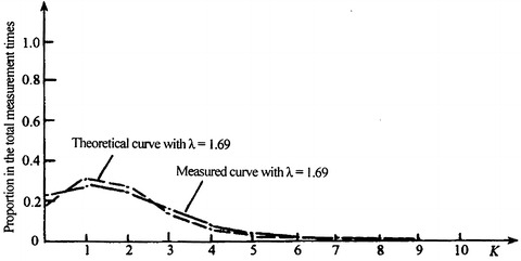
Comparison of curves between test and theory

In the following part, several test examples were performed in cleanrooms with unidirectional flow where the initial cleanness is high. Tests were performed at fixed position. Table 1.7 presents cases in China.

Table 1.7.

Particle number distribution in several Chinese cleanrooms with unidirectional flow and high initial cleanness

Test no.	Test times	Frequency with “0”	Particles with diameter more than 0.5 μm		Percentage with non-“0”	λ #/unit sampling volume L	Probability with “0” (%)	Probability with non-“0” (%)	Frequency equivalent with non-“0”	Ref.
			Frequency with “1”	Frequency with “2”
1	21	18	3	–		0.15	86	14	0.143 × 21 = −3
2	42	41	1	–		0.03	97	3	0.03 × 42 = 1.26	[9]
3	30	28	2	–		0.02	98	2	0.02 × 30 = 0.6
4	20	12	7	1		0.45	63.7	36.3	0.363 × 20 = 7.26
5	20	11	7	2		0.55	57.7	42.3	0.423 × 20 = 8.46	[10]
	20	9	*	*		0.83	43.6	36.4	0.564 × 20 = 11.28

Note: *means there is no information for the current column in original literature, but the value of λ is given. In the fifth case, two times of measurement data in the same cleanroom are provided

Table 1.8 presents some test cases in cleanrooms with unidirectional flow where the initial cleanness is high in China overseas. Test positions are at multiple positions.

Table 1.8.

Particle number distribution in several foreign cleanrooms with unidirectional flow and high initial cleanness

Test no.	Test times	Frequency with “0”	0.12–0.17 μm			Percentage with non-“0” (%)	λ #/unit sampling volume L	Probability with “0” (%)	Probability with non-“0” (%)	Frequency equivalent with non-“0”	Ref.
			Frequency with “1”	Frequency with “2”	Frequency with “3”
1	16	8	4	2	1		0.69#/3 L	50	50	0.5 × 16 = 8	[11]
2	10	9	1	0	0		0.1#/ft3	90	100	0.1 × 10 = 1
3	10	10	0	0	0		0	100	0	0 × 10 = 0	[12]
4	10	8	2	0	0		0.2#/ft3	82	18	0.18 × 10 = 1.8

Data between the examples 2 and 4 from Table 1.8 were collected in three cleanrooms by two particle counters with different types. Both sample flow rates are 0.1 ft³/min (1 ft = 0.3048 m). The resultant conclusions are consistent.

In the measurement examples both in and outside China, except for the calculated value of nonzero time in the third example of Table 1.7, which is quite different from the measured value, others agree well with measurements. This further proves that Poisson distribution is suitable to describe the particle distribution in terms of particle number density.

Poisson distribution is also valid for the problem of studying the particle deposition number on a surface in cleanroom, which also meets the above four conditions. We have applied this conclusion in the study of the relationship between the yield rate and particle number in air, and agreement was found between calculation and experiment [13]. This conclusion will also be useful for the sample of microorganism particles, and detailed information will be introduced later. Statistical analysis of the measurement data of colony in biological cleanroom also support the above conclusion [14], which is shown in Fig. 1.27.

Fig. 1.27.

Comparison between measured data and calculated one by the density distribution of microorganism particles

Concentration Degree of Particle Size Distribution

In a cluster of particles, it will be called monodisperse when particle sizes approach a single value. Its concentration degree is the maximum. On the contrary, it will be called polydisperse when particle sizes are scattering. Its concentration degree is the minimum. However, particle sizes in practice are not likely to be single value, but may be in the narrow range around the two sides of average diameter. Therefore, concentration degree of particles is defined as the percentage between particle numbers corresponding to particles with a certain diameter and the whole particle number.

It is obvious that concentration degree of particle sizes is not an antonym of scattering degree of particle sizes introduced in Sect. 1.3. If small particles with one or two kinds of diameters occupy quite a large number of a particle group, e.g., 90 % of the whole particle number, the scattering degree of this particle group is high, while it does not mean the concentration degree is low. On the contrary, since 90 % of particles have diameter concentrated in a small range, the concentration degree is very high.

It is shown in Fig. 1.16 that the value of standard deviation σ represents the degrees of concentration and scattering of particle sizes. So σ could also be used to stand for the concentration degree or monodispersity of particles. We have such experiences that the absolute error for measuring comparatively large things is normally big, and it is small when tiny thing is measured. σ is only an indication of absolute fluctuation of particle size data. Evaluation of the concentration degree and monodispersity of standard latex particles, the standard particles used for calibrating Royco particle counters, made by American DOW chemical company is a good example, which is illustrated in Table 1.9. Error is related to the absolute value of particle size. In order to avoid the influence, it is more reasonable to use the relative fluctuation value to represent the scattering degree of data. Relative standard deviation, also called change coefficient, is usually used to represent the concentration degree of particle sizes.

1.19

Table 1.9.

Standard of generated particles made by American DOW company (σ of particle sizes)

Standard diameter (μm)	Standard deviation σ
0.365	0.0079
0.557	0.011
0.814	0.0105
0.171	0.013

However, since particle size distribution is usually close to lognormal distribution, it is more reasonable to use lgσ _g instead of σ. σ _g is called geometrical standard deviation.

When the scattering degree of particle sizes is small and suppose they are near from one certain particle size d ₁, we could get the following expression from Table 1.1:

So because .

When is replaced by and the logarithmic coordinate is used, we could get

1.20

We know when , so we can obtain

This is why the following expression is obtained [3]:

1.21

So

1.22

or

1.23

Fuchs (Н.А.Фукс) defined monodisperse particle as those particle group with α ≤ 0.2 (i.e., lgσ _g ≤ 0.087, or σ _g ≤ 1.22) [15]. This means the proportion of particles within the diameter range D ₁ ± 0.2 D ₁ will be 68.3 % where D ₁ is the arithmetic diameter of a particle group and α = 0.2. For example, TSI Co. Ltd from the USA adopts σ _g as the concentration degree of standard particles which were still manufactured by DOW company. They consider standard particles with σ _g < 1.06 as monodisperse particles.

In practice, simplified method could also be used, which uses the proportion of particle numbers within certain diameter range to the whole particle number to represent the concentration degree. For example, if particle number of those with diameter 0.3 μm occupies 70 % of whole number, 70 % represents the concentration degree of these particles. It is obviously shown from the above discussion that although the method to determine the concentration degree is simple, it varies with different size range, so it is preferable to judge based on the value of α.

For modern optical particle counter which will be introduced in 10.1007/978-3-642-39374-7_17, the minimum channel is 0.1 μm, and the largest variation of average diameter in this channel is , which means the ratio between this variation and average diameter is <0.2. The ratio for particles within larger channels will be smaller. Therefore, if we describe the concentration degree with the percentage of particle number in each channel, the ratio will be smaller than 68.3 % mentioned before, and usually it is 60 %. The concentration degree will be higher when it reaches 70–80 %.

Application of Lognormal Distribution

If particle size distribution follows the lognormal distribution characteristic, logarithmic probability graph could be used to determine the concentration degree of particle sizes and various kinds of average diameter.

Determination of Concentration Degree

If particle size distribution curve on the logarithmic probability graph is a straight line, particle size distribution will follow the lognormal distribution, which is shown in Fig. 1.20. Under this condition, Eq. (1.12) could be expressed as

1.24

From Table 1.1 it is known that where D _g is the geometric average diameter. For the case of normal distribution, , so for lognormal distribution, and the above equation could be written as

1.25

This function represents the relative number of particles with diameter D _t. If the total number is 100 %, the percentage of particle number of those with diameter smaller than D _t is

1.26

when

1.27

We know that

Since D _i = 0–D _t when t = −∞ to t, Eq. (1.26) could be written as [16]

1.28

This is the normal distribution N (0,1) and the standard deviation is 1. From Eq. (1.27) we know

1.29

It is obvious that it is easy to solve lgσ _g when t is supposed to be 1 and . Refer to the normal distribution table and Fig. 1.28, the percentage of particle number with diameter ≤D _t when t = 1 is or that of diameter >D _t is .

Fig. 1.28.

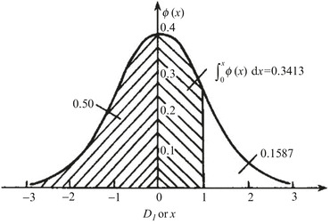
Diagram of normal distribution

Therefore

1.30

In a similar way we could get the following expression for t = −1:

1.31

The value of calculated lgσ _g could be used to determine the concentration degree of particle group and thus to judge if it is monodisperse.

Suppose the actual particle size distribution measured by electronic microscope on monodisperse PSL spherical particles with claimed diameter 0.8 μm is shown in Table 1.10.

Table 1.10.

Distribution of 0.8 μm PSL particles

Interval (μm)	Cumulative distribution (%)
≤0.6	1.2
≤0.7	6.1
≤0.8	65.5
≤0.9	88.0
≤1.0	98.5
≤1.2	100.0

Data of Table 1.10 plotted on Fig. 1.29 is a straight line A. We could obtain

Fig. 1.29.

Calculation of σ _g from lognormal distribution probability paper

Therefore it is reasonable to consider this particle group as monodisperse, and 68.3 % of particle diameter will be in the range of 0.784 ± 0.108 × 0.784 = 0.784 ± 0.085 μm.

Calculation of Average Diameter

As mentioned before, it is quite difficult to calculate the average diameter. But for the case of lognormal distribution, data could be plotted on the lognormal distribution probability graph, and then it is easy to calculate the median diameter D ₅₀, geometrical standard deviation σ _g, and various average diameters. Here only the results of various average diameters calculated are shown [16]. Process of data plotting could be referred to Fig. 1.29.

The calculation expressions between various average diameters and D ₅₀ are presented below:

Geometric mean diameter

1.32

Arithmetic mean diameter

1.33

Specific length diameter

1.34

Specific area diameter

1.35

Specific mass diameter

1.36

Area weighted diameter

1.37

Volume weighted diameter

1.38

Various average diameters of the example line (2) on Fig. 1.22 are calculated, which is shown in Fig. 1.29. Since the diameter is , which corresponds to 83.13 % on the accumulative distribution curve for geometric average diameter , the geometric standard deviation is

The above results are close to the calculated results from the data of Table 1.2. The more the linear proportionality on the lognormal probability graph is, the less difference between them it becomes.

Relationship Between Particle Size Distributions

The abovementioned particle size distribution represents the particle number distribution corresponding to the particle size. For particle mass distribution on particle size, it represents the percentage of particle mass corresponding to certain particle size in the whole mass. For particle area distribution on particle size, it represents the percentage of particle area corresponding to certain particle size in the whole area. They can be derived from the particle size distribution, and measurement on mass or area is not needed. Since each weighted distribution of lognormal distribution is also lognormal, they are parallel straight lines with the same σ _g. Their relationships are

1.39

1.40

where

• is the particle size at 50 % in the mass distribution curve, i.e., the mass median diameter; when lognormal distribution is valid, it is called the mass geometric average diameter;

• is the particle size at 50 % in the area distribution curve, i.e., the area median diameter; when lognormal distribution is valid, it is called the area geometric average diameter.

From the example of Fig. 1.29, we could know and from calculation, and straight lines which represent area distribution and mass distribution and which are parallel to the particle number distribution could be plotted. It should be noted that in order to fit the scale on probability graph paper well, only data group of those “<0.6” is needed at one edge, while those between 0.6 and 1.0 could be considered as data of “≥0.6,” which means the proportion of data <0.6 is 98.4 % while that of ≥0.6 is 1.6 %. If more precise data are needed, subdivision of two edges could be made.

As for the case of surface contamination, area distribution is preferred; while for the hygiene problem, mass distribution is used, where mass of particles have direct implications for the problem. When we are dealing with the problem in the cleanroom, particle number distribution with particle size is used.

Statistic Parameter of Particle Number

Statistic calculation of particle size is needed for the abovementioned particle distributions. It is a basic statistic problem that how many particles should be sampled in the particle group of each sample so that the error of the measured particle size is minimized.

From the principle of statistics, standard deviation of average value equals with the ratio of standard deviation σ to the root of sample number, which is shown in Eq. (1.41):

1.41

where n is the particle number.

The real size of particle under the 95 % confidence level is

1.42

where is the relative error of particle size. When it is set to be ΔC, the following requirement should be met:

So we could get

1.43

The above expression was used in Ref. [17] to obtain the necessary particle number for counting of monodisperse standard particles. According to the definition of monodisperse aerosol, we know

For calibration of particle counter, the requirement is much stricter, so it could be assumed ≤3 %. With the above data, Eq. (1.43) becomes

During the counting process, the abovementioned problem of relative error exists. When particle number is too less, man-made error will exist because of inadequate randomness. When it is too much, the workload of counting process is heavy. When particle counter is used, to count 178 particles is not difficult, so 300–500 standard PSL particles are needed for calibrating particle counter in the national standard “calibration method of the performance of particle counter,” which will result in error smaller than 3 %.

For polydisperse aerosol, σ is unknown, so is . But for common aerosol particles, the value of σ could be assumed. Now we assume σ in Table 1.2 is 0.13 (in fact it is 0.1287), then we could obtain

For the usual test, the relative error of 5 % is acceptable. Therefore the particle counting in Table 1.2 should be

Now we know from the table that , which meets the requirement.

Moreover, Ref. [18] presents the guideline to measure the particle number needed. Since it is generally introduced, we will not introduce in the book. For those readers who need the information, please find the original paper.

References

- 1.Ma GD, Hao JM . Air pollution control engineering. 2. Beijing: China Environmental Science Press; 2003. [Google Scholar]
- 2.Lin ZH . Sampling technique and measurement of dispersity of NaCl aerosol. Beijing: Tsinghua University; 1983. [Google Scholar]
- 3.JACA Guideline for the generation method of aerosol for pollution control. J Jpn Air Clean Assoc. 1994;32(2):60–83. [Google Scholar]
- 4.Hinds WC (1989) Aerosol technology (trans: Sun Yufeng, Chapter 4). Heilongjiang Science and Technology Press, Harbin (In Chinese)
- 5.Yan HL, Wu HP, Zhang JK (1983) Analysis of the relationship between the average size and the polarizing fault of oil mist aerosol and its dispersity. Institute of HVAC at China Academy of Building Research, People’s Liberation Army No. 57605 of the People’s Republic of China (In Chinese)
- 6.Zhao RY, Qian BN, Xu WQ . Characteristic of aerosol generator with Cold DOP aerosol. Beijing: Tsinghua University; 1987. [Google Scholar]
- 7.Wang JS, Zhu PK, Zhou GH et al (1983) Technical report for the development of JL leakage detection apparatus. Institute of HAVC at China Academy of Building Research, Liaoning Hongbo Radio Factory (In Chinese)
- 8.Fuchs HA (1960) The mechanics of aerosols (trans: Gu Zhenchao). Science Press, Beijing (In Chinese)
- 9.Xu ZL, Gu WZ Calculation of the minimum sampling volume for particle counter in environments with different air cleanliness levels. J HVAC. 1980;1:22–25. [Google Scholar]
- 10.Yang YD (1987) Discussion of the deviation phenomena of statistical average value of particle number during measurement. In: Proceedings of the academic conference on air cleaning measurement techniques, Institute of Scientific and Technical Information at Hebei University of Technology (In Chinese)
- 11.Kamishima K Performance of ULPA filter in ultra cleanroom. Jpn Air Cond Heat Refrig News. 1984;24(1):163–172. [Google Scholar]
- 12.James B (1989) Acceptance inspection of cleanroom with Class 1 (trans: Du Chunlin, Proofread by Chen Changyong). Compiler group for code for construction and acceptance of cleanroom, pp 303–304 (In Chinese)
- 13.Xu ZL Relationship between the yield and the air cleanliness level in the clean environment. Mech Eng. 1981;3(1):45–49. [Google Scholar]
- 14.Yao GL . Discussion of the bacterial deposition method to measure the air cleanliness level in cleanroom. Shanghai: Tongji University; 1981. [Google Scholar]
- 15.Sano I Generation of smoke. J Jpn Air Clean Assoc. 1971;9(5):2–11. [Google Scholar]
- 16.Sato E Introduction to aerosol technology. Build Equip Water Heat Construct. 1971;9(8):47–63. [Google Scholar]
- 17.Specification description of “Methods for testing the performance of airborne particle counter” (1983) Institute of HVAC at China Academy of Building Research (In Chinese)
- 18.Richard D (1981) Aerosol handbook (trans: Zhou Jinqin). Atomic Energy Press, Beijing, pp 131–132 (In Chinese)