Filtration Mechanism of Fine Particle

Abstract

There are usually four kinds of methods available to separate solids or liquid particles from an aerosol:

There are usually four kinds of methods available to separate solids or liquid particles from an aerosol:

1. Mechanical type – gravity dust collector, impinger, and cyclone

2. Electrostatic force – single-stage electrostatic precipitator, double-stage electrostatic precipitator, etc.

3. Washing – spray scrubber, water film precipitator, Venturi dust collector, etc.

4. Filtration – filling-in filter, bag filter, etc.

In the field of air cleaning, the particle concentration is typically very low compared with industrial dust separation applications, and the particle size is small. Hence the reliability of the performance of filters must be assured. Therefore, filtration and separation techniques are often used to remove particles in the airstream and are the focus of this chapter.

Filtration and Separation

Air filters remove particulate matter via several mechanisms including interception, impaction, and diffusion. According to the position of the capture particles, particulate air filters may be divided into two types: (1) surface filter and (2) depth filter.

Surface filters have many forms including metal wire mesh and perforated plate, where particles are captured on the surface. Chemical porous membrane is made from fibrous ester (nitrocellulose or cellulose acetate), which looks like a piece of white paper, and its characteristic follows that of a surface filter. The thickness of this kind of membrane filtration medium is approximately 50 μm. Circular pores with diameter 0.1–10 μm are uniformly distributed on it; the pore size is controlled during the membrane manufacture process. The average number of pores is about 10⁷–10⁸ #/cm², and the porosity can be as high as 70–80 %. For theoretical purposes the pores are often treated as capillaries. Particles larger than the pore diameter are captured on the surface and the filtration efficiency could be 100 %. It is believed that the minimum size of particles captured by the membrane could be 1/10 to 1/15 of average pore diameter. Figure 3.1 shows the structure of a surface air filter and the schematic of particle capture.

Fig. 3.1.

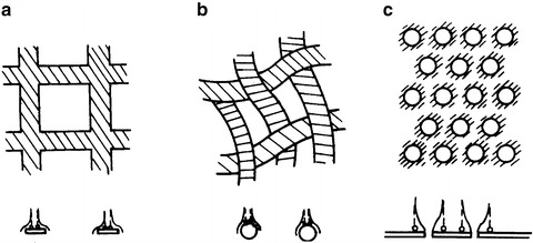
Surface air filters (a) Single ribbon model (plate); (b) Isolated cylinder model (metal wire mesh); (c) Small pore model (perforated plate)

Depth filters can be divided into two with high and low solid fractions (also called low porosity and high porosity). Particles are captured on the surface or inside the medium layer.

The solid fraction α can be expressed as:

Depth filters with a high solid fraction (α > 0.2) have various forms, such as granular filling layer (gravel layer, activated carbon layer, etc.), porous filter media and thick filter paper. Their structure and a schematic of the particle capture process are shown in Fig. 3.2.

Fig. 3.2.

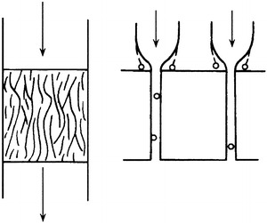
Depth filter with high solid fraction (capillary model)

Depth filters with low solid fraction (α < 0.2) occur as fibrous filters, high-efficiency air filters with a thin paper medium and foamed material filter, etc. Their structure, together with a schematic of particle capture process, is illustrated in Fig. 3.3.

Fig. 3.3.

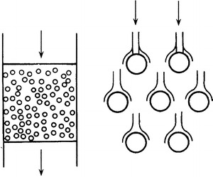
Depth filter with low solid fraction (isolated cylinder model)

Although the particle capture mechanism of a surface filter is simple, most of these filters have low efficiency and so are of little practical use. On the contrary, microporous membranes have an extremely high efficiency. With the exception of liquid filtration, they are mainly used for sampling and the final filter for dust-free and aseptic systems where the cleanliness requirement is very high. Moreover, they are more reliable than fibrous filters.

Depth filters, with high solid fraction, have a very complex internal capillary structure, and thus the particle capture mechanism is extremely complex. To date few have performed a theoretical study.

Depth filters, with a low solid fraction, such as fibrous filter (including fiber-filled layer filter, nonwoven filter, and HEPA filters), also have a complex internal fiber distribution. However, since the porosity is large (shown in Figs. 3.4, 3.5, and 3.6), the interspace is smaller than what is shown in these figures when hundreds of fibrous layers overlap each other. In order to simplify the study, a single fiber of a filter layer is often treated in isolation. The pressure drop of this type of filter is not high, but its efficiency is high, and so has practical significance, especially in the field of air cleaning technology. For investigating the filtration mechanism, a much deeper theory and experimental verification is required. This chapter introduces the particle filtration mechanisms for fibrous filters, while the next chapter will discuss the particle capture mechanism of the electrostatic precipitator.

Fig. 3.4.

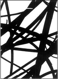
Structure of domestic-made glass fiber filter (η = 99.99999 % with amplification ratio 10,000)

Fig. 3.5.

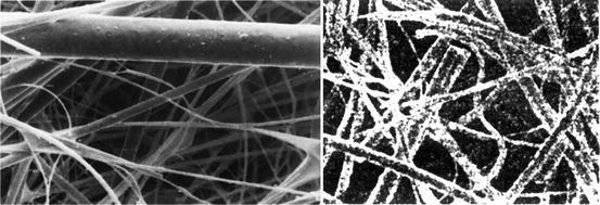
Stereo of fibers from foreign air filter paper made by glass fiber [1, 2]

Fig. 3.6.

Structure of foreign fibrous media [3] (a) glass fiber ρ = 2.55 g/cm³; (b) nylon ρ = 1.14 g/cm³; (c) polypropylene ρ = 0.97 g/cm³; (d) Tacryl fiber ρ = 1.17 g/cm³; (e) esterified fiber ρ = 1.38 g/cm³; (f) chlorinated alvar ρ = 1.39 g/cm³; (g) cotton fiber ρ = 1.54 g/cm³; (h) vinylon ρ = 1.3 g/cm³; (i) cellulose acetate ρ = 1.32 g/cm³

Fundamental Filtration Process of Air Filters

The characteristic of captured particle and filter material, as well as their interactions, has extremely important influence on the filtration process. Most researchers are inclined to formulate the filtration process as two stages.

The first stage is called the steady stage, where particle capture efficiency and pressure drop of air filters do not change with time; instead they are determined by the intrinsic geometry of filters, property of particles, and feature of airstream. In this stage, the change of filter thickness is small because of particle deposition. For the case of airstream with low concentration of particles such as indoor air filtration in air cleaning technology, this stage is important for air filters.

The second stage is called nonsteady stage, where the particle capture efficiency and pressure drop change with time and they depend not only on particle property but also on the influence of particle deposition, gas erosion, water vapor, etc. Although this stage is longer than that of the first stage, and it has the decisive significance to the general industrial filters, to some extend it is only meaningful to the filters with efficiency lower than sub-HEPA filters in air cleaning technology, and it is not meaningful to filters with efficiency equal with and higher than sub-HEPA filters.

Filtration Mechanism of Fibrous Air Filters

It is already known that there are at least five kinds of mechanism, instead of one mechanism, that play roles in the particle capture process during the first stage of air filtration for fibrous filters.

Interception (or Contact/Hook) Effect

Inside the fibrous layer, fibers are located randomly and form numerous meshes. When particles with certain size approach fiber surface when following the streamline, suppose the distance between the streamline (also the centerline of particle) and fiber surface is equal to or smaller than particle radius (shown in Fig. 3.7, r ₁ ≤ r _f + r _p), particles will be intercepted and then deposited on the fiber surface, which is called interception effect. Sieve effect also belongs to the interception effect (shown in Fig. 3.8), and sometimes the interception effect is called filtration effect.

Fig. 3.7.

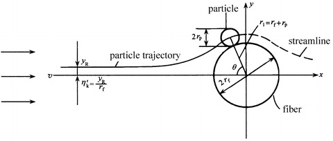
Schematic of interception effect

Fig. 3.8.

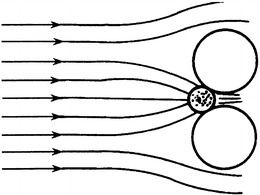
Schematic of sieve effect or filtration effect as one of interception effects

However, interception effect or sieve effect is not the only one or main effect in particle filtration of fibrous filters, so fibrous filters could not be considered as a sieve. Sieve only removes particles whose diameter is larger than the hole, while for fibrous air filters, not all the particles whose diameter is smaller than mesh size could penetrate, and the most penetrating particle size is located in some range. Particles are not all removed by the surface of fiber layer – deposition. Otherwise, the pressure drop of air filters will increase rapidly when the mesh holes are blocked by particles, which is not true. In fibrous filters, particles will go deeply through fibrous layers, so there are other mechanisms for particle capture process.

Inertial Effect

Because of the complex arrangement of fibers, streamline will change directions frequently and abruptly when air flows through fibrous layers. When the particle mass is large or its velocity (which could be approximated by air velocity) is large, by virtue of its inertia, particle will not follow the streamline when air flows around fibers. Therefore, particles will deviate from the streamline when approaching fibers, then collide with fibers and deposit on it (shown in Fig. 3.9, position A).

Fig. 3.9.

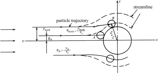
Inertial effect (A) and inertial interception effect (B)

Diffusion Effect

It is much obvious for small particles that show Brownian motion caused by the collision between gas molecules and particles. At normal temperature, the diffusion distance could be 17 μm/s for 0.1 μm particles, which is several times or even dozens of interspace distance between fibers. This results in the larger possibility of particle deposition onto fiber surface (as position A shown in Fig. 3.10). However, the Brownian effect is weaker for particles with diameter larger than 0.3 μm. In this case, particles will not deviate from the streamline and deposit onto fiber surface only by this effect.

Fig. 3.10.

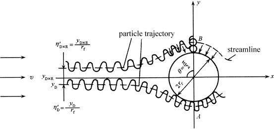
Diffusion effect (A) and diffusion interception effect (B)

Gravitational Effect

Particles will deviate from the streamline under the influence of gravity when they pass through fibrous layers, which means they will deposit on fiber surface by gravitational deposition (shown in Figs. 3.11 and 3.12). The time usage for airflows through fibrous air filters, especially paper filters, is far less than 1 s, so particles with diameter smaller than 0.5 μm will pass through fibrous layers without deposition on fiber surfaces. Therefore, it is reasonable to ignore the effect of gravitational deposition.

Fig. 3.11.

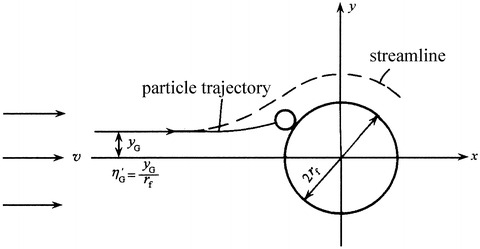
Gravitational effect (gravity is parallel to airstream)

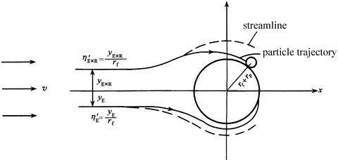
Fig. 3.12.

Gravitational interception effect (gravity is perpendicular with airstream)

Electrostatic Effect

By various reasons, charge may exist on both fibers and particles, which will cause electrostatic effect and attract particles (shown in Fig. 3.13). Except for the case of intentional charge on fibers or particles, both fiber charges by friction during the manufacture process and particle charge by charge induction will not exist for a long time. The induced electric field is very weak, and the resulting attractive force is very small. So this kind of electrostatic effect can be neglected.

Fig. 3.13.

Electrostatic effect and electrostatic interception effect

For the process of particle capture in fibrous filters, all the mechanism or maybe one or some mechanism will take effect, which depends on the particle size, density, fiber thickness, solid fraction, and air velocity.

Procedures to Calculate Efficiency of Fibrous Air Filters

Although the abovementioned effects exist in the process of particle capture inside the fibrous air filters, it is quite difficult to make description using refined mathematical expressions. Semiempirical formula is obtained based on the reliable experimental data and simplified model. Results from these formulas do not match the experiment completely. So the purpose of performing calculation is to make analysis and comparison qualitatively, not to obtain the accurate data.

For the calculation of fibrous filters with low solid fraction, the theoretical basis is still the isolated cylinder method, which was put forward by Langmuir and had the following assumptions:

1. Filters are made of uniformly distributed isolated circular fibers with the same material.

2. Fibers are perpendicular to the airflow, and they are far enough from each other.

3. Particles are spherical.

4. Filter surface is clean, so only the efficiency of the first stage is considered.

5. Particles attached to the fiber surface will not resuspend.

Based on the theory of isolated fiber, Fuchs et al. developed it theoretically [5]. In the field of HEPA filter, Iinoya et al. performed experimental study. Based on these researches, the following procedures calculate the efficiency of fibrous filters:

1. Determine the main mechanisms among these five effects according to the particle characteristic, filter performance, and condition (usually only the effects of interception, inertia, and diffusion are considered).

2. Determine the individual efficiency η′ of corresponding mechanism for isolated single fiber.

3. Determine the total efficiency η _Σ of the combined mechanisms for isolated single fiber.

4. Determine the total efficiency η _Σ of the combined mechanisms for single fiber (not isolated) inside the filter, when the interference influence of adjacent fibers is considered.

5. Determine the total efficiency η of filter from the value of η _Σ according to the lognormal penetration law.

Particle Capture Efficiency of Isolated Single Fiber: Isolated Cylinder Method

Interception Efficiency

Figure 3.7 illustrates that interception is caused by geometrical effect, which means the particle’s capture by direct interception or contact. Since fiber is considered as circular cylinder (as shown in Fig. 3.6, fibers inside glass fibrous filters are regularly circular cylinders), particles will be captured onto these fibers which face towards the incoming airflow stream and all the particles within the airstream with the width d _f (fiber diameter) shown in part (a) of Fig. 3.14. When all these particles are captured, the efficiency is 100 %. But before arriving at the fiber surface, air will flow around the fiber. So particles in the range between y = r _f and y ₁ = r _p + r _f are likely to be captured which is shown in part (b) of Fig. 3.14. Here r _p and r _f represent the particle radius and fiber radius, respectively. And y means the distance between any position inside the flow and the cylinder axis.

Fig. 3.14.

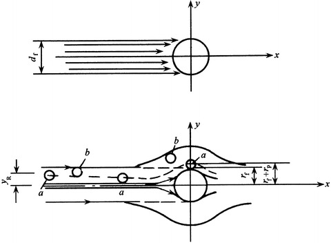
Particle range by interception capture

The width of the airflow is r _p, which is smaller than the width of the previous flow that fiber faces. So the interception efficiency is a probability with the value less than 1, and it equals with the ratio between the particle number per unit time in the range of r _p for a fiber with unit length and the total particle number that flows towards the fiber. When it is assumed uniform for particle concentration, it also equals with the flow rate ratio.

For a fiber with unit length, the flow rate that passes through the fiber is r _f v, the multiplication of fiber radius and air velocity at the far distance. All the captured particles are within the flow between r _f and r _f + r _p. The corresponding flow rate can be expressed as

3.1

Since , it could also be rewritten as

3.2

where y _R is the distance between the fiber axis and the effective particle trajectory at the infinite, where particles within this range can be captured due to the interception effect at infinite distance. In practice, the distance far enough is considered as the situation at infinite.

W _R is the flow rate within the width of y _R.

Therefore the particle capture efficiency under certain effect is defined as the ratio between the width of the effective particle trajectory for particle capture and fiber radius.

In fluid dynamics, the velocity distribution around the circular cylinder for the common viscous flow and Re < 1 is expressed as [4]:

where

• v _y and v _θ are radial velocity and tangential velocity near the cylinder, respectively;

• v is the velocity at infinite for θ = 0 or θ = π;

• θ is the angle between radius and horizontal axis;

• Re is the particle Reynolds number.

Attention should be paid to the definition of Re number. In the study of air flow, the flow Reynolds number is applied. While in the study of particles, the particle Reynolds number should be used:

where both the density ρ and air viscous coefficient μ are used for gas and v and d are determined according to the study object. For the airflow, v is the air velocity, and d is the characteristic size. In the study of airflow inside the pipeline, d is the pipe diameter. For the particles, v is the relative velocity between particles and air, which is the settling velocity of particles, and d is the particle diameter. For the airflow, it is laminar flow for Re < 2,000 and turbulent flow for Re > 4,000. For the particles, the flow around the particle is laminar for Re ≤ 1, while vortex appears downstream of particles for Re ≥ 2. The number and strength of vertex increase with the increase of Re, which means particles are gradually surrounded by turbulent flow.

The tangential velocity at θ = π/2 is:

Therefore

3.3

The expression shows that the interception efficiency is a function of Re and R = r _p/r _f. R is the interception parameter, and it is used to describe the sedimentation effect under the effect of interception mechanism.

Furthermore, Norio and Iinoya [7] obtained the approximate expression for the velocity distribution inside the boundary layer near cylinder as follows:

3.4

Inertial Efficiency

Based on the similar definition of Eq. (3.2) and Fig. 3.7, the inertial efficiency could be expressed as follows for the extreme trajectory case:

3.5

where W _St is the flow rate in the width of inertial capture. It is related to the inertial force on the particle and velocity distribution, not only the thickness of the layer r _p. So movement equations must be solved. Given the resistance of airflow, equations could be written for small Re number (usually it is smaller than 1) and curvature movement of particles as follows:

3.6

where

• u _x and u _y are x- and y-component of particle velocity, respectively;

• v _x and v _y are x- and y-component of air velocity, respectively;

• F _x and F _y are x- and y-component of external force, respectively;

• μ is the viscous coefficient of air.

But it is difficult to solve this nonlinear partial equation. It is common to use approximation method or semiempirical expression. They have the following form:

Since later calculation will not use , the exact data will not be cited here. We emphasize on the parameter St:

3.7

where

• ρ _P is the particle density, kg/m³;

• μ is the viscous coefficient of air, Pa · s;

• c is the slip correction factor of particle, shown in 10.1007/978-3-642-39374-7_6.

St is dimensionless and it is termed as inertial parameter or Stokes parameter. It represents the ratio of inertial force and air resistance. When St → 0, inertial force disappears and particle velocity becomes consistent with air velocity. When St reaches a small value or a critical value, inertial force on particles cannot offset the attractive force from the airflow; it cannot settle onto the fiber surface. Suppose the value of St is less than 0.1, inertial efficiency is very small. Inertial efficiency increases with the increase of St number, which corresponds with the increase of air velocity, particle size, and density, as well as the decrease of fiber size.

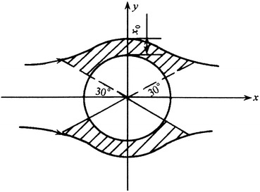
Diffusion Efficiency

Randomized movement of highly dispersed particles makes free displacement in all directions. When an isolated cylinder or fiber is placed in this kind of particle-laden flow, particles will be excluded from the adjacent airflow layer and then deposited onto its surface. The angle range is about 30° ≤ θ ≤ 150°, which is shown in Fig. 3.15.

Fig. 3.15.

Range of particle diffusion deposition

Suppose the thickness of diffusion layer is x ₀ at θ = π/2, which is equivalent to the range between r _f and r _f + r _p for interception effect, Langmuir obtained the following expression:

3.8

where D is the air diffusion coefficient.

Based on the similar definition of Eq. (3.2), diffusion efficiency expression could be derived with Eq. (3.3), because it is mainly dependent on the pure geometrical factor: diffusion layer thickness. We obtain the following expression:

3.9

So the expression for diffusion efficiency is obtained by inserting Eq. (3.8) into Eq. (3.9).

In addition, the particle-laden flow rate towards the circular cylinder with unit length is πd _f k, where k is the mass transfer coefficient, m/s. So the following expression is obtained based on the similar definition of Eq. (3.2):

3.10

where Sh is the Sherwood number (), Sc is the Schmidt number (), and Pe is Peclet number ().

Gravitational Efficiency

Efficiency caused by gravitational settling could be written as:

3.11

where v _s is the settling velocity and v is the air velocity.

According to the study performed by Fuchs, additional item related to R should be added to the equation.

When airflow is perpendicular to the fiber surface and goes downwards, it is:

3.12

When airflow is perpendicular to the fiber surface and goes upwards, it is:

3.13

When air flows parallel to the fiber surface, it is:

3.14

Electrostatic Efficiency

Expressions for three conditions are presented directly [9].

1. Both fiber and particles are charged:

   3.15

   where Q is the charge on fiber with unit length and q is the charge on particle.
2. Fiber is charged, while particles are not:

   3.16

   where ε is the dielectric constant.
3. Fiber is not charged, while particles are:

   3.17

Dimensional constants in the above three equations should have the same unit with the electrostatic charge.

Total Efficiency of Isolated Single Fiber

As mentioned before, gravitational and electrostatic effects could be omitted in the usual case, so the main particle capture mechanisms for fibrous filter include interception, inertial, and diffusion effects. If one mechanism works while others do not, the total efficiency of isolated single fiber with unit length equals with the summation of these three individual efficiencies, i.e.,

3.18

However, in fact these mechanisms take effect simultaneously. It is shown in Fig. 3.7 that under the inertial effect only, particles will not be captured when they do not touch fibers; however, it will still be captured by interception effect when the centerline trajectory arrives r _p away from fiber surface. This is called inertial interception effect. This means that the distance between the axis and the trajectory for particle capture at far distance is not y _R for interception effect only, nor y _St for inertial effect only, but the enlarged distance y _St,R for both effects. For the case of small Re flow (smaller than 1), Davies put forward the following expression [10]:

3.19

where parameters St and R are included, which means this efficiency is related to both inertial and interception effects.

Furthermore, the curve obtained from computer simulation by Susumu can be used for calculation, which is shown in Fig. 3.16 [8]. Naoya also obtained similar result [11].

Fig. 3.16.

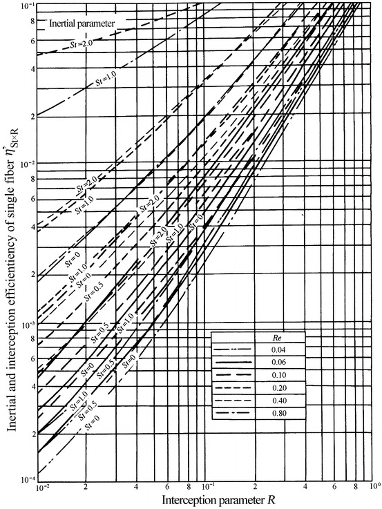
Inertial interception efficiency

It is also shown in Fig. 3.10 that although particles do not arrive at the fiber surface with the diffusion effect only, when it is at r _p away from the surface, it will also be captured by interception effect. This is termed as diffusional interception effect. This means that the distance between the axis and the trajectory for particle capture at far distance is not y _R for interception effect only, nor y _D for diffusion effect only, but the enlarged distance y _D,R for both effects. According to the same definition of Eqs. (3.2) and (3.10) is derived:

3.20

So the total efficiency for isolated single fiber is expressed as:

3.21

Particle Capture Efficiency of Single Fiber Inside Filter: Influence of Fiber Interference and Correction Method

Mechanism of particle capture for isolated single fiber has been introduced earlier. But the situation inside fiber (fiber filling layer or filter paper) is more complex, because the space distribution of fiber, fiber density, and combination form of fibers are different, and the velocity field around fiber is different from that of isolated fiber. Correction of fiber interference to the efficiency of single fiber is needed. Since the interference effect becomes larger with the increase of solid fraction inside the filter, solid fraction α is included in the correction factor. Three kinds of correction method will be illustrated in the following chapter.

Effective Radius Method

This method was proposed by Davies for small Re flow (Re < 1) [4]. Based on Eq. (3.19), the efficiency expression for three simultaneous effects can be written as:

3.22

Compared with Eq. (3.19), it has addition item related to 2/Pe, where Peclet number Pe is a function of diffusion coefficient D and its reciprocal is called as diffusion parameter and labeled as De. This establishes relationship between and three effects.

Given the interference influence of adjacent fiber, the concept of effective fiber method is adopted, and the correction factor including fiber solid fraction α is introduced. The total efficiency of single fiber with unit length is obtained:

3.23

When α < 0.02, real average radius is used for the fiber radius in each parameter. When α > 0.02, effective radius r _fα is used to replace real average radius. The value of effective radius could be obtained by the experimental data ΔP _α:

3.24

where H is the thickness of filter layer, m; v is the filtration velocity, m/s; μ is the air viscous coefficient, Pa · s; and ΔP _α is the experimental data of filter pressure drop, Pa.

Nonuniform Coefficient Method of Structure

This method was proposed by Fuchs [12], which presented the efficiency expression under various effects for single fiber inside filters:

3.25

3.26

3.27

3.28

3.29

where

• I is the parameter for combining the influence of interception with inertial effect;

• Ku is the Kuwabara hydrodynamic factor.

Total efficiency of single fiber is expressed as:

3.30

where both Ku and ε are parameters when the influence of fiber interference is considered.

3.31

3.32

where ε is also called nonuniform coefficient of structure, which represents the ratio of the force acting on fiber with unit length inside the ideal filter to that of real filter.

F _B is determined by theoretical equation, i.e.,

3.33

F _F is determined by experimental data of filter pressure drop ΔP _α, i.e.,

3.34

Both F _B and F _F are dimensionless.

Except for the above correction of filter interference, Fuchs also introduced the slip factor on fiber surface when the fiber size is very small and close to the mean free path of air λ. Since this influence is usually very small, it will not be explained in detail.

This is a complex method for calculation, but it fits well with experiment, which is shown in Fig. 3.17.

Fig. 3.17.

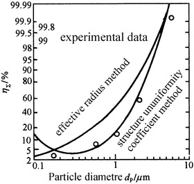
Comparison between calculation and experiment for η _Σ

Experimental Coefficient Method

Chen established the relationship between the efficiency of single fiber inside filter under the fiber interference effect and the efficiency of isolated single fiber [13], i.e.,

3.35

where is calculated by Eq. (3.21). Because this equation is simple and easy for calculation, and it has been validated by experiment, it is frequently used in the literature at present.

Semiempirical Equation Method

This method was proposed by Iinoya in 1970 [6], which assumed that paper filter was made by compression on fibrous filter along the width direction. With the method for fibrous filter, data were processed by single fiber efficiency when both diffusion and interception effects were dominant while inertial efficiency was omitted. In the experiment, fiber diameter ranges from 0.92 to 17.7 μm, and solid fraction α is between 0.091 and 0.292. Semiempirical expression for the efficiency of isolated single fiber was obtained:

3.36

where A ₀ is the theoretical stream function around single fiber when no interference effect was considered.

3.37

At last, the total efficiency of single fiber inside filter was derived:

3.38

Using this method, we could get the monotonic relationship between the increased efficiency and the decreased particle size. However, it cannot reflect the particle size corresponding with the minimum efficiency.

Logarithmic Penetration Expression for Calculation of Total Efficiency of Fibrous Filter

Logarithmic Penetration Expression

After calculation of single fiber efficiency inside fibrous filter, logarithmic penetration expression is applied to obtain the efficiency of whole filter η.

Take a look at the filtration layer in Fig. 3.18 at first.

Fig. 3.18.

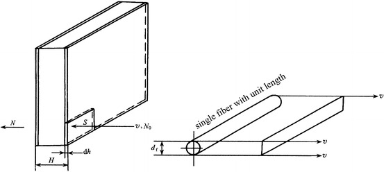
Unit volume inside filter for particle capture

Suppose diameters of fibers inside this layer are the same, and all fibers are perpendicular to the airflow. When the initial concentration is N ₀ and filtration velocity is v, and concentration after filtration becomes N, then the change or decrease of concentration passing through the filtration layer equals with the number of particles captured inside the filtration layer.

Now let’s study the case of unit volume, whose layer has area S and thickness dh. If the change of concentration is dN when air goes through the layer vS in unit time, the number of particles captured is −vSdN.

As mentioned before, the filtration efficiency of single fiber with unit length is η _Σ, so with the efficiency definition in Eq. (3.1), the number of particles captured by fiber with unit length per unit time is η _Σ d _f v′N, where v′ is the average velocity across spaces between fibers, i.e.,

3.39

d _f v′ represents the volumetric flow rate across fibers.

After air flows across this layer vS, the particle concentration decreases by –vSdN. For air with particulate concentration N passing through this layer which contains the total length of fibers L, the number of particles captured is η _Σ d _f v′NL. These two data should be equal, i.e.,

where L is the total length of fibers inside the unit layer, i.e.,

3.40

After integration, we get:

3.41

At the position H = 0, all the particles will penetrate, i.e., N = N ₀.

Replacing the expression of C into Eq. (3.41), we get:

3.42

We denote K′ = N/N ₀, and insert it into Eq. (3.42). When the above equation is transformed into logarithmic function (lg x = 0.434 lnx), we get:

3.43

K′ is expressed in decimal. If we denote K = K′ × 100 % and it is called penetration of filter, the above equation becomes:

3.44

When K is obtained, we get:

For example, lg K = 0.95, then we get K = 8.9 % and . When the exponential function is used, Eq. (3.42) becomes:

3.45

Equation (3.44) is called logarithmic penetration expression of filter, which is the fundamental law in the study of filter efficiency [4].

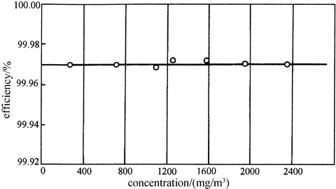
It is shown from Eq. (3.42) that is constant. It does not change with the variation of initial concentration N ₀. So efficiency of filter will not vary with initial concentration in the airflow. Figure 3.19 is the experimental result of oil mist method for the relationship between efficiency and initial concentration, which is performed by Architectural Research Institute of former Ministry of Metallurgical Industry. The result is consistent with that of logarithmic penetration theory. But recently, results using particle counting method on filters show that change of efficiency at 0.1肼μm synchronized with initial concentration [14]. When the latter changes by an order of magnitude, the former changes by about an order of magnitude. At present no explanation has been made for this result.

Fig. 3.19.

Relationship between penetration and initial concentration

In this equation, . According to Zhou Bin’s analysis [15], there is another kind of expression . And the difference between them is given. It should be also noted here that the case with α = 1 cannot be explained with the latter expression, because the unreasonable result will be obtained.

Recently results using particle counting method on filters show that change of efficiency at 0.1 μm synchronized with initial concentration [14]. When the latter changes an order of magnitude, the former changes by about an order of magnitude. At present no explanation has been made for this result.

In fact, values of K′, H, α, and d _f are usually determined by experiment. Then the total efficiency of single fiber with unit length is derived by Eq. (3.43):

3.46

Then the relationship among , , and α is established. The third parameter is calculated when two others are known. This is the common procedure to study the filtration mechanism of fibrous filter.

Applicability of Logarithmic Penetration Expression

Filtration layer or fibrous filter consists of multilayers of fiber net. During the derivation process of logarithmic penetration expression, the following conditions must be met:

1. Fibers arrangement is regular.

2. The probability of particle capture for each fibrous layer is the same.

3. No resuspension phenomena occur for particles captured on the fiber surface.

In this way, a linear relationship among penetration, thickness H, and solid fraction α is established, because the item (1 − α) from Eq. (3.42) to Eq. (3.46) is close to 1 for fibrous filter. However, real filters do not meet these requirements. Therefore, it should be clear whether the logarithmic penetration expression is valid.

Influence of Thickness

Many experimental results on fibrous filters show that penetration is linearly proportional to layer thickness H, even when the layer thickness arrives at tens of millimeters. Figure 3.20 is the experimental result of the performance of fibrous filter layer with fiber diameter 16 μm for filtering bacterial particles, which was performed by Humphrey and then cited in Ref [16]. It is a good example of this relationship.

Fig. 3.20.

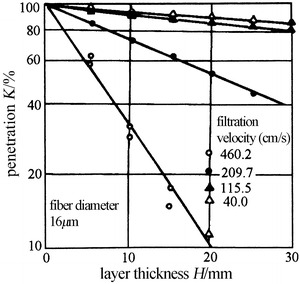
Illustration of logarithmic penetration expression

Figure 3.21 is the experimental result of the performance of thick fibrous layer with thickness 0.3–15 cm for monodisperse DOP particles, which was done by Norio and Iinoya [7]. It is shown that when the number of nominal layer H/l is less than 500, the logarithmic penetration expression is applicable.

Fig. 3.21.

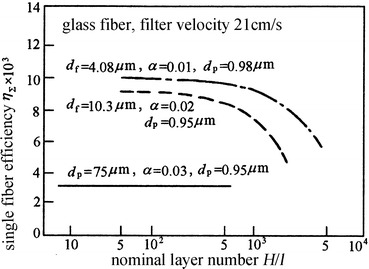
Applicability range of logarithmic penetration theory for fibrous layer

The nominal layer number is the ratio between fibrous layer thickness H and fiber spacing l. Suppose fibers are arranged in such a way shown in Fig. 3.22. Solid fraction α is the percentage of the area occupied by fibers in the area of l × l, i.e.,

Fig. 3.22.

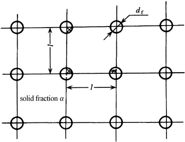
Relationship between solid fraction, fiber size, and fiber spacing

So we get:

3.47

3.48

From Fig. 3.21, the nominal layer becomes thinner for the validity of logarithmic penetration expression with the decrease of fiber diameter.

When different filtration mechanisms are concerned, a linear relationship between K and H exists in the field of diffusion when the penetration K ≥ 60 % and H is less than 20 mm while a linear relationship between K and H also exists in the field of interception and inertia when H is less than 40 mm and K ≥ 20–30 % [3].

For paper filter, the fiber structure could be thought as a fibrous layer filter after compression along the width direction. Several layers of thin papers can be overlapped for test. Different layers of overlapping represent different thickness. Several layers of thin papers can be overlapped for test. During the test, other conditions remain the same. Different layers of overlapping represent different thickness. Figure 3.23 is the result obtained by Iinoya [6]. It is shown that the single fiber efficiency ηΣ keeps the same, no matter how thick the filter paper is. The single fiber efficiency is independent of the thickness H. This means the logarithmic penetration expression is valid and the flow conditions around fibers inside filter paper are unchanged.

Fig. 3.23.

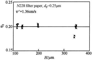
Relationship between single fiber efficiency η _Σ and filter paper thickness H

Influence of Solid Fraction

For fibrous filter with small solid fraction α, many experiments have proved that the relationship between α and efficiency fits the logarithmic penetration expression.

For filter paper, the influence of solid fraction α on logarithmic penetration expression is shown in Fig. 3.24 [6]. It is obvious that linear relationship exists between α and η _Σ for α < 0.25. When α > 0.25, single fiber efficiency η _Σ varies much. So unlike the logarithmic penetration expression, η _Σ varies with α, and the linear relationship between α and lg K does not exist. This means the effect of fiber interference becomes large. Since the solid fractions of most filter papers are less than 0.2, the logarithmic penetration expression is still valid.

Fig. 3.24.

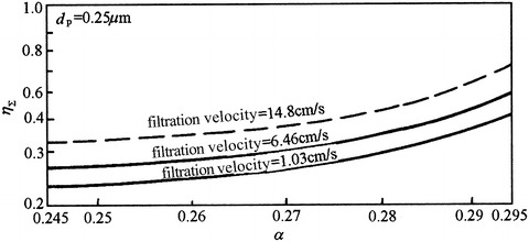
Relationship between single fiber efficiency η _Σ and solid fraction α

Influencing Factors for Efficiency of Fibrous Filters

Many factors influence the efficiency of fibrous filters, which mainly include particle diameter, fiber size, filtration velocity, and solid fraction. Now their influences are analyzed as follows.

Influence of Particle Size

When particles are polydisperse, under the role of several filtration mechanisms, smaller particles will settle onto fiber surface with diffusion. With the increase of particle size, the effect of diffusion decreases gradually. Larger particles settle onto fiber surface with interception and inertia. With the increase of particle size, both the effects of interception and inertia increase. So there is the lowest point on the efficiency curve related to particle size, which corresponds to the minimum efficiency. Particles with this size are the most difficult to be captured inside filters.

When the derivative is made on the efficiency equation of single fiber, the most penetration K _max and the particle size d _max corresponding to the minimum efficiency can be obtained.

It should be noted that d _max is not a constant value. In the past it is thought that d _max = 0.3 μm, so efficiency of HEPA filter is tested using particles with diameter 0.3 μm. But this should be linked with certain conditions. With the development of measurement techniques, many experiments have proved that d _max varies with different particles, fibers, and filtration velocities. In most cases, d _max for fibrous filters is between 0.1 and 0.4 μm. Figure 3.25 is a typical relationship between particle size and filtration for fibrous filter [17].

Fig. 3.25.

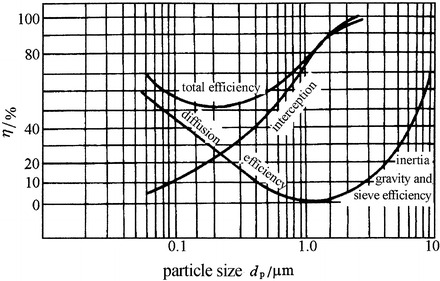
Relationship between efficiency and particle size

Next one example will be provided about the theoretical calculation of d _max [18]. When , we could get the following result based on Eq. (3.30):

3.49

where

• λ is the mean free path of air molecular (at normal temperature and pressure it is 0.065 μm);

• k is the Boltzmann constant.

The calculated results are presented in Fig. 3.26. Usually fiber diameter of HEPA filter is about 0.4 μm, solid fraction α is about 0.10, and filtration velocity is about 2.5 cm/s. From Fig. 3.26 it is clear that d _max is about 0.14 μm. d _max decreases with the increase of filtration velocity and with the decrease of fiber diameter.

Fig. 3.26.

Theoretical calculation of d _max

For α = 0.03–0.07 and d _f = 0.43–1.68 μm, the following empirical equation could be also used to estimate d _max [19], i.e.,

3.50

where the units for d _max and v are μm and cm/s, respectively.

When α = 0.07, d _f = 1 μm, and v = 2.5 cm/s, we could get d _max = 0.21 μm. If we look up Fig. 3.26, d _max is found between two straight lines and is about 0.2–0.25 μm, which means the estimate equation is useful.

Next take a look at an experiment.

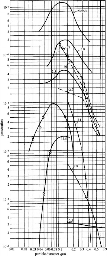
Figure 3.27 illustrates the experimental result of the influence of the filtration velocity on the most penetration for fibrous filters with d _f = 1.5 μm [4]. It is obvious that the maximum of penetration moves towards small particle size with the increase of filtration velocity.

Fig. 3.27.

Relationship between penetration and particle size under different filtration velocities

For glass fibrous filter, d _max is between 0.1 and 0.15 μm with a quite large range of filtration velocity for particles such as NaCl, DOP, and stearic acid. For PSL particles, d _max is also not 0.3 μm. Data from related literatures are presented in Fig. 3.28, which clearly illustrates this point. For experimental results are different with atmospheric dust, silver aerosol, and gold aerosol. The efficiency with 0.001–0.1 μm particles is higher than that with 0.3 μm particles, which is believed to be caused by the increased diffusional efficiency with these kinds of small particles [20].

Fig. 3.28.

Relationship between filter efficiency and particle size

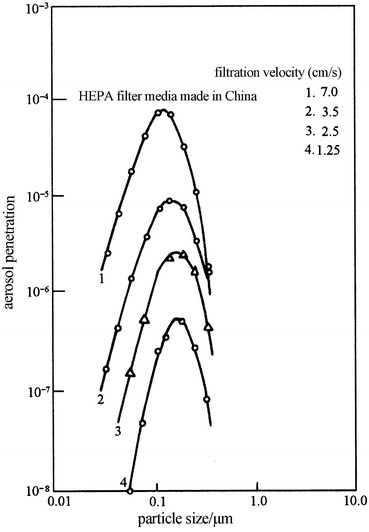
However, the most penetrating particle sizes of different fibers are different, which could be verified by the experimental results performed in the USA by the same person and same method [22]. Figure 3.29 is the penetration using DOP for common fibrous filter paper which was made in China. Figure 3.30 is the penetration using DOP for common fibrous filter paper which was made in the USA. Figure 3.31 is the penetration using DOP for ULPA filter paper which was made in China. Figure 3.32 is the penetration using DOP for ULPA filter paper which was made in the USA. It is seen that d _max is consistent with that of calculation. Tables 3.1 and 3.2 are experimental results of penetration using DOP for perchlorethylene fiber and polypropylene fiber made in China, respectively. The former d _max is about 0.08 μm, while that of the latter is 0.05 μm. According to domestic experiments, d _max for polypropylene fiber is 0.085 μm using NaCl aerosol when fiber diameter is 4 μm [23], and some test results even showed that it is 0.55 μm using atmospheric dust when fiber diameter is 6 μm [24]. This may be caused by the electrostatic effect, which will be explained later.

Fig. 3.29.

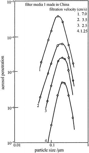
Relationship between particle size and penetration for filter media 1 (common HEPA filter) made in China

Fig. 3.30.

Relationship between particle size and penetration for filter media (common HEPA filter) made in the USA

Fig. 3.31.

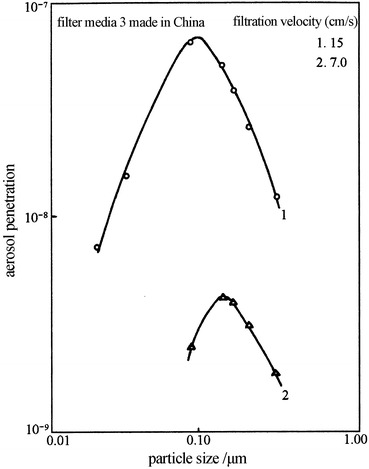
Relationship between particle size and penetration for filter media 3 (ULPA filter) made in China

Fig. 3.32.

Relationship between particle size and penetration for filter media (ULPA filter) made in the USA

Table 3.1.

Efficiency with DOP for domestic-made perchlorethylene fibrous media

△P/Pa	22.9	45.7	63.5	121.9	508.0
v/(cm/s)	1.25	2.5	3.5	7.0	13.4
Particle size/μm	Efficiency/%
0.5	–	–	–	–	97.60
0.4	99.96	99.78	99.48	98.12	96.27
0.3	99.95	99.71	99.39	97.60	95.72
0.2	99.88	99.52	99.07	97.00	92.29
0.15	99.76	99.11	98.50	96.17	91.70
0.10	99.44	98.01	96.90	93.35	87.72
0.08	99.25	97.56	96.35	93.29	88.08
0.05	99.38	97.87	96.70	93.46	87.81

Table 3.2.

Efficiency with DOP for domestic-made polypropylene fibrous media

△P/Pa	20.3	40.6	59.9	116.8	482.6
v/(cm/s)	1.25	2.5	3.5	7.0	13.4
Particle size/μm	Efficiency/%
0.5		–	–	–	99.83
0.4	99.9994	99.995	99.984	99.83	99.59
0.3	99.9991	99.990	99.970	99.71	99.12
0.2	99.9950	99.970	99.920	99.41	98.37
0.15	99.9600	99.870	99.780	98.48	97.78
0.10	99.8800	99.660	99.370	98.62	96.26
0.08	99.8500	99.560	99.270	96.52	95.39
0.05	99.8400	99.400	99.170	95.54	93.80
0.03	99.9700	99.850	99.710	98.52	–

With the increase of the efficiency of filter paper, d _max decreases. It is shown in above figures that d _max of ULPA filter paper is smaller than that of common HLPA filter. It is about 0.12 μm.

d _max is an important parameter, which is termed as the most penetrating particle size. When d _max is known and the efficiency corresponding to this particle size is assured, filtration efficiencies of particles with other sizes are guaranteed.

Because of the existing d _max, monodisperse particles with this size are needed to the evaluation of filters or polydisperse particles such as NaCl aerosols when the average diameter is close to d _max.

With the existence of d _max, filtration process of filters has the characteristic of selectivity. When particle-laden flow with polydisperse particles goes through same filters in series, particles penetrate the first filter that has the size of the most penetrating particle size or d _max. So the penetration of the second filter is larger than that of the first one. It should be noted that the ability of selectivity for single fiber with uniformly distributed mass is larger than that of fibers with nonuniform mass inside the fiber layer. For filters with damage on the surface, this ability may disappear completely.

Influence of Particle Type

Even when the particle sizes are the same, different phases have impact on the filtration efficiency. Experiment shows that efficiency for solid particle is higher than that of liquid particle, and constant efficiency is obtained for various filter media using liquid DOP particle [25]. With the increase of filtration velocity, the influence of this phase on efficiency decreases gradually.

In theory it is not clear why efficiency using solid particle is comparatively higher. Usually the following reasons are thought to cause the difference:

1. Coagulation of solid particle is more frequent than liquid one.

2. Influence of charge on solid particle is higher than that on liquid one.

3. Solid particle could significantly increase the load of filter.

4. Fibers become damaged after liquid particles are capture on the surface.

5. Error of experimental result is caused by the difference of particle size and density.

So there is some people advocate to test filters using solid particles, which is thought to give real result. However, others prefer to use liquid particle for the test for safety.

Influence of Particle Shape

Particles used for efficiency test of air filters as well as for efficiency calculation are spherical. Contact surface area for spherical particles touching fibers is smaller than that of irregularly shaped particles. So the probability of contact with fibers for irregularly shaped particles is larger, which makes the probability of deposition larger. In fact atmospheric particles are irregular shaped, so the real filtration efficiency is larger than that of calculation and experiment. The largest penetration for spherical particles is safe.

Influence of Fiber Size and Cross-Sectional Shape

According to the aforementioned filtration mechanisms, filtration efficiency increases with the decrease of fiber size. For comparison purpose, results from Figs. 3.29, 3.30, 3.31, and 3.32 are listed in Tables 3.3, 3.4, 3.5, and 3.6 [22]. It is shown that since diameters of fibers in the domestic-made fibrous filter paper are smaller than that made in the USA, the former efficiency is much higher. Therefore, smaller fibers are preferred during the selection of HEPA filter media. Of course the pressure drop of filter will increase with the decrease of fiber size.

Table 3.3.

Penetration of HEPA filter media 1 made in China and common HEPA filter media made in the USA

Filtration velocity/(cm/s)	Chinese filter media l		UK filter media
	Particle size/μm		Particle size/μm
	0.1	0.3	0.1	0.3
1.25	3.25 × 10−7	2.02 × 10−6	3.30 × 10−6	3.20 × 10−6
2.50	3.64 × 10−6	1.00 × 10−5	5.40 × 10−5	2.50 × 10−5
3.50	1.53 × 10−5	2.26 × 10−5	1.20 × 10−4	3.80 × 10−5
7.00	1.41 × 10−4	5.30 × 10−3	8.50 × 10−4	1.50 × 10−4

Table 3.4.

Fiber diameter of HEPA filter media 1 made in China and common HEPA filter media made in the USA

Fiber	Chinese filter media l	UK filter media
The coarsest fiber/μm	4.00	5.60
The finest fiber/μm	0.12	0.20

Table 3.5.

Penetration of ULPA filter made in China and the USA

Filtration velocity/(cm/s)	Chinese filter media		UK filter media
	Particle size/μm		Particle size/μm
	0.13	0.29	0.13	0.29
7.0	3.27 × 10−9	1.91 × 10−9	2.53 × 10−5	1.32 × 10−5
1.50	5.1 × 10−8	1.25 × 10−8	–	–

Table 3.6.

Fiber diameter of ULPA filter media made in China and the USA

Fiber	Chinese filter media	UK filter media
The coarsest fiber/μm	0.73	2.5
The finest fiber/μm	0.04	0.10

Influence of fiber cross-sectional shape on filtration efficiency is not large, which is shown in Fig. 3.6. Although correction factors for shape were proposed by Haya, it is usually ignored because of computational complexity [26].

Influence of Filtration Velocity

Like the most penetrating particle size, there is the most penetration filtration velocity for each filter. Qualitative relationship among several filtration mechanisms, filtration velocity, and other parameters is illustrated in Fig. 3.33. The figure illustrates that:

1. Diffusion efficiency decreases with the increase of filtration velocity.

2. Inertial efficiency increases with the increase of filtration velocity.

3. Interception efficiency increases with the increase of filtration velocity.

4. With the increase of filtration velocity, the total efficiency decreases at first and then increases. So there is a filtration velocity for the minimum efficiency or the maximum penetration.

Fig. 3.33.

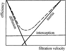
Influence of filtration velocity on various efficiencies

Figure 3.34 illustrates the quantitative relationship between efficiency of single fiber and filtration efficiency [27]. For example, for fiber with diameter 20 μm and particles with diameter 7 μm, the filtration velocity corresponding to the maximum penetration is about 0.8 m/s, while it is 0.2–0.3 m/s for particles with diameter 2 μm. It is advisable to choose suitable filtration velocity during the design of air filters, given the size range of particles captured and fiber diameters.

Fig. 3.34.

Influence of filtration velocity on singe fiber efficiency

Figure 3.35 presents the relation curve between filtration efficiency and filtration velocity for two filter papers using methylene blue particles (the mass median diameter is 0.6 μm), which was performed at Institute of HVAC of China Academy of Building Research. It is shown that efficiencies of two filter papers at low filtration velocity (below 0.2 m/s) are quite high, and both efficiencies decrease with the increase of filtration velocity. At filtration velocities 0.7 and 0.9 m/s, filtration efficiencies for synthetic fiber paper and glass fiber paper arrive at the minimum, respectively. When filtration velocities are larger than these respective critical values, both efficiencies of filter papers increase. It is shown from Figs. 3.29, 3.30, 3.31, and 3.32 that efficiency for HELA or ULPA filters will increase by an order of magnitude when filtration velocity decrease from 2.5 cm/s to half. It is not cost-effective to increase the filtration area by two times or reduce half of the flow rate. At present, the practical filtration velocity is mainly 2.5–3 cm/s.

Fig. 3.35.

Relationship between efficiency and filtration velocity of two filter papers

Moreover, it is shown from Fig. 3.34 that for particles with diameter 0.3 μm, the penetration of fiber layer with fiber diameter 20 μm reaches maximum when filtration velocity is larger than 1 m/s. In Fig. 3.27 we could see that for filtering particles with the same diameter, the filtration velocity corresponding to the maximum penetration reduced to 0.2 m/s for fiber layer with fiber diameter 1.5 μm.

So we could see the trend that filtration velocity corresponding to the maximum penetration for the fiber with same diameter increases with the decrease of particle size. For particles with the same diameter, the filtration velocity corresponding to the maximum penetration increases with the increase of fiber diameter.

For filtration velocity below 0.1 m/s, it is common that penetration decreases with the decrease of filtration velocity. However, this law is much obvious for particles with diameter <0.5 μm than that of >0.5 μm. This characteristic is more prominent for smaller particle size [20]. This may be caused by the intense diffusion effect of smaller particles at small filtration velocity.

For polypropylene fibers, the relationship between penetration and filtration velocity is clear: penetration will increase four times when filtration velocity increases 2 times, which is shown in Fig. 3.36. The relationship could be expressed as . Filters made of this kind of material have the similar conclusion, which is shown in Fig. 3.37 [28]. This law is also proved by others’ experiment [23]: penetration increases by 50–100 times when filtration velocity increases by 10 times. Within the common low filtration velocity range, the change is comparatively large. While in the range of high filtration velocity, the change is small and gradually goes towards a limit value, which is shown in Fig. 3.38.

Fig. 3.36.

Relationship between penetration and filtration velocity for polypropylene media

Fig. 3.37.

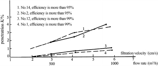
Relationship between penetration and filtration velocity for sub-HEPA filter

Fig. 3.38.

Relationship between penetration and specific velocity (sodium flame method)

Influence of Solid Fraction

Experiments [4] have shown that the relationship between solid fraction and efficiency is:

3.51

3.52

3.53

Influence of solid fraction on total efficiency of single fiber inside filters is as shown in Eq. (3.35), i.e.,

It is shown that fiber layer becomes dense when solid fraction increases, which increases inertial efficiency and interception efficiency. On the contrary, since the filtration velocity inside the space between fibers increases, diffusion efficiency decreases. However, the total efficiency still increases. It should be noted that the increase speed of pressure drop is quicker than that of the total efficiency, so it is not reasonable to increase the total efficiency by increasing the solid fraction α.

Influence of Air Temperature

Diffusion coefficient of particles will increase with the increase of air temperature, which elevates the diffusion efficiency of submicron particles. However, air viscosity will be enlarged by the increase of air temperature, which reduces the deposition efficiency of large particles by gravitational and inertial effects and at the same time increases the pressure drop of filters.

Influence of Air Humidity

Penetration will increase with the increase of air humidity, which decreases the efficiency. For the filter paper made of glass fiber bound with phenol-furfural resin, experiment was performed on it to obtain the performance of bacterial capture efficiency. It is shown that the bacteria can penetrate deeper into the wet filter paper than into the dry filter paper [29]. When saturated water vapor goes through filters made of glass fiber paper, iron rust carried by vapor can penetrate deeper through several layers of filter papers. While dry air is used, the iron rust is only found on the surface of filter. The reason for efficiency decrease by lower humidity is that electrostatic effect disappears by wet air and Brownian motion is weakened, which makes the air carry away particles to further penetrate.

Influence of Airflow Pressure

The decrease of air pressure will reduce air density and enlarge mean free path of air molecules, which increase the slip correction coefficient. Both diffusion coefficient and inertial parameter will increase, so both diffusion and inertial efficiencies increase. It has little effect on the interception efficiency.

When both air temperature and pressure increase at the same time, inertial efficiency will decrease, because the influence of the increase of pressure on viscosity is larger than that of temperature.

Influence of Dust Holding Capacity

As the deposition process of particles on fiber surface goes on, the dust loaded on filers increases gradually, and the second stage of filtration starts. The shape of deposited particles on fibers is similar as that of deposited snow and ice crystal. They are called dendrite crystal model [30, 31]. Filtration efficiency increases with the increase of particles deposited.

In 1946 the shape of dendrite crystal on single fiber with monodisperse latex particles has been discovered. Thirty years later, the first computer model was set up for modeling two-dimensional dendrite crystal structure on circular cylinder in a microscopic scale, which is a breakthrough progress [32]. Both figures cited from Ref. [2] and Fig. 3.39 present this kind of dendrite crystal structure vividly for used filters. Generally forming of the dendrite crystal shape is much obvious for comparatively small fiber and comparatively large particle, which are shown in Figs. 3.39 and 3.40c–f (see Ref. [2]). It is difficult to find this kind of structure for large fiber and small particle. They are like the appearance of rough tree rind, which is shown in Fig. 3.40a, b.

Fig. 3.39.

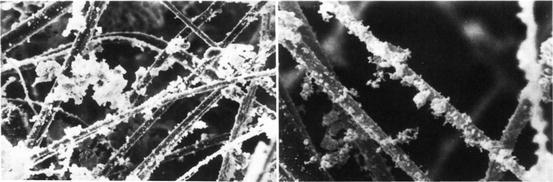
Particle coagulation on filter medium

Fig. 3.40.

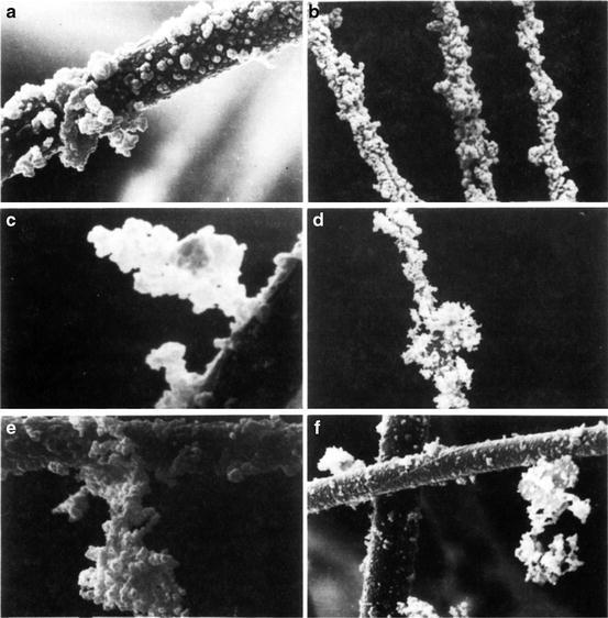
Coagulation of deposited particles on fibers

If the microscopic photo of coal dust on Fig. 2.9 is understood, the forming of this kind of dendrite crystal structure will not be unimaginable.

Because of the blockage of deposited particles, both efficiency and pressure drop will increase.

But the above dendrite crystal model overestimates the increase of efficiency of used filters, so the lifetime of filters is underestimated. The reasons are as follows:

1. In this model the dendrite structure can only be formed upstream. Fibers are thought rigid, while they can bend in reality. In fact, particles captured will extend in radial direction. So when dendrite is formed along one direction, the flow path will be blocked immediately, which increases both efficiency and pressure drop suddenly and ends the lifetime of filters.

2. Flow field around fibers is assumed constant in this model. This will increase the efficiency unrealistically. Actually flow field near the captured particles will vary or increase with the increase of dust loading.

3. Resuspension of deposited particles from fiber surface is not considered.

Given the above shortcomings, dendrite fiber model was put forward, which could save the computational time [33]. In this new model, particles captured will be thought as the extra fiber added to the filter media. The problem of radial formation of dendrite structure is solved. Computers with high efficiency are used to solve the flow field. So dendrite fiber model is closer to reality than dendrite crystal model, which estimates long lifetime of filters. But the shortcoming of dendrite fiber model is that it cannot provide the figure of single dendrite structure. As for the problem of resuspension, further theoretical study is still needed.

The calculation method of efficiency and pressure drop after dust loading can be referred to Ref [2]. Although efficiency after dust loading increases, most studies of this phenomenon only have theoretical implication. In face efficiency for new filter is used for safety.

Capillary Model Theory

Fibrous filters have low solid fraction, while membrane filters have high solid fraction. There are two types of membrane filters including porous type and capillary type. Porous membrane and microporous membrane are introduced in 10.1007/978-3-642-39374-7_4. They have pore structure similar as foam plastic, where holes are linked together like network. Their performance is the same as fibrous filter when their thickness and density are the same and effective fiber diameter is slightly less than pore diameter. For example, membrane filter with pore diameter 0.8 μm is equivalent with fibrous filter with effective fiber diameter 0.55 μm. According to calculation, the pressure drop is the same as that of fibrous filter [34].

Another kind of membrane filer is Nuclepore membrane filter which will be described in detail in 10.1007/978-3-642-39374-7_4. Capillary model is more suitable to describe its performance. Pores inside Nuclepore membrane filter are independent from each other, while fibers inside fibrous filters have interference connections. In capillary model, circular parallel pores with diameter d _f are placed equidistantly. They are perpendicular to the membrane surface. The length equals with the membrane thickness. In real situation there is still a small angle between pore axis and normal direction of membrane surface, which is smaller than 15°.

Figures 3.41 and 3.42 are chemical microporous filter membrane and Nuclepore membrane filter, respectively [35].

Fig. 3.41.

Surface of microporous membrane

Fig. 3.42.

Surface of Nuclepore membrane filter

Hagen-Poiseuille law is used to describe the continuum flow inside capillary [36], i.e.,

3.54

Correction should be considered in the range of small Knudsen number (see Table 6.3), i.e.,

3.55

where r _f is the pore radius, n is the pore number, and K _n is the Knudsen number, , where λ is the mean free path of air molecule.

Equation (3.55) has the similar form as Eq. (4.15). Pressure drop is proportional to the flow velocity or flow rate. Domestic experiment has shown that linear proportional relationship exists in the range of face velocity ≤9 cm/s, which is shown in Fig. 3.43 [37]. Pore radiuses in this figure are: (1)  μm, (2) μm, (3) μm, (4) μm, and (5) μm.

Fig. 3.43.

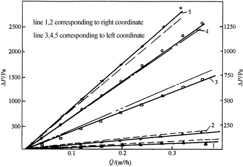
Variation of pressure drop of Nuclepore membrane filter with filtration flow rate

Efficiency expression based on capillary model is [38]:

3.56

where

3.57

3.58

3.59

3.60

Expression of St is the same as Eq. (3.7), except that D _f is the pore size, not particle size; and d _p is the particle size, not fiber size.

When dimensionless parameter ,

3.61

where H is the pore length and D is the diffusion coefficient of particles.

When N _d > 0.03

3.62

3.63

where N _r is the interception parameter of capillary

3.64

where D _f and d _p are defined the same as Eq. (3.60). Interception parameter R here is slightly different from the previous mentioned one. In Eq. (3.56), the parameter 0.15 was obtained by measurement with Nuclepore membrane filter. This equation usually underestimates the interception efficiency because only the flow on the pore face is considered.

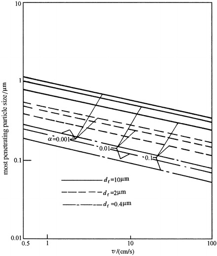
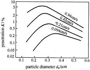
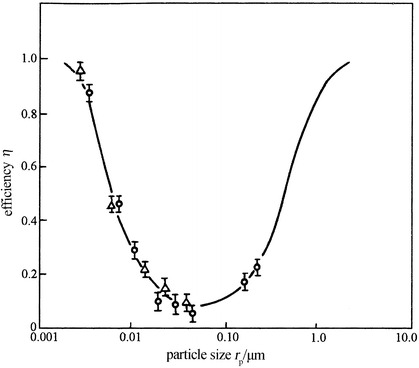
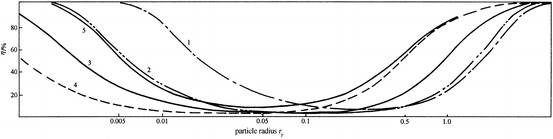
Figure 3.44 presents the curve of theoretical calculation using the above equation, which fit quite well with experimental data [39]. Figure 3.45 was obtained through theoretical calculation by domestic researcher [40], from which we can see that the curve moves left with the increase of filtration velocity. The reason may be the combined effect of increased collision efficiency with decreased diffusion efficiency. Consistency between the two theoretical calculation results could be found when two curves are plotted together, which is shown in five of the latter figure.

Fig. 3.44.

Comparison between efficiencies of theoretical calculation and experimental data on Nuclepore membrane filter (condition: D _f = 5 μm, v = 5 cm/s)

Fig. 3.45.

Comparison between the theoretical calculation result from domestic researcher and the result abroad for the efficiency of Nuclepore membrane filter (condition: D _f = 8 μm, ρ _p = 2,000 kg/m³, porosity is 5 %) 1. v = 0.1 cm/s, 2. v = 1.0 cm/s, 3. v = 8.0 cm/s, 4. v = 16.0 cm/s, 5. plot with theoretical curve by Fig. 3.44

Efficiency of Granule Air Filter

When granule air filter is used to capture particles in the airflow, the filtration mechanisms are similar as that of fibrous filter. For the convenience of reference, the total efficiency expression is given [41]:

3.65

where

• η is the total efficiency of granular filling layer;

• L is the thickness of granular filling layer;

• d _c is the granular diameter;

• α is the granular solid fraction:

η′ is the efficiency of single granule. The respective effect is introduced below:

Diffusion efficiency is:

3.66

3.67

Direct interception efficiency is:

3.68

Inertial efficiency is determined with inertial parameter St. Numerical solution to inertial efficiency with St based on layer porosity (1–α) as a parameter is presented in Fig. 3.46. However, the difference between theoretical value and experimental data is still large.

Fig. 3.46.

Comparison between theory and experiment for inertial efficiency of granular filter

References

- 1.Takizawa S Air filter in the pharmaceutical industry. J Jpn Air Clean Assoc. 1994;32(2):28–38. [Google Scholar]
- 2.Cai J . Fibrous filters with non-ideal conditions. Stockholm: The Royal Institute of Technology; 1992. p. 119. [Google Scholar]
- 3.Niitsu Y, Yoshikawa S, Kubo T Study on the filtration of ultrafine particles. J SHASE Jpn. 1972;46(9):13–19. [Google Scholar]
- 4.Ужов ВИ, Мягков БИ, Очистка промышленных гаэов фильтрами, Москва (1970) (In Russian)
- 5.Сгечкина ИБ, Кирш АА, Фукс НА, Исследования В области волокнистых Азрозольных Азрозольных фильтров, Коллоидный журнал (1969), pp 121–126 (In Russian)
- 6.Kouichi I, Makino K, Inoue O, et al. Particle capture performance of filter paper. J Chem Eng Jpn. 1970;34(6):632–637. [Google Scholar]
- 7.Kimura N, Koichi I Particle capture efficiency of single fiber in the filling layer of glass fibrous filter. J Chem Eng Jpn. 1965;29(7):538–546. [Google Scholar]
- 8.Yoshikawa S Air filtration – analysis case of filter structure and its application. J SHASE Jpn. 1978;52(5):47–55. [Google Scholar]
- 9.Richard D (1981) Aerosol handbook (trans: Zhou Jinqin), pp 82–83 (In Chinese)
- 10.Davies CN. The separation of airborne dust and particles. Proc Inst Mech Eng. 1952;1B:185. [Google Scholar]
- 11.Yoshioka N, et al. Filtration of fibrous filling layer – collisional efficiency in low Re flow. J Chem Eng Jpn. 1967;31(32):157–163. [Google Scholar]
- 12.Кирш АА, Стечкина ИБ, Фукс НА, Исследования В области волокнистых Азрозольных Азрозольных фильтров, Коллоидный журнал (1969) pp 227–232 (In Russian)
- 13.Chen CY. Filtration of aerosol by fibrous media. Chem Rev. 1955;55(4):595–623. doi: 10.1021/cr50003a004. [DOI] [Google Scholar]
- 14.Kamishima K Air cleanliness level in cleanroom with 0.1μm particles as the study object. Jpn Air Condit Heat Refri News. 1981;21(5):91–99. [Google Scholar]
- 15.Zhou B, Zhang XS Investigation of logarithmic penetration expressions for fibrous media. Build Energy Environ. 2011;30(1):63–65. [Google Scholar]
- 16.Yoshikawa S Air filtration (1) – filter structure. J SHASE Jpn. 1978;52(4):69. [Google Scholar]
- 17.Engle PM, Bauder CJ. Characteristics and application of high performance dry filters. ASHRAE J. 1964;6(5):72–75. [Google Scholar]
- 18.Tolliver DL (1993) Handbook of contamination control in microelectronics: principles, applications and technology (trans: Yu Aoyuan et al.), pp 29–30 (In Chinese)
- 19.Cheng XY, Zhang JK, Shi XC, et al. Penetration and the most penetrating particle size. Contamin Control Air-Condit Technol. 1990;1:17–26. [Google Scholar]
- 20.Filtration Special Committee of Japan Nuclear Fuel Service Experimental study of the safety of HEPA filter used in nuclear fuel facilities. J Jpn Air Clean Assoc. 1980;18(3/4):2–23. [Google Scholar]
- 21.Ventilation Committee and Subcommittee on Dust Measurement Method Measurement method of airborne particles in Buildings (2) GA JAPAN. 1975;90(1098):849–866. [Google Scholar]
- 22.Liu BYH, Lin B. Performance test of domestic air sampler and high efficiency filter media. Contamin Control Air-Condit Technol. 1987;3:9–14. [Google Scholar]
- 23.Zhang JK, Ouyang T, Cheng XY (1986) Performance of polypropylene fibrous filter media. In: Proceedings of the second annual academic conference by Chinese Contamination Control Society, pp 157–161 (In Chinese)
- 24.Fan CY, Lin ZP. Properties of sub-high efficiency polypropylene filter media. Proceedings of the biennial meeting of China HVAC&R, Zhangjiajie, October. 1994;1994:159–162. [Google Scholar]
- 25.Stafford RG, Ettinger HJ. Comparison of filter media against liquid and solid aerosols. Am Ind Hyg Assoc J. 1971;32(5):319–326. doi: 10.1080/0002889718506467. [DOI] [PubMed] [Google Scholar]
- 26.Kimura N, Kouichi I Particle capture performance of fibrous filling layer filter and influence of fiber cross sectional shape. J Chem Eng Jpn. 1969;33(10):1008–1013. [Google Scholar]
- 27.Emi H Particle capture efficiency of air filter. Chem Ind. 1975;19(3):209–215. [Google Scholar]
- 28.Xu ZL, Shen JM (1987) YGG and YGF type low resistance sub-high efficiency air filter. Research report of Building Science, China Academy of Building Science Research, 5–2 (In Chinese)
- 29.Huang ZL, Hui CR. No. 1 soft leather treatment agent for treating with ultra-fine glass fibrous paper for air filtration. Chin J Antibiot. 1979;4(4):15–17. [Google Scholar]
- 30.Payatakes AC. Model of aerosol particles deposition in fibrous media with dendrite-like pattern-application to pure interception during period of unhindered growth. Filtrat Separat. 1976;13(6):602–608. [Google Scholar]
- 31.Kanaoka C, Emi H, Myojo T Simulation of aerosol loading process on fiber surface. Proc Soc Chem Eng Jpn. 1978;4(5):535–537. [Google Scholar]
- 32.Cai J (1992) Fibrous filters with non-ideal conditions. The Royal Institute of Technology, Stockholm, 2992, p 137
- 33.Cai J (1992) Fibrous filters with non-ideal conditions. The Royal Institute of Technology, Stockholm, 2992, pp 195–218
- 34.Hinds WC (1989) Aerosol technology (trans: Sun Yufeng, Chapter 9). Heilongjiang Science and Technology Press, Harbin (In Chinese)
- 35.Shi XC (1986) Study of nuclepore membrane filter structure and its filtration performance. Tsinghua University, p 11 (In Chinese)
- 36.Tolliver DL (1993) Handbook of contamination control in microelectronics: principles, applications and technology (trans: Yu Aoyuan et al.), pp 37–38 (In Chinese)
- 37.Shi XC (1986) Study of nuclepore membrane filter structure and its filtration performance (Master dissertation). Tsinghua University, p 13 (In Chinese)
- 38.Tolliver DL (1993) Handbook of contamination control in microelectronics: principles, applications and technology (trans: Yu Aoyuan et al.), China Aerospace Architectural Design Academy, pp 39–40 (In Chinese)
- 39.Tolliver DL (1993) Handbook of contamination control in microelectronics: principles, applications and technology (trans: Yu Aoyuan et al.), p 41 (In Chinese)
- 40.Shi XC (1986) Study of nuclepore membrane filter structure and its filtration performance (Master dissertation). Tsinghua University, p 52 (In Chinese)
- 41.Richard D (1981) Aerosol handbook (trans: Zhou Jinqin). Atomic Energy Press, Beijing, pp 83–84 (In Chinese)