Airborne Particles in Outdoor Air: Atmospheric Dust

Abstract

Atmospheric dust is the direct treatment object in air purification system. We should understand not only the concept of atmospheric dust in air clean technologies but also its origin, component, concentration, and distribution.

Atmospheric dust is the direct treatment object in air purification system. We should understand not only the concept of atmospheric dust in air clean technologies but also its origin, component, concentration, and distribution.

Once the general characteristic of particle size distribution is understood, other characteristics of the airborne particles in outdoor air, i.e., atmospheric dust, are facilitated for further research.

Concept of Atmospheric Dust

The generalized meaning of atmosphere refers to all the air surrounding the earth. Special atmosphere refers to the outdoor air which person and matter are exposed to, namely, the environmental air.

Atmospheric particles are generally referred to atmospheric aerosol, while they are called atmospheric dust specifically.

Atmospheric dust can also be divided according to the special and the generalized meanings.

At early days, the concept of atmospheric dust refers to the airborne solid particles [1], i.e., the real dust, which is the special meaning of the atmospheric dust. Later someone such as Junge from Germany put forward the concept that the atmospheric dust is the aerosol with coarse diameter [1]. But this concept is not complete [2], because aerosol with high degree of dispersion can be generated using artificial method or natural method occurred in atmosphere. Therefore, the modern concept of atmospheric dust refers to not only the solid dust, but also the polydisperse aerosol containing both solid and liquid particles, which is the generalized concept of atmospheric dust. It means the particles with size (refers to the aerodynamic diameter) less than 10 μm. It is called the floating dust in the environmental protection field, which is different from the deposition dust that deposits onto the floor within a short time. So the concept of the atmospheric dust in the field of air cleaning technology is different from that of the dust in the field of general dust removal technology. The generalized concept of atmospheric dust in the field of air cleaning technology is suitable for the modern technology of particle measurement. Because with the method of photoelectricity, both solid and liquid particles can be detected to obtain the relative concentration or the number concentration of atmospheric dust. Corresponding to this generalized concept of atmospheric dust, particles with diameter less than 10 μm are called “airborne particulate matter” and “environmental aerosol” which were specified in EPA of the USA and special committee from environmental standard related to airborne dust in Japan, respectively. This is the general term for airborne dust and airborne particles [3].

The total suspended particles (TSP) mentioned in Chinese standard “Ambient Air Quality Standard” include both the airborne particles with diameter less than 10 μm and the deposition particles with diameter between 10 and 100 μm. In the past, airborne particles with diameter less than 10 μm were called floating dust, and now they are called inhalable particles (IP) and labeled as PM₁₀. In the field of environmental science, particles with diameter less than 2 μm or 2.5 μm are called fine particles, while others are called coarse particles. In American standard, TSP only includes those with diameter between 0 and 40 μm.

Except for the original particles (from the particle generation source), the concept of atmospheric dust also includes the secondary particles. The secondary particles are generated by condensation of gaseous pollutants discharged from various pollution sources, and complex chemical reaction occurred in atmosphere.

Gaseous pollutants in atmosphere include:

The formation of secondary particles is mainly sulfate, nitrate, and semi-volatile organic compounds. Among them, sulfate is very stable while both nitrate and semi-volatile organic compounds transform between gas and particle phase with the temperature. For example, when the temperature is below 15 °C, most nitrates exist in the form of ammonium nitrate particles. That is why the concentration of this kind of particle is much higher in winter when compared with summer.

The aerodynamic diameter of those secondary particles mentioned above are mainly below 2.5 μm, expressed as PM2.5, and it is the frontier of the research about atmospheric dust.

Source of Atmospheric Dust

Natural Source and Artificial Source

Atmospheric dust comes from natural and artificial sources.

There are many kinds of natural sources. There are sea salt particles which are brought into the air by the effects of sea spray, which can pass through the land for hundreds of kilometers and 90 % of which will be deposited into the sea. There are soil particles blown up by winds. There are plenty of particles released from forest fire and volcanic eruption. There are also meteoric shower in the universe and botanic pollen.

As for the artificial source, atmospheric pollution created by the development of modern industrial technology plays the most important role. Western countries have begun the era of air pollution as they used the coal instead of wood in the fourteenth century, which belongs to the soot type and the first stage in air pollution. Ash component occupies a large proportion of coal as the fuel, and usually it is about more than 20 % by weight, while petroleum has much fewer component of ash. Although soot has became fewer and fewer after petroleum took the place of coal, the generated sulfur dioxide has been converted into sulfuric acid mist through the complex reaction caused by sunlight, when it comes across moisture at high altitude in the air. This kind of fuel oil pollution is the second stage of air pollution. With the further development of fuel oil industry and the increasing amount of motor vehicles, the frequency of photochemical oxidant increases sharply. This is a series of complex reactions between nitrogen oxides and hydrocarbons exhausted from combustion. Ozone, peroxyacyl nitrate, and other substances will be generated. These substances produce a kind of toxic smoke through the radiation of solar ultraviolet. This begins the era of photochemical smog, which is the third stage of air pollution. Although photochemical reaction can be avoided when diesel engine is used and few hydrocarbons are generated, smog is still formed.

It is an important source of evidence that the change of the amount of dust and lead content measured from ice in the Arctic is caused by the industrial development of the modern capitalism. Heavy metal element such as lead is a good tracer material in showing atmospheric transmission path.

Figure 2.1 indicates the change of dust content in ice sample between the early nineteenth century to the 1960s [4]. After 1930, the content of dust in ice sample increased sharply which is consistent with the trend of energy abusing after this period in capitalist countries.

Fig. 2.1.

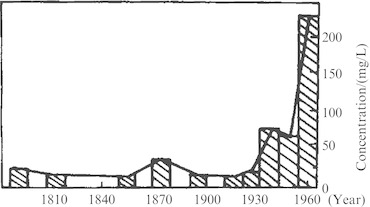
Change of dust content in ice sample

The upper curve of Fig. 2.2 [4] shows the change about the annual yield of the lead refining industry in the Northern Hemisphere. The lower curve shows the change of lead in ice of the Arctic. In 800 B.C., 1 g of ice contained 0.001 μg of lead, but it increased from 200 years ago. The ice sample is taken from the hinterland of Arctic, while most lead refining industry is in the middle latitude of Northern Hemisphere. We can see from the picture that the trend of the two curves is also very consistent.

Fig. 2.2.

Change of lead content in the ice of Northern Hemisphere

According to the newspaper, Chinese scientists’ investigation of lead content in the Arctic Center District shows that pollution has accounted for more than 90 % of the content of lead in Europe, Northern and Western America, and Central Russia and the Far East [5].

In addition to the refining production of lead mentioned above, atmospheric dust sources related to industrial pollution are mainly specified in Table 2.1.

Table 2.1.

Pollution sources of atmospheric dust

Generation apparatus	Dust property
Boiler	Coke button, fly ash, pulverized coal
Cement kiln	Mountain flour, cement
Ore sintering furnace	Metal sulfur oxide, fly ash, mineral flour
Ore furnace	Mineral flour, coke flour, slag
Steelmaking open hearth	Ferric oxide
Kiln	Fly ash, pulverized coal
Converter	Residual
Waste burning furnace	Residual, fly ash, breeze
Vitriol equipment	Sulfurous smog
Ore crushing equipment	Mineral flour

In China, the anthropogenic source of atmospheric dust mainly comes from soot pollution, which can also be seen from Table 2.2 [6]. Coal has been the most important part of energy consumption in China. According to the 2001 China Environment Yearbook (published by the China Environment Yearbook Press), the amounts of coal and oil consumed in the year 2000 are 81,188 × 10⁴ t and 2,890 × 10⁴ t, respectively. What’s more, when the scattering effect of solar radiation by the wind and water vapor is excluded, the turbidity factor reflecting the turbidity by atmospheric aerosol can be obtained, which has consistent trend with consumption of coal used in industry as shown in Fig. 2.3 [7]. There is one exception in the year 1965 shown in this figure. Because there were many rainy days that year, so most dust had been cleared.

Table 2.2.

Primary energy consumption and its constitution in 1989

	World	China	USA	USSR	Federal Republic of Germany	France	UK	Japan
Consumption/utcD	11,447.1	969.3	2,927.8	2,023.0	383.5	299.4	285.6	630.7
Oil	38.3	17.2	41.9	31.3	40.3	42.8	34.9	57.8
Natural gas	21.3	2.1	24.0	39.6	17.0	12.0	23.6	10.2
Coal	27.8	75.8	23.3	20.9	27.6	9.4	31.6	17.8
Hydroelectricity	7.0	4.9	3.5	6.3	1.4	33.8	2.2	4.7
Nuclear power	6.6		7.0	6.3	12.5	33.8	7.7	9.5
Others			0.3	1.9	1.2	2.3
In total	100.0	100.0	100.0	100.0	100.0	100.0	100.0	100.0

Fig. 2.3.

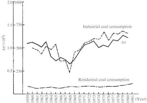
Relationship between the turbidity factor Δτ of atmospheric aerosol and coal consumption for 20 years in one industrial city

Generation Amount of Atmospheric Dust

Estimation of the generation amount of atmospheric dust from various sources is quite different. For example, estimations of the amount of dust from wind can differ by 10 times. Among the artificial sources, estimations of the amount from coal can also differ by several times. Because at present 3 kg of coal dust will be emitted into the atmosphere during the burning of 1 t coal, however, it will reach 11 kg when incomplete combustion.

Table 2.3 is an estimation for the amount of dust created by different sources. We can see from the table that 70 % of atmospheric dust in the air is produced by wind, while artificial sources only occupies for 6 %. This is because the small value for the amount of industrial pollution is used. Otherwise, given the large proportion of sea aerosol deposition into the sea, atmospheric dust generated by industrial pollution sources will reach up for 25–30 % of the total amount.

Table 2.3.

Generation amount of atmospheric dust

Type of dust source			Generation rate (t/d)	Percentage (the maximum)
Natural source	Direct	Sea salt particle	3 × 106	28
		Wind dust	2 × 104 – 106	9.3
		Forest fire	4 × 105	3.8
		Volcanic eruption	104	0.09
		Meteoric dust	5 × 10 – 5.5 × 102
	Indirect	Botanic activity (such as pollen release)	5 × 105 – 3 × 106	28
		Circulation of sulfur and nitrogen	3 × 106	24.1
	Subtotal		10.1 × 106
Artificial source	Direct	Combustion and industry	1–3 × 105	2.8
		Wind dust (by farming)	102 – 103	0.009
	Indirect	From component with aerosol generator	3.7 × 105	3.453
	Subtotal		6.7 × 105
In total			10.7 × 106

According to the report from UNEP, the amount of emissions of total suspended solids between 1982 and 1984 is 1.35 × 10⁸ t per year. Now there are also three hundred million tons of SO₂ and 1.5 × 10⁴ t nitrogen oxides emitted into the atmosphere. Among those emissions, 2.7 × 10⁸ t takes place in the USA [9].

Tables 2.4 and 2.5 show the specific emissions of SO₂, soot, and dust in different industries from different provinces in China in the year 2000 [10].

Table 2.4.

Situation of exhausted gas emission from different provinces (in 2000), unit: t

Area	Industrial SO2 emission			Removal of industrial smoke dust	Release of industrial smoke dust	Removal of industrial dust	Release of industrial dust
	Total	From combustion exhaust	From industrial process exhaust
Beijing	146,431	143,708	2,723	1,357,227	51,842	996,605	93,681
Tianjin	213,709	208,857	4,852	2,312,175	112,234	234,231	37,911
Hebei	1,133,599	960,479	173,120	7,195,272	672,176	2,979,927	812,663
Shanxi	902,681	748,396	154,285	6,416,287	791,100	1,771,044	504,133
Inner Mongolia	506,309	452,201	54,107	4,528,710	303,292	587,030	175,644
Liaoning	705,672	592,624	113,047	8,610,888	547,223	3,087,312	429,231
Jilin	201,688	176,371	25,317	4,544,264	283,006	1,161,732	123,792
Heilongjiang	221,670	208,186	13,484	6,428,612	409,337	502,422	103,853
Shanghai	326,804	319,895	6,910	3,083,548	83,153	2,180,813	26,941
Jiangsu	1,140,991	1,050,967	90,024	7,254,087	374,737	2,104,759	256,790
Zhejiang	561,847	510,230	51,616	4,195,609	247,096	2,049,220	489,627
Anhui	350,625	277,820	72,805	3,362,890	243,493	1,352,453	284,977
Fujian	214,338	191,303	22,134	1,320,414	103,539	1,346,911	187,076
Jiangxi	288,108	216,013	27,099	2,893,533	234,059	1,223,416	343,351
Shandong	1,460,902	1,383,218	77,684	9,027,355	543,067	5,059,711	745,589
Henan	747,384	635,699	111,685	7,182,665	690,618	2,927,880	817,734
Hubei	508,218	406,499	101,719	2,215,959	321,461	2,331,507	410,286
Hunan	626,494	402,091	224,403	2,007,277	381,268	1,737,738	639,667
Guangdong	881,556	805,697	75,859	5,704,256	264,453	2,517,735	579,895
Guangxi	800,485	646,803	153,682	2,435,335	590,999	2,668,408	567,717
Henan	20,178	17,459	2,719	231,497	18,078	121,642	13,470
Chongqing	664,240	640,615	23,625	1,457,313	121,783	446,098	220,127
Sichuan	994,064	865,646	128,417	2,284,428	798,910	1,852,488	559,794
Guizhou	642,490	576,358	66,132	2,780,444	342,453	480,781	406,234
Yunnan	323,853	258,732	65,123	1,496,724	232,566	1,073,720	122,818
Xizang	756	453	303	613	1,150	14	2,114
Shanxi	553,738	508,220	45,519	2,477,843	371,908	410,829	377,237
Gansu	311,878	148,374	163,504	1,499,372	124,768	820,292	146,347
Qinghai	20,177	14,805	5,372	318,724	63,810	110,119	41,658
Ningxia	174,155	160,773	13,382	1,677,833	125,537	120,093	132,781
Xinjiang	187,689	158,746	28,942	872,389	83,978	538,630	112,574
In total	16,125,100	14,025,509	2,099,594	107,173,542	9,533,292	44,795,560	10,920,000

Table 2.5.

Situation of exhausted gas emission from different industries (in 2000), unit: t

Industry	Industrial SO2 emission			Removal of industrial smoke dust	Release of industrial smoke dust	Removal of industrial dust	Release of industrial dust
	Total	From combustion exhaust	From industrial process exhaust
Mining	330,828	238,037	92,791	1,655,379	215,467	1,004,377	91,715
Food, tobacco, beverage manufacturing industry	410,355	404,782	5,573	1,255,696	259,855	66,328	14,456
Textile industry	257,114	256,848	266	657,646	119,069	11,884	2,557
Leather, fur, eiderdown manufacturing industry	12,922	12,908	14	18,869	8,503	82	631
Papermaking and manufacturing industry	337,932	334,955	2,977	2,119,467	209,454	24,349	37,298
Printing, recording media copy	5,166	5,141	25	8,874	2,358	726	667
Oil processing and coking industry	378,174	191,165	187,007	1,052,490	247,596	126,832	54,238
Chemical raw material and product industry	822,717	655,390	167,328	3,599,665	42,074	512,574	103,298
Pharmaceutical manufacturing industry	64,502	63,167	1,335	274,577	38,058	623	204
Chemical fiber industry	150,207	147,778	2,429	969,219	55,272	140,859	14,756
Rubber manufacturing industry	46,717	46,706	11	167,590	15,050	2,787	442
Plastic manufacturing industry	14,831	14,208	623	23,496	8,785	3,170	28,217
Nonmetallic mineral industry	2,339,533	1,624,100	714,433	2,479,675	2,423,926	2,916,656	8,241,758
Where: cement manufacturing industry	1,003,428	353,119	650,309	2,123,910	409,552	28,385,848	7,682,081
Black metal smelting and rolling industry	755,249	368,504	386,844	2,216,228	289,663	10,811,449	853,460
Nonferrous metal smelting and rolling industry	715,013	212,475	502,538	2,224,449	217,654	2,182,243	115,473
Metal fabricated products	73,126	71,971	1,155	71,627	29,384	6,249	93,952
Mechanical/electrical/electronic equipment	215,051	195,741	19,310	776,460	117,813	252,729	32,857
Other industries	7,199,554	7,186,238	13,316	86,876,648	301,312	211,173	24,577
	1,477,161	1,475,542	1,619	725,486	1,841,447	270,565	55,155

Figure 2.4 indicates the change of emissions of SO₂, soot, and dust each year according to the data from China Environment Yearbook. Industry emission occupies for 65–85 %. Taking the smoke dust as an example, it decreased after the peak in 1977.

Fig. 2.4.

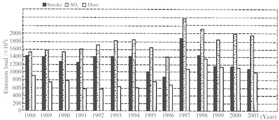
Situation of emission of main pollutants in waste gas between 1988 and 2001

Composition of Atmospheric Dust

The composition and generation amount of atmospheric dust shown in Table 2.3 is the average value within the scope of the world. But for a specific district, especially the industrial city and its close suburb area, the situation is much complex, since the component and quantity varies a lot with different seasons and places.

Inorganic Nonmetallic Particles

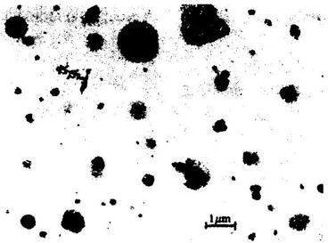
Inorganic particles in atmospheric dust mainly include debris of mineral (including sand), pulverized coal, carbon black, and metal. Figure 2.5 is an electronic microscopic photo of atmospheric dust from a typical industrial city in winter [11]. It is mainly composed of sand, carbon black and crystalline solid material, and a small amount of fiber. In the picture, the silk flocculent particles are coal particles produced by the incomplete combustion of fuels including coal and oil.

Fig. 2.5.

Electronic microscopic photo of atmospheric dust in industrial city.

Upper: observed in general situation; Down: observed by exposure with strong electron beam

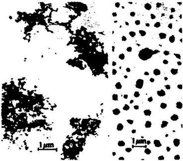
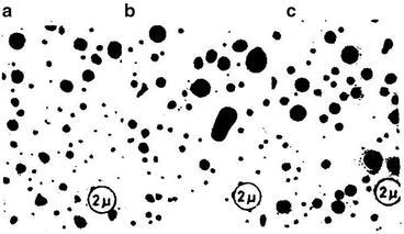
For the atmospheric dust in the suburb, silk flocculent particles are very few, because pulverized coal and carbon black particles by incomplete combustion from exhaust gas of the chimney and automobile are few. This can be seen from the comparison between the left and right cases in Fig. 2.6 [12]. Both Figs. 2.7 and 2.8 also reflect the silk flocculent shape of coal or carbon black particles by incomplete combustion [12]. This is an important method to identify whether it is industrial atmospheric dust. These particles usually have diameter between 0.01 and 1 μm. Figure 2.9 is the local amplification of this shape [13].

Fig. 2.6.

Atmospheric dust in the city (left) and suburb (right)

Fig. 2.7.

Particles generated by combustion of heavy oil (Left: incomplete combustion; Right: complete combustion)

Fig. 2.8.

Particles emitted from automobile

Fig. 2.9.

Microscopic photo of pulverized coal particles (0.01–1 μm). (a) Coal dust particle (amplification ratio 86). (b) Edge of coal dust particle (amplification ratio 860). (c) Edge of black carbon particles (amplification ratio 8,600). (d) Re-amplification for (c) (amplification ratio 860,000)

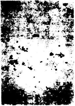
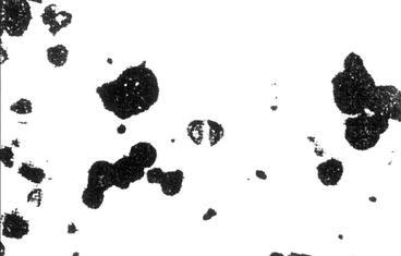
Characteristic of atmospheric dust is different in the city with serious pollution where smog is usually produced by photochemical reaction. In this situation, particles are big in general and most of them are colloidal substances. With strong irradiation of electron beam, most of them will evaporate and only a small amount of solid particles are left. Figure 2.10 is the photo of this kind of atmospheric dust, which looks quite transparent. This is different from the case where pollution is not serious and there is no photochemical smog. In Fig. 2.5, the difference with and without irradiation by electron beam is not obviously seen.

Fig. 2.10.

Atmospheric dust by photochemical reaction before (upper) and after (down) the irradiation of electron beam

Chemical particles generated by photochemical reaction are the very harmful ingredient in atmospheric dust, which produces severe erosion effect on the common material. Figure 2.11 shows the extent of erosion effect [11]. In Part (a) of the figure, particles are captured onto the carbon membrane, and the shape of the particulate matter remains spherical, which means there is no effect of erosion by carbon. In Part (b) of the figure, particles are captured onto the copper membrane, and it is shown that the erosion effect on the copper membrane is very strong (the white part surrounding the particles). In Part (c) of the figure, particles are captured onto the iron membrane, the erosion effect only occurs near particles, and the trace of flying droplets can be seen.

Fig. 2.11.

Erosion effect of particles by photochemical reaction. (a) Particles captured on carbon membrane. (b) Particles captured on copper membrane. (c) Particles captured on iron membrane

Metal Particle

The component of metal in atmospheric dust is strongly related to the development of industry. These years, the high content of metal especially heavy metal such as lead, cadmium, beryllium, manganese, and titanium is found in industrial developed countries. In the city where special fuel is used, mercury and arsenic are also found in the atmospheric dust. Near the factories manufacturing Fe and Mn elements, the concentrations of Fe and Mn are very high. In the exhaust gas of automobile, lead smelting factory and lead battery factory, lead and zinc are discharged. Beryllium can be found in the atmospheric dust emitted from smelting plant, electric bulbs factory, and nuclear power plant. Figure 2.12 shows the X-ray spectrum of the atmospheric dust in Xinglong district of Hebei Province [14], where various kinds of metal components exist.

Fig. 2.12.

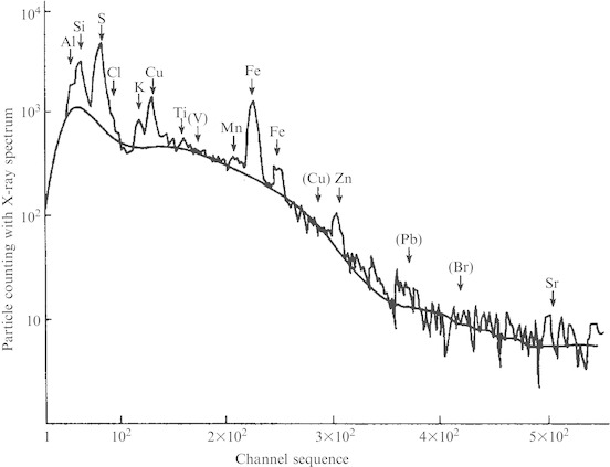
X-ray spectrum of the atmospheric dust

Tables 2.6 [13], 2.7 [15], and 2.8 [16] show the data about the metal component in atmospheric dust of large cities. We can see that in the city where the problem of automobile exhaust pollution is serious, the lead content in atmospheric dust is significantly higher than other element.

Table 2.6.

Metal component of atmospheric dust in Los Angeles, USA

Component	Concentration (μg/m3)	Component	Concentration (μg/m3)	Component	Concentration (μg/m3)
Pb	8.3	Cu	0.45	V	0.034
Mg	8.1	Mn	0.19	As	0.01
Fe	6.2	Ti	0.19	Ag	<0.001
Na	4.2	Sn	0.08	Be	0.
K	3.9	Sr	0.09

Table 2.7.

Metal component of atmospheric dust in Guangzhou

Component	Concentration (μg/m3)
	1	2	3	4	5	6
Cu	0.25	0.12	0.18	0.13	0.14	0.17
Zn	0.18	0.26	0.55	0.088	0.87	0.18
Pb	0.16	0.11	0.18	0.16	0.074	0.025
Mg	0.091	0.11	0.075	0.079	0.060	0.17
Sn	0.075	0.0092	0.017	0.018	0.013	0.0076
Mn	0.43	0.018	0.026	0.071	0.015	0.019
Sb	0.0054	0.0026	0.0037	0.0026	0.0031	0.0017
Cd	0.0051	0.0018	0.0031	0.0024	0.0020	<0.0013
Cr	0.0026	0.0014	0.0026	0.0013	0.0010	0.0023
Bi	0.0019	0.0055	0.0075	0.0013	0.0038	0.000042
V	0.0018	0.00067	0.00060	0.0010	0.00038	0.00090
Ag	0.0010	0.00092	0.0011	0.0013	0.0047	0.00012
Be	0.00075	0.3	0.7	0.00018	0.00015	0.00013

Table 2.8.

Comparison of metal components of atmospheric dust in different cities (μg/m³)

Element	Shanghai	Beijing	Tianjin	Chongqing	Lanzhou (winter)
Ni	0.0457	0.0097	0.0238	–	–
Mn	0.5614	0.1468	0.1994	0.135	0.3696
Fe	8.7309	4.3008	7.1549	3.51	7.9685
Pb	0.4772	0.2429	0.2436	0.36	0.4731
Cd	0.0159	0.0043	0.0045	–	–
Cr	0.0319	0.1524	0.0259	–	–
Cu	0.2056	0.0295	0.0895	0.075	0.1645
Zn	3.3140	0.3585	0.7098	0.36	1.0168
Na	2.7262	0.6408	0.9964	4.85	–
Al	4.4316	8.5446	–	9.6	8.6762
V	0.0188	0.0665	–	–	0.0284

Table 2.9 is the lead content of particles from one measured data [13].

Table 2.9.

Lead content of particles in exhaust gas of automobile

μm	Number	Number percentage (%)	Mass percentage (%)
0–1	724	72.4	6.5
1–2	211	21.1	26.6
2–3	48	4.8	30.4
3–4	12	1.2	22.8
4–5	5	0.5	13.7

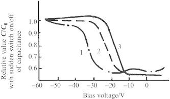
For industrial products, in addition to the harmful effect like usual particles, the particular harmful effect of atmospheric dust especially metal particles is very large. For example, the light metal element Na is very harmful for the semiconductor device. When the quantity of Na polluted at the silicon wafer surface of the semiconductor device is above 3.6 × 10¹¹ atoms/cm², the electrical properties of the device will be affected. Figure 2.13 shows the extent of influence by Na pollution of the surface on the property of integrated circuit [17]. Curve 2 is a pure silicon, and curve 1 is a silicon wafer contaminated by Na. A 70 μm NaCl particle contains the component which has the harmful effect of a single layer of Na pollution on the entire surface of the silicon wafer [18]. Special attention must be paid during the construction of cleanroom factory near ocean. The contribution of NaCl particles in the atmospheric dust in this kind of area reaches 20 %. For example, in the atmospheric dust of the city Qinhuangdao, the component of NaCl in May reaches 2.48–8.01 % (11.18–24.15 μg/m³), while in June it is 14.1–18.9 % (27.19–47.62 μg/m³) [19].

Fig. 2.13.

Influence of Na pollution on the C-U property of integrated circuit

Figure 2.14 is one example of mass distribution of NaCl particles in atmospheric dust [20]. It is shown that most of the seal aerosols in atmospheric dust are within the diameter range near 5 μm in terms of mass. Figure 2.15 presents the particle size distribution of NaCl particles which are generated by atomization with artificial sea water (the mass ratio of NaCl and MgCl₂ is 0.82:0.18) under the relative humidity 60 % [20]. The particle diameter is slightly smaller than that of natural particles.

Fig. 2.14.

Mass distribution of NaCl particles in atmospheric dust

Fig. 2.15.

Mass distribution of NaCl particles by artificial atomizing

The influence of the heavy metal component in the atmospheric dust is much wider. Taking the wafer on the semiconductor device as an example, when the surface concentrations of iron, copper, and silver increased from 10¹¹ to 10¹³ atoms/cm², the effective charge value will change by 2–2.5 times, which is shown in Fig. 2.16 [17]. In this figure, curves 1, 2, and 3 represent the situation with surface concentration of heavy metal 10¹³ atoms/cm², 10¹¹ atoms/cm², and 10⁴ atoms/cm², respectively. Heavy metal is disadvantage for the oscillight of color television. When the fluorescent powder coated on the oscillight is stained by the heavy metal impurities, the light-emitting property of the oscillight will change. This is because the heavy metal penetrating the crystal of the fluorescent powder will become the new energy level center, and it becomes the luminescence center. When the excitation light is located in the range of visible light, the color of fluorescent powder will change. When it is not located in the range of visible light, the brightness will decrease.

Fig. 2.16.

Influence of heavy metal pollution on the C-U property of integrated circuit

Except for the harmful effect for the industrial products, heavy metal particles will cause special hazards for human body. The results are presented in Table 2.10 [21]. Enough attention must be paid on the inorganic particles of the atmospheric dust in city. For example, asbestos are widely used for the materials in the brake, clutch, building materials, and fire insulation, which may cause carcinogenic effect.

Table 2.10.

Hazards of heavy metal component in atmospheric dust for human body

Element	Damaging parts and disease	Concentrations in common cities of UK and USA (μg/m3)
Pb	Nerve, intestines and stomach, anemia	0.2–0.3
Zn	Intestines and stomach, lung, dermatitis	0.004–0.25
Cr	Lung, cancer, dermatitis	0.002–0.02
Co	Lung, heart, dermatitis	0.0007–0.004
Sn	Lung, liver, nerve, dermatitis	0.01–0.03
Ti	Lung, dermatitis	0.01–1.0
Cu	Dermatitis	0.02–0.9
Ni	Nerve, lung, cancer, dermatitis	0.002–0.2
V	Lung, dermatitis	0.001–0.1
As	Lung, nerve, liver, kidney, intestines, skin caner	0.01–0.02
Be	Lung, dermatitis	0.0001–0.001
Mn	Lung, nerve	0.01–0.3
Mo	Nerve, anemia, maldevelopment	0.0005–0.006

Organic Particle

Natural organic particles in atmospheric dust mainly include plant pollen, fiber, animal hair, dander, and excretion. In the area of cotton and textile industry, the concentration of cotton fiber in atmospheric dust is significantly higher than that of other areas. More organic particles are generated by artificial means, including hydrocarbons and tiny plastic particles emitted from various pollution sources.

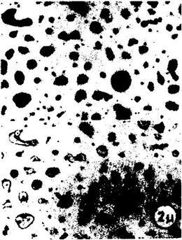
Here the information about pollen will be emphasized. During the season of pollen outbreak, it will generate many particles between 10 thousands and 1 million. In average it will be several hundreds of thousands. Figure 2.17 shows the situation of atmospheric dust containing the pollen in city [22]. The concentration of pollen in atmospheric dust is related to season. It is shown in Fig. 2.18 that the amount of pollen generated in the period between the spring and summer is the largest [22]. Pollen particles are usually large with semi-monodisperse distribution. Figure 2.19 shows the photo of pollen [22]. Therefore, there is requirement for the variety of tree during the design of afforest scheme for cleanroom factory. These trees with quick effect of afforest, less pollen generation, and no floral production should be chosen.

Fig. 2.17.

Pollen in the atmospheric dust (the pollen is located in the middle)

Fig. 2.18.

Example of pollen concentration in city

Fig. 2.19.

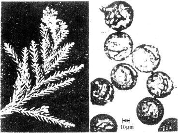
Firry pollen (30 μm)

Vital Particle

In atmospheric dust, there are also a small proportion of vital particles, i.e., microorganism, including protozoa, unicellular algae, fungi, bacteria, rickettsia, and viruses. Among the bacteria, there are also 20 kinds of coccus, 8 kinds of staphylococcus aureus, 37 kinds of tuberculosis, and 7 kinds of blastomycosis. Except for the larger protozoa and unicellular algae, there are other kind of microorganisms existing, which has four types of basic state including fungal spores, bacteria bacillus, cenobium (propagant), and virus.

Illustration will be presented later about the features of vital particles.

Composition of Atmospheric Dust

In general, the composition of atmospheric dust in and near city is shown in Table 2.11.

Table 2.11.

Composition of atmospheric dust

Composition	Content (%)
Mineral debris, dross from combustion	10–90
Smoke and pollen	0–20
Plant fiber such as cotton	5–40
Fine particles including coal, charcoal, cement, and concrete	0–40
Decayed plant, scurf	0–10
Metal	0–0.5
Microorganism	Extreme small

Concentration of Atmospheric Dust

Methods to Express Concentrations

There are three methods to express the concentrations of atmospheric dust:

1. Particle counting concentration. Particle number in unit volume of air, expressed with pc/L

2. Gravimetric concentration. Particle mass in unit volume of air, expressed with mg/m³

3. Settlement concentration. Number or mass of particles deposited naturally onto the surface with unit area within unit time, expressed with pc/(cm²∙h) or t/(km²∙month)

Large variation exists for the concentration of atmospheric dust. In order to determine the concentration of atmospheric dust in a scientific way, we should distinguish the instantaneous (for one time) value from the mean value, or the maximum from minimum value. Or the average, maximum and minimum values should be provided at the same time. As for the average value, the difference between 1 h average, 24 h (1 day) average, and month average must be distinguished. The longer the time is, the smaller the average value is. It is necessary to indicate the continuous average time, such as 1 h mean value with continuous 48 h sampling, or with 8 h sampling every day, and so on. As for the minimum and maximum value, the information about the time for sampling is also needed, such as the daily maximum (minimum) value.

From the environment and health, industrial hygiene, and general air-conditioning point of view, gravimetric concentration and settlement concentration are used to describe the concentration of atmospheric dust. In the field of air cleaning technology, the particle counting concentration of atmospheric dust is adopted, but the gravimetric concentration also has the value for reference, such as in the calculation process of particle loading in air filters.

Background Value of Atmospheric Dust Concentration

Generally, concentration of atmospheric dust located 2 km above the ground can be regarded as the background value, which is shown in Table 2.12.

Table 2.12.

Background value of atmospheric dust concentration (pc/L)

Place	Full size	Above 0.5 μm	Above 0.3 μm	Above 5 μm	Pollen	Virus	Bacterium	Mould	Spore
Ocean	210,000	2,500	7,500	28	–	–	–	–	–
Stratosphere
10 km	35,000	20	55	–	0.1	–	(0.5–100) × 10−3	0.1–10	0–100

Gravimetric Concentration

The determination of gravimetric concentration of atmospheric dust is based on the influence on occupant’s health, especially the influence on the respiratory system. The situation of particle penetration and deposition depth in respiratory system is shown in Table 2.13 [23] and Fig. 2.20 [24].

Table 2.13.

The relationship between particle size and deposition depth in respiratory system

Particle size (μm)	Reachable sites
30	Arrive at the trachea of the back, not above the branch part
10	Arrive at terminal bronchi
3	Arrive at alveolar way
1	Most deposit in the alveolar way and alveolar sac (2.6 % exhaled again)
0.3	Most deposit in the alveolar sac (65 % exhaled again)
0.1	Most deposit in the alveolar sac (65 % exhaled again)
0.03	Most deposit in the alveolar way and alveolar sac (34 % exhaled again)

Fig. 2.20.

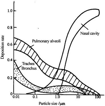
Deposition rate of particles onto human respiratory system with the particle size

Four principles should be considered to study the influence on human:

The Influence Extent on Health

The influence extent of the variation of gravimetric concentration on occupant’s health should be determined according to the statistical material, which is the paramount principle.

The death event caused by the famous British London fog shows vividly the relationship between gravimetric concentration of atmospheric dust and mortality rate, which is shown in Fig. 2.21 [13]. It can be seen that when the weigh concentration is above 0.2–0.25 mg/m³, it is not a general problem, but is related to death apparently.

Fig. 2.21.

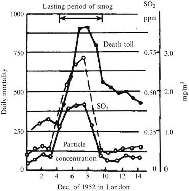
Relationship between atmospheric dust concentration and the mortality rate

Table 2.14 is the trend of influence by the variation of gravimetric concentration of atmospheric dust on human health based on the statistical investigation from some countries. It is shown that when the averaged value is obtained with 24 h every day, the concentration limit of death is 0.15 mg/m³.

Table 2.14.

Effect of atmospheric dust on human health

Concentration (μg/m3)	Influence
100 (24 h average annually)	Diseases such as chronic bronchitis increase, children asthma
150 (24 h average)	Increased death for patients, infirm, old man
300 (1 h average)	Visual distance less than 8 km, with flight difficulties, increased mortality
600 (1 h average)	Visual distance less than 2 km, traffic accident, illness, and increased mortality
From 140 to 60 (average)	The sputum generated will drop accordingly

Since the beginning of 1990s, due to the study of epidemic, requirement was put forward for particles with aerodynamic diameter ≤2.5 μm (expressed as PM_2.5). The national Environmental Protection Agency (EPA) of America modified the particle index from the original total suspended particles (TSP) to particles with aerodynamic diameter ≤10 μm (expressed as PM₁₀). Later in the revised Ambient Air Quality Standard, the upper limit for PM_2.5 was specified. According to the definition of the aerodynamic diameter (shown in Eq. (10.1007/978-3-642-39374-7_1)), the real diameter for particles with density larger than 1 is smaller than 2.5 μm, while it is larger than 2.5 μm for those with density less than 1.

Self-Feeling of Pollution by Occupants

Based on the experimental survey for a certain amount of population, the relationship between the feeling of pollution and the gravimetric concentration is established. One example is shown in Table 2.15 [25]. It is shown that most people will have the feeling for the existence of pollution when the gravimetric concentration is more than 0.15 mg/m³. This is why many countries set 0.15 mg/m³ as atmospheric pollution concentration limit for the hygiene standard and design standard.

Table 2.15.

Investigation of the pollution concentration

Pollution condition	Proportion
	Dust content 0.1–0.15 mg/m3	Dust content 0.23–0.38 mg/m3
Feeling the existence of pollution	10 %	90 %
No feeling the existence of pollution	90 %	10 %

The World Health Organization (WHO) recommended the annual average concentration of total suspended particulate less than 0.06–0.09 mg/m³ and the daily average concentration less than 0.15–0.23 mg/m³, according to statistical data of all countries [8].

Degree of No Guarantee

The design standard of gravimetric concentration is determined with the degree of no guarantee (also termed as risk probability) of gravimetric concentration according to the factors including experience and techniques.

In a region, dozens or even hundreds of representative points can be selected. Measurement will be taken at each point every hour. In total 8,760 data will be obtained 1 year. The cumulative distribution curve of gravimetric concentration can be plotted. Then the value of gravimetric concentration with the expected degree of no guarantee can be determined. The so-called degree of no guarantee means how many monthly or daily average concentration in a year surpass this expected gravimetric concentration, which is used as the basis for the design standard. For example, when the degree of no guarantee for residential area of America is set 5 %, the daily average value in a year becomes 0.15 mg/m³. The degree of no guarantee is dependent on the necessity, economic, and technical conditions. For example, the degree of no guarantee for extreme strict application and allowable economical condition can be 2.5 %. The gravimetric concentration corresponding to the degree of no guarantee should be determined with the actual conditions. For example, in the corresponding concentration with the proposed degree of no guarantee in 1986, Japan was lower by 10–23 % than that of 1975, which is shown in Table 2.16 [26]. This is because the concentration of atmospheric dust generally reduced with the improvement of the environment.

Table 2.16.

Change of suggested gravimetric concentration in Tokyo area

Grade	Measured results in Tokyo (mg/m3)		The recommended design value (mg/m3)				Corresponding environment
			No assurance 2.5 %		No assurance 5 %
	No assurance 2.5 %	No assurance 5 %	1975	1986	1975	1986
1	−0.13	−0.09	0.16	0.13	0.13	0.10	Suburbs with fresh air
2	0.13–0.15	0.09–0.11	0.19	0.16	0.15	0.12	Suburbs
3	0.15–0.17	0.11–0.13	0.22	0.19	0.17	0.14	Commercial residential
4	0.17–0.19	0.13–0.15	0.25	0.22	0.19	0.16	Commercial street
5	0.19–	0.15–	0.28	0.25	0.21	0.18	Urban with serious air pollution

Magnitude of Particle Size

The abovementioned atmospheric dust means the total suspended particle (TSP), while particulate matter (PM) is a term in environmental science. Usually particles with aerodynamic diameter between 2.5 and 10 μm are called coarse particles. Those between 0.1 and 2.5 μm are called fine particles. Those less than 0.1 μm are called ultrafine particles. In this book, all of them are called particles.

With the further investigation of epidemic, the standards about gravimetric concentration for atmospheric dust in many countries are more related to the magnitude of particles, which proves the saying “it will be a trend” in the past version of this book.

Ultrafine particles (UF), i.e., particles with diameter smaller than 0.1 μm, have attracted the attention of scientific community. However, the current investigation results of epidemic do not provide enough proof about the relationship between exposure and reaction. This is why the concentration of UF with the expression of particle counting concentration does not become the aim of air quality standard.

Since PM₁₀ represents those particles which are able to enter the respiratory tract, it becomes the index of particles for studying the exposure of people in the past time. Therefore, the concentration of PM₁₀ is monitored in most common air quality monitoring system.

According to the “Air Quality Guideline” published by WHO in 2006, when the short-term exposure concentration of PM₁₀ increases by 10 μg/m³ (24 h averaged), the mortality rate will increase by 0.46 % or 0.62 %. When the concentration of PM₁₀ reaches 150 μg/m³, the mortality rate is expected to increase by 5 %.

In 1987, Environmental Protection Agency (EPA) of the USA adopted PM₁₀, i.e., these particles with aerodynamic diameter ≤10 μm, as the index for particles, instead of the total suspension particles (TSP).

In 1982, Chinese national standard “Ambient Air Quality Standard” (GB3095-82) adopted the TSP as the index. In the revised version in 1996 (GB3095), PM₁₀ was adopted, and ambient air was defined as the outdoor air exposed by people, plant, animal, and building.

However, study has shown that organic material plays a role in the influence of particles on health. In atmospheric dust, organic material is inclined to exist in fine particles. Fine particles are likely to absorb heavy metal, acid oxidant, and organic pollutants in the air. Table 2.17 shows the absorbed elements [27].

Table 2.17.

Distribution of various elements in particles with different sizes

Element	June			December
	PM2.5	PM2.5–10	PM10–100	PM2.5	PM2.5–10	PM10–100
K	55.22	20.34	24.43	43.39	12.62	43.99
Na	59.27	36.19	4.54	50.01	20.12	29.87
Ag	57.68	36.62	5.70	–	–	–
Al	39.58	44.54	15.88	36.19	32.99	30.82
As	57.70	41.18	1.12	41.77	20.70	37.53
Ba	29.70	34.59	35.72	53.02	29.68	17.30
Ca	28.85	42.71	28.44	34.80	32.98	32.22
Co	56.55	39.35	4.10	79.00	2.86	18.14
Cr	22.52	60.38	17.10	56.10	41.45	2.45
Cu	30.53	23.51	45.96	61.99	36.99	1.02
Fe	32.28	36.62	31.11	41.76	41.11	17.13
Mg	45.90	41.21	12.89	44.34	42.91	12.75
Mn	33.58	17.42	48.99	54.99	21.66	23.35
Ni	86.51	1.08	12.41	80.53	15.43	4.04
P	39.71	26.44	33.86	53.29	21.13	25.58
Pb	62.65	22.73	14.62	54.19	14.93	30.88
S	77.28	13.41	9.31	49.97	14.85	37.18
Se	60.90	26.79	12.31	38.31	16.41	45.28
Sn	91.03	8.18	0.79	44.37	52.07	3.55
Ti	44.16	42.34	13.50	41.18	18.62	40.20
V	62.31	35.71	1.98	42.70	13.67	43.64
Zn	58.50	13.20	28.30	66.73	23.05	10.22
Average	51.47	30.21	18.32	49.38	27.49	23.13

Research results have shown that the lower limit of concentration influencing the survival rate significantly is 10 μg/m³, such as American Cancer Society (ACS). Some former studies have also shown the strong correlation between long exposure to PM_2.5 and the mortality rate. This resulted in the modification of Ambient Air Quality Standard in the USA in 1997, which specified the upper limit of PM_2.5.

Revisions and drafts have been made for the “Air Quality Guideline” published by WHO in 1987, 1997, and 2005, respectively. After that, it recommended to choose PM_2.5 as the prior index for particles.

In 2012, the Chinese standard “Ambient Air Quality Standard” was revised, which will be implemented. Both PM₁₀ and PM_2.5 are included in this standard.

Study has shown that when the daily averaged concentration of PM_2.5 increases by 10 μg/m³, the total mortality rate will increase by 1.5 % [28]. The mortality rate of stubborn pulmonary disease will increase by 3.3 %, and that of local blood scarce heart disease will increase by 2.1 %. There are other reports showing that the daily total mortality rate will increase by 10 %, the respiratory system disease increased by 3.4 %, cardiovascular disease increased by 1.4 %, asthma increased by 3 %, and lung function decreased by 0.1 % [29]. International Standard Organization (ISO) proposed to consider particles with diameter less than 2.4 μm as the “high-risk particle” to induce the lung disease for children and adult [30], which is equivalent with PM_2.5.

Study has shown that the poisonous mechanisms of PM_2.5 mainly include [29]:

1. Immune toxicity. Not only the nonspecific immunity function of macrophagocyte is affected, but also the immune performance of cell with specific immunity function is damaged.

2. Oxidation damage toxicity. Except for the radical reactivity itself, particles can also have effect on the epithelial cell and the macrophagocyte. The active oxygen or active nitrogen will be released, and the polyunsaturated fatty acids abundant on the membrane of cell will be oxidized, which will influence the permeability and the mobility of the membrane. The structure of the membrane will be thus damaged.

3. Mutagenicity and potential carcinogenic effect. Toxic heavy metal and PAH (polycyclic aromatic hydrocarbon) absorbed on particles have strong ability of mutagenicity, which can cause the cell division, cultivate the tumor, and have the potential carcinogenic effect.

However, these conclusions have also received accusation from enterprises who believed that it is likely to be overstated. But in other aspect, it is believed that the particles with harmful effect are smaller. For example, the relevant domestic research [31] points out that about 50–70 % of polycyclic aromatic hydrocarbon and 30–50 % of N-alkane are absorbed to particles with diameter ≤0.1 μm. It is shown from Fig. 2.20 that this kind of particles has the health significance, which can penetrate through and deposit onto the trachea, bronchus, and especially alveoli. In this sense, the following conclusions can be obtained: since the annual concentration of atmospheric dust for particles with diameter ≤0.1 μm (measured with the 6th layer of cascade impactor, i.e., Anderson sampler) in the winter of Guangzhou is 1.6 times than that in Beijing, and in summer the ratio between two cities becomes 1.8 times (shown in Fig. 2.22), the atmosphere with the same concentration of atmospheric dust in Guangzhou is more harmful than that in Beijing.

Fig. 2.22.

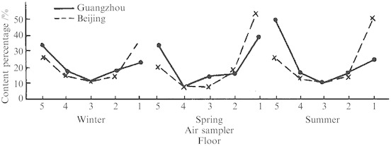
Comparison of mass percentage for particles between Guangzhou and Beijing

In the above section, the change of gravimetric concentration standard was discussed. Next the transition of specific standards is presented.

In the “Ambient Air Quality Standard” published in 1982, air quality is classified into three categories:

• The first class aims to protect the natural ecology and human health. With the long term of exposure, the air will not cause any risk of harmful effect.

• The second class aims to protect the human health, animal, and plant in both urban and rural areas. With the long and short term of exposure, the air will not cause a harmful effect.

• The third class aims to protect the human from acute and chronic poisoning and to protect the normal growth of the common animal and plant in city (except the sensitive one).

In this standard, the first class area includes the national specified natural reserves, scenic tourist area, scenic spots and historical resort, and salutarium, where the air with the first class applies. In the revised version of 1996, the salutarium is deleted and replaced by special reserve. The second area includes the city planning specified residential area, the mixed area of commerce, traffic and residence, the cultural area, scenic spots and historical sites, and rural area, where the air with the second class applies. In the revised version of 1996, the general industrial area in the former third class area is classified into the second class area. The third class area includes the city and town with serious air pollution, as well as the industrial area, where the air with the third class applies. In the revised version of 1996, the “urban transportation hub and city” area in the former third class area is deleted. In the revised version of 2012, the third class area is merged into the second class area, and the concentration of PM_2.5 is required.

It should be noted that there are several kinds of average concentration:

• Yearly averaged concentration: The arithmetic average of daily averaged concentrations within any 1 year period.

• Quarterly averaged concentration: The arithmetic average of daily averaged concentrations within any one quarter period, which is mainly useful for the lead.

• Monthly averaged concentration: The arithmetic average of daily averaged concentrations in 1 month, which is abolished in the 2012 version.

• Daily averaged concentration: The average concentration in 1 day, which is abolished in the 2012 version.

• 24 h averaged concentration: The arithmetic average of hourly averaged concentrations within 24 h of 1 day, which is also called daily averaged concentration (adopted in the 2012 version).

• 1 h averaged concentration: The arithmetic average of concentrations in 1 h.

Moreover, there are also other kinds which include 8 h averaged concentration and growth season averaged concentration (mainly for fluoride).

Table 2.18 illustrates the change of standards for atmospheric dust concentration in China, and the comparison with American standard is also presented. Table 2.19 shows the target value of WHO.

Table 2.18.

Ambient Air Quality Standards in China and America

Nationality	Standard development department	Particle concentration (μg/m3)						Allowable time with concentration larger than the limit	Remark
			Annual average	Daily average	1 h average	Limit	Average time
America	National standard for air quality in 1971	Class I		0.260				99.7 % in 1 year
		Class II		0.150				99.7 % in 1 year
		Country		0.13				95 % in 1 year
		Residential district		0.15				95 % in 1 year
		Industrial area		0.2				95% in 1 year
	In 1987 (PM10)	Class I	0.050	0.150
	In 1997 (PM2.5)		0.015	0.065				Three consecutive years with concentration not less than 98 % of the average daily concentration
China	National standard “Ambient Air Quality Standard” (GB3095-82) issued in 1982 and the revised edition in 1994	Total suspended particles
		Level 1	0.10	0.15
				(0.15)		(0.30)	(Any time)		Value in () is from the standard in 1982
		Level 2	0.20	0.30
				(0.30)		(1.00)	(Any time)		Value in () is from the standard in 1982
		Level 3	0.30	0.50
				(0.50)		(1.50)	(Any time)		Value in () is from the standard in 1982
		Inhalable particles
		Level 1	0.04	0.05
				(0.05)		(0.15)	(Any time)		Value in () is from the standard in 1982
		Level 2	0.10	0.15
				(0.15)		(0.50)	(Any time)		Value in () is from the standard in 1982
		Level 3	0.15	0.25
				(0.25)		(0.70)	(Any time)		Value in () is from the standard in 1982
	Revised standard “Ambient Air Quality Standard” in 2012 (implemented in Jan. of 2016)	PM10							In the standard, the unit has been changed from mg/m3 into μg/m3
		Level 1	0.04	0.05
		Level 2	0.07	0.15
		PM2.5
		Level 1	0.015	0.035
		Level 2	0.035	0.075

Table 2.19.

Air Quality Guideline (AQG) value in WHO and some countries: annual averaged concentration/24 h concentration

	PM10 (μg/m3)	PM2.5 (μg/m3)
WHO: target during transient period-1(IT-1)	70/50	35/75
Target during transient period-2(IT-2)	50/100	25/50
Target during transient period-3(IT-3)	30/75	15/37.5
Air quality guideline (AQG) value	20/50	10/25
USA (implemented on Dec.17, 2006)		15/35
Japan (issued on Sept. 9, 2009)		15/35
EU (issued on Jan. 1, 2010, implemented on Jan. 1, 2015)		25/None

From the world, the gravimetric concentration of atmospheric dust declines year by year. According to the survey data of 37 countries by the US Environmental Protection Agency, concentration of atmospheric dust in 19 cities declines, that of 12 cities remains the same, and only that of 6 cities increases [8]. The most seriously polluted cities with concentration larger than the recommended value by WHO include Beijing, Calcutta, New Delhi, and Xi’an.

But as for the specific situation in China, the ambient air is seriously polluted, which is shown in Table 2.20 [32]. Table 2.21 is the sorting sequence of atmospheric dust concentrations in several cities in 2000. Table 2.22 is the sorting sequence of particle deposition [32]. It is clear that northern concentration is obviously larger than that of the southern region. However, the atmospheric dust concentration is decreasing, which can be found in Table 2.23 with the sorted data by author according to “China Environment Yearbook.” The trendy is also presented in Fig. 2.23, where the data from Taiwan and Japan are also included [26, 33]. The concentration data in China is higher than that of Japan. The good news is that, since 1997, the annual average concentration has been less than the third class, and the trend is continuing to decrease. The peak situation of the dust emission for whole nation shown in Fig. 2.4 is not reflected here. One situation must be noticed that the emission quantity of industrial dust and smoke for the whole nation in 1997 is less than that of 1996, according to the “China Environment Yearbook” published in 1998. The emission quantity in 1997 is far less than that of 1998, which is less than 85 % of the total emission quantity for the whole nation. When other factors are also considered, the total suspended particles are resulted to decrease.

Table 2.20.

Situation of over-standard concentration for atmospheric dust from 1981 to 1990

Overweight situation	Seriously affected area
100 % of particle concentrations in the air of northern cities exceed the standard value, and near 100 % of southern cities are overweight	Hohhot, Taiyuan, Jinan, Shijiazhuang, Lanzhou, Qinhuangdao, Beijing, Tianjin, Chongqing, Shenyang
The pollution of falling dust is very serious regardless of north and south, almost 100 % cities are overweight	Baotou, Benxi, Taiyuan, Shijiazhuang, Anshan, Changchun, Harbin, Shenyang, Urumqi, Jinan

Table 2.21.

Sorting sequence of annual average concentration of total suspended particles in national monitoring cities in 2000 (mg/m³)

Northern city	Annual average concentration	Southern city	Annual average concentration
Datong	0.721	Chengdu	0.435
Lanzhou	0.668	Zigong	0.310
Golmud	0.563	Yibin	0.290
Jilin	0.557	Jiujiang	0.268
Yan’an	0.545	Lhasa	0.266
Urumqi	0.501	Nanchong	0.263
Jiaozuo	0.498	Chongqing	0.261
Anyang	0.496	Pingxiang	0.254
Hohhot	0.451	Wuhan	0.253
Xining	0.433	Xiangfan	0.252
Shijiazhuang	0.431	Zhuzhou	0.250
Anshan	0.418	Yichang	0.244
Taiyuan	0.401	Hechi	0.225
Pingdingshan	0.398	Sanming	0.213
Baotou	0.380	Liupanshui	0.211
Shizuishan	0.379	Hengyang	0.201
Baoji	0.365	Guiyang	0.209
Baoding	0.362	Chengdu	0.198
Luoyang	0.354	Guangzhou	0.185
Beijing	0.353	Nanchang	0.180
Tangshan	0.352	Jingdezhen	0.180
Xian	0.351	Changsha	0.179
Yinchuan	0.342	Huaihua	0.172
Hami	0.325	Hefei	0.170
Xuzhou	0.323	Baise	0.167
Kaifeng	0.320	Leshan	0.165
Tianjin	0.304	Nanning	0.162
Zhengzhou	0.291	Gejiu	0.161
Tumen	0.290	Wuzhou	0.161
Qinhuangdao	0.283	Shanghai	0.156
Hegang	0.279	Ningbo	0.154
Qitaihe	0.271	Kunming	0.152
Changchun	0.265	Suzhou	0.152
Shenyang	0.265	Wenzhou	0.149
Siping	0.245	Hangzhou	0.141
Harbin	0.242	Guilin	0.139
Hailar	0.238	Anqing	0.119
Hanzhong	0.238	Zhuhai	0.119
Zibo	0.219	Ganzhou	0.116
Huludao	0.218	Fuzhou	0.113
Yuncheng	0.216	Nantong	0.108
Lianyungang	0.179	Nanjing	0.107
Jinan	0.173	Zhanjiang	0.093
Yichun	0.154	Shenzhen	0.091
Qingdao	0.143	Xiamen	0.084
Ji’an	0.139	Haikou	0.077
Daqing	0.118
Dalian	0.088
Average in north	0.336	Average in south	0.186

Table 2.22.

Sorting sequence of average annual quantity of dustfalls in national monitoring cities in 2000 (t/(km² ∙ month))

Northern city	Dustfall	Southern city	Dustfall
Baoding	38.4	Zhuzhou	27.8
Datong	35.5	Lhasa	20.4
Anshan	35.3	Wuhan	14.1
Yinchuan	35.2	Changsha	13.5
Qitaihe	28.3	Guiyang	13.3
Jiaozuo	28.1	Hangzhou	13.1
Xi’an	27	Xiangfan	11.8
Urumqi	26.9	Nanchong	11.7
Hegang	25.5	Chongqing	11.5
Luoyang	25.4	Chengdu	11.3
Siping	25	Liupanshui	11.1
Jilin	25	Yibin	11
Shijiazhuang	23	Nanjing	10.9
Shizuishan	21.6	Yichang	10.2
Kaifeng	21.4	Jiujiang	9.8
Hailaer	21.4	Nanchang	9.8
Shenyang	21.3	Hengyang	9.7
Lanzhou	21.1	Shanghai	8.9
Xining	19.7	Guilin	8.4
Anyang	19.3	Zigong	8.4
Jinan	18	Wenzhou	8.2
Tangshan	17.7	Anqing	8.2
Zibo	17.3	Nantong	8.1
Dalian	17.2	Kunming	7.4
Qingdao	17.1	Guangzhou	7.3
Harbin	17	Fuzhou	7.1
Zhengzhou	17	Hefei	6.8
Pingdingshan	15.9	Suzhou	6.8
Baoji	15.6	Leshan	6.7
Hami	15.4	Nanning	6.5
Tianjin	15.4	Pingxiang	6.4
Changchun	15.2	Hechi	6
Beijing	15.1	Jingdezhen	5.9
Yan’an	14.8	Ganzhou	5.8
Tumen	13.9	Wuzhou	5.5
Daqing	13.5	Gejiu	5.4
Hohhot	13.4	Ningbo	5.4
Qinghuangdao	13	Xiamen	5.2
Xuzhou	12.1	Huaihua	5.1
Yichun	12	Shenzhen	5
Hanzhong	8.9	Baise	4.5
Huludao	7.3	Zhanjiang	4.4
Lianyungang	7.3	Haikou	3.2
Ji’an	5.6	Zhuhai	2.6
Average in north	19.5	Average in south	8.8

Table 2.23.

Comparison between the particulates and the dustfall

Item	Year	Whole country		Southern cities		Northern cities
		Concentration rage	Annual average	Concentration rage	Annual average	Concentration rage	Annual average
Particle (mg/m3)	1981	0.160–2.770	0.703	0.160–0.850	0.41	0.370–2.770	0.93
	1982	0.220–1.910	0.729	0.220–0.970	0.47	0.380–1.910	0.95
	1983	0.164–1.358	0.6	0.164–0.540	0.33	0.427–1.358	0.87
	1984	0.190–2.158	0.66	0.190–1.030	0.45	0.370–2.158	0.87
	1985	0.224–1.767	0.59	0.224–0.821	0.444	0.333–1.767	0.74
	1986	0.196–1.575	0.57	0.219–0.627	0.391	0.196–1.575	0.715
	1987	0.154–1.357	0.59	0.154–0.573	0.37	0.439–1.357	0.805
	1988	0.220–1.597	0.58	0.220–0.740	0.44	0.270–1.597	0.674
	1989	0.117–1.043	0.432	0.141–0.916	0.318	0.117–1.043	0.526
	1990	0.064–0.844	0.379	0.064–0.800	0.268	0.138–0.844	0.475
	1991	0.080–1.433	0.324	0.080–0.376	0.225	0.709–1.433	0.429
	1992	0.090–0.063	0.323	0.090–0.474	0.25	0.134–0.663	0.4
	1993	0.108–0.815	0.327	0.108–0.721	0.252	0.142–0.815	0.406
	1994	0.089–0.849	0.316	–	0.25	–	0.407
	1995	0.055–0.732	0.317	–	0.242	–	0.392
	1996	0.079–0.618	0.309	–	0.23	–	0.387
	1997	0.032 ~ 0.741	0.291	–	0.2	–	0.381
	1998	0.011–1.199	0.289	–	0.199	–	0.364
	1999	–	0.266	–	0.179	–	0.346
	2000	–	0.264	–	0.186	–	0.336
Dustfall [t/(km2 · month)]	1981	10.79–103.75	35.35	10.79–46.50	18.76	21.42–103.75	50.67
	1982	10.83–99.73	32.08	10.83–35.69	16.69	23.73–99.73	48.76
	1983	5.10 ~ 113.90	32	5.10–29.70	16	19.90–113.90	48
	1984	4.048–87.60	27.2	4.48–43.14	16.1	15.30–87.61	38
	1985	7.53–76.50	27.65	7.53–43.69	16.5	16.04–76.50	38.81
	1986	5.96–68.57	25.02	5.96–29.45	13.22	14.82–68.57	32.58
	1987	7.53–73.97	24.41	7.53–26.13	14.09	14.27–73.97	32.79
	1988	7.04–131.25	25	7.04–69.00	13.5	9.90–131.25	35
	1989	3.77–56.70	22.37	3.77–61.92	15.27	6.78–54.61	27.7
	1990	3.22–51.17	19.15	3.71–17.27	10.6	5.91–56.70	26.05
	1991	3.22–51.17	18.1	3.22–49.75	11.05	7.38–51.17	25.46
	1992	3.84–55.75	18.8	3.84–55.75	12.05	9.90–51.08	26.25
	1993	4.03–83.47	18.84	4.03–19.85	10.11	8.50–83.47	26.64
	1994	–	17.6	–	10.57	–	24.76
	1995	–	17.7	–	10.16	–	24.73
	1996	–	16.2	–	9.14	–	23.2
	1997	–	15.3	–	9.29	–	21.48
	1998	–	15.15	–	8.84	–	21.06
	1999	–	14.3	–	8.5	–	20.1
	2000	–	14.15	–	8.8	–	19.5

Fig. 2.23.

Change of urban atmospheric dust for 10 years at home and abroad. (a) Total suspended particulates in China. (b) Deposition particulates in China. (c) Total suspended particulates in Taiwan. (d) Atmospheric dust in Tokyo area of Japan

Since 2004, the concentration of TSP by artificial measurement method is no longer reported, and the concentration of PM₁₀ by automatic measurement method is adopted. Therefore, the data about TSP is still kept till the end of 2000, but it is impossible to compare these data with the following data. Table 2.24 shows the reported concentration of TSP in some cities for the last time, which is very previous. This is why it is cited here for reference [34].

Table 2.24.

Concentration of TSP in some cities in 2004

Northern cities	Annual average	Southern cities	Annual average
Hetian	1.424	Lhasa	0.267
Aksu	0.817	Liuzhou	0.227
Kashgar	0.806	Liupanshui	0.201
Wuhai	0.564	Tongren	0.200
Artux	0.550	Hechi	0.199
Turpan	0.508	Chengdu	0.199
Korla	0.482	Guigang	0.195
Xining	0.472	Hezhou	0.190
Baiyin	0.451	Baise	0.184
Wuzhong	0.449	Xingyi	0.173
Golmud	0.446	Yingtan	0.168
Zhongwei	0.406	Qinzhou	0.157
Hohhot	0.353	Duyun	0.123
Tianshui	0.329	Anshun	0.122
Yining	0.327	Fangchenggang	0.118
Wuwei	0.322	Kaili	0.116
Linxia	0.312	Chishui	0.101
Liaoyuan	0.301	Wuzhishan	0.014
Dingxi	0.297
Benxi	0.295
Shangluo	0.292
Hami	0.291
Ankang	0.287
Pingliang	0.285
Tongliao	0.284
Jinzhou	0.280
Anyang	0.279
Hezuo	0.274
Zhangye	0.269
Siping	0.262
Kuitun	0.261
Yulin	0.258
Fushun	0.241
Ulanqab	0.234
Qitaihe	0.220
Bole	0.217
Shuangyashan	0.210
Changji	0.209
Jiuquan	0.207
Tacheng	0.200
Liaoyang	0.199
Chaoyang	0.198
Changchun	0.185
Baishan	0.182
Panjin	0.182
Ji’an	0.179
Tumen	0.173
Qiqihar	0.172
Yingkou	0.170
Songyuan	0.167
Dandong	0.166
Yichun	0.136
Baicheng	0.135
Altay	0.110

Unit: mg/m³

According to “Environmental Report of China” [35], PM10 concentration distribution in many provinces and cities in 2010 was presented, which is shown in Fig. 2.24. The primary pollutant in Key environmental protection cities is mainly the respirable particles, which occupies 93.5 %. Figure 2.25 shows the situation of key cities with pollution more than 50 days.

Fig. 2.24.

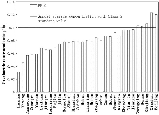
Gravimetric concentration distribution of PM10 in different provinces (autonomous regions and municipalities)

Fig. 2.25.

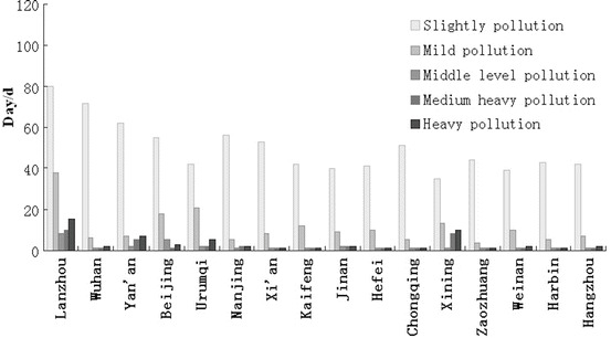
Key cities of environmental protection where the concentration of the primary pollutant PM₁₀ overweight for 50 days

Of course, after the erupt of sand storm, the concentration of PM₁₀ may increase by several times. Figure 2.26 is one example from Beijing [35].

Fig. 2.26.

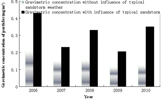
Annual variation of air quality with the influence of the typical sand storm

Table 2.25 mainly shows the annual average concentration of PM₁₀ in cities with the level above the county, but some TSP data are also included for individual cities [35]. They are listed in the corresponding province.

Table 2.25.

Annual average concentration of PM₁₀ in cities with the level above the county in 2010 (mg/m³)

Beijing	0.121	Dandong	0.069	Zhenjiang	0.097	Jingdezhen	0.064	Zhoukou	0.106
Tianjin	0.096	Jinzhou	0.079	Taizhou	0.087	Pingxiang	0.066	Zhumadian	0.094
Hebei		Yingkou	0.073	Suqian	0.099	Jiujiang	0.064	Hubei
Shijiazhuang	0.098	Fuxin	0.094	Zhejiang		Xinyu	0.077	Wuhan	0.108
Tangshan	0.085	Liaoyang	0.066	Hangzhou	0.098	Yingtan	0.058	Huangshi	0.091
Qinghuangdao	0.064	Panjin	0.074	Ningbo	0.096	Ganzhou	0.059	Shiyan	0.081
Handan	0.09	Tieling	0.078	Wenzhou	0.085	Ji’an	0.072	Yichang	0.086
Xingtai	0.082	Chaoyang	0.083	Jiaxing	0.093	Yichun	0.059	Xiangfan	0.089
Baoding	0.084	Huludao	0.076	Huzhou	0.086	Fuzhou	0.057	Ezhou	0.083
Zhangjiakou	0.07	Jilin		Shaoxing	0.095	Shangrao	0.058	Jinmen	0.106
Chengde	0.053	Changchun	0.089	Jinhua	0.067	Shandong		Xiaogan	0.101
Cangzhou	0.078	Jilin	0.081	Quzhou	0.065	Jinan	0.117	Jinzhou	0.088
Langfang	0.078	Siping	0.067	Zhoushan	0.061	Qingdao	0.099	Huanggang	0.071
Hengshui	0.074	Liaoyuan	0.067	Taizhou	0.08	Zibo	0.11	Xianning	0.094
Shanxi		Tonghua	0.087	Lishui	0.071	Zaozhuang	0.099	Suizhou	0.086
Taiyuan	0.089	Baishan	0.063	Anhui		Dongying	0.089	Enshi	0.077
Datong	0.075	Songyuan	0.06	Hefei	0.115	Yantai	0.081	Hunan
Yangquan	0.078	Baicheng	0.061	Wuhu	0.075	Weifang	0.099	Changsha	0.081
Changzhi	0.083	Yanji	0.069	Bengbu	0.08	Jining	0.116	Zhuzhou	0.095
Jincheng	0.067	Heilongjiang		Huainan	0.087	Tai’an	0.097	Xiangtan	0.072
Shuozhou	0.075	Harbin	0.101	Ma’anshan	0.097	Weihai	0.067	Hengyang	0.066
Jinzhong	0.07	Qiqihar	0.078	Huaibei	0.089	Rizhao	0.089	Shaoyang	0.097
Yuncheng	0.075	Jixi	0.066	Tongling	0.095	Laiwu	0.107	Yueyang	0.092
Xinzhou	0.061	Hegang	0.09	Anqing	0.085	Linyi	0.097	Changde	0.071
Linfen	0.084	Shuangyashan	0.08	Huangshan	0.046	Dezhou	0.093	Zhangjiajie	0.077
Lvliang	0.067	Daqing	0.054	Chuzhou	0.09	Liaocheng	0.089	Yiyang	0.065
Inner Mongolia		Yichun	0.045	Fuyang	0.084	Binzhou	0.093	Chenzhou	0.087
Hohhot	0.068	Jiamusi	0.059	Suzhou	0.081	Heze	0.097	Yongzhou	0.069
Baotou	0.102	Qitaihe	0.104	Chaohu	0.079	Zhengzhou	0.111	Huaihua	0.071
Wuhai	0.124	Mudanjiang	0.07	Liu’an	0.067	Henan		Loudi	0.061
Chifeng	0.093	Heihe	0.048	Bozhou	0.088	Kaifeng	0.111	Jishou	0.061
Tongliao	0.069	Suihua	0.051	Chizhou	0.045	Luoyang	0.107	Guangdong
Erdos	0.065	Great Khingan	0.057	Xuancheng	0.069	Pingdingshan	0.094	Guangzhou	0.069
Hulunbuir	0.064	Shanghai	0.079	Fujian		Anyang	0.109	Shaoguan	0.074
Bayannur	0.068	Jiangsu		Fuzhou	0.073	Hebi	0.105	Shenzhen	0.057
Ulanqab	0.076	Nanjing	0.114	Xiamen	0.065	Xinxiang	0.089	Zhuhai	0.049
Ulanhot	0.042	Wuxi	0.088	Putian	0.054	Jiaozuo	0.1	Shantou	0.06
Xilinhot	0.061	Xuzhou	0.088	Sanming	0.086	Jiyuan	0.102	Foshan	0.064
Bayanhot	0.056	Changzhou	0.097	Quanzhou	0.068	Puyang	0.103	Jiangmen	0.057
Liaoning		Suzhou	0.09	Zhangzhou	0.078	Xuchang	0.102	Zhanjiang	0.045
Shenyang	0.101	Nantong	0.097	Nanping	0.066	Luohe	0.099	Maoming	0.047
Dalian	0.058	Lianyungang	0.09	Longyan	0.08	Sanmenxia	0.096	Zhaoqing	0.058
Anshan	0.105	Huai’an	0.095	Ningde	0.063	Nanyang	0.099	Huizhou	0.051
Fushun	0.094	Yancheng	0.122	Jiangxi		Shangqiu	0.104	Meizhou	0.038
Benxi	0.069	Yangzhou	0.096	Nanchang	0.087	Xinyang	0.091	Shanwei	0.045
Heyuan	0.026	Sichuan		Liupanshui	0.047	Shanxi		Ningxia
Yangjiang	0.039	Chengdu	0.104	Zunyi	0.087	Xi’an	0.126	Yinchuan	0.093
Qingyuan	0.06	Dujiangyan	0.061	Anshun	0.058	Tongchuan	0.099	Shizuishan	0.088
Dongguan	0.063	Zigong	0.081	Tongren	0.094	Baoji	0.098	Wuzhong	0.064
Zhongshan	0.051	Panzhihua	0.098	Xingyi	0.109	Xianyang	0.094	Guyuan	0.105
Chaozhou	0.072	Luzhou	0.086	Bijie	0.101	Weinan	0.112	Zhongwei	0.101
Jieyang	0.053	Deyang	0.065	Kaili	0.063	Yan’an	0.12	Xinjiang
Yunfu	0.052	Mianyang	0.082	Duyun	0.068	Hanzhong	0.078	Urumqi	0.133
Guangxi		Jiangyou	0.075	Yunnan		Yulin	0.095	Karamay	0.051
Nanning	0.069	Guangyuan	0.047	Kunming	0.072	Ankang	0.049	Turpan	0.135/0.44
Liuzhou	0.067	Suining	0.071	Qujing	0.085	Shangluo	0.057	Kumul	0.086
Guilin	0.066	Neijiang	0.052	Yuxi	0.079	Lanzhou	0.155	Changji	0.082/0.28
Wuzhou	0.027	Leshan	0.079	Baoshan	0.051	Jiayuguan	0.097	Fukang	0.072
Beihai	0.058	Emeishan	0.121	Shaotong	0.048	Jinchang	0.088	Bole	0.046/0.167
Fangchenggang	0.058	Nancong	0.061	Lijiang	0.043	Baiyin	0.099	Korla	0.137
Qinzhou	0.051	Meishan	0.083	Pu’er	0.105	Tianshui	0.066	Aksu	0.143
Guigang	0.056	Yibin	0.078	Lincang	0.059	Jiuquan	0.089	Artux	0.174/0.592
Yulin	0.049	Guang’an	0.059	Chuxiong	0.041	Zhangye	0.08	Kashgar	0.248/0.799
Baise	0.053	Dazhou	0.069	Mengzi	0.05	Wuwei	0.08	Hetian	0.272/0.988
Hezhou	0.047	Ya’an	0.047	Wenshan	0.054	Dingxi	0.061	Yining	0.08
Hechi	0.061	Bazhong	0.054	Jinghong	0.051	Longnan	0.121/0.32	Kuitun	0.056
Laibin	0.065	Ziyang	0.062	Dali	0.037	Pingliang	0.089	Tacheng	0.036
Congzuo	0.055	Ma’erkang	0.032	Luxi	0.057	Anqing	0.076	Wusu	0.058
Hainan		Kangding	0.027	Liuku	0.038	Linxia	0.121/0.21	Altay	0.039
Haikou	0.04	Xichang	0.041	Shangri-La	0.031	Hezuo	0.107/0.16	Shihezi	0.07
Sanya	0.022	Guizhou		Xizang		Qinghai		Wujiaqu	0.073
Chongqing	0.102	Guiyang	0.075	Lhasa	0.048	Xining	0.124

But in general, among 341 monitoring cities in 2001, air quality reaching or better than the second class of national air quality occupies 33.4 % [36], which is almost the same as the previous year. In 2010, among 655 monitoring cities, this ratio increases to 78.10 %, and the annual average gravimetric concentration of respiratory particles decreases by 16.3 % [35], which is shown in Fig. 2.27. This is related to the decrease of dust emission in the whole country these years, which is illustrated in Fig. 2.28 [35].

Fig. 2.27.

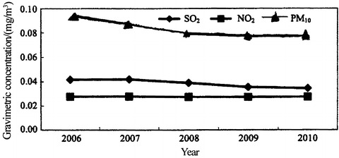
Annual variation of gravimetric concentration of SO₂, NO₂, and PM₁₀ between 2006 and 2010

Fig. 2.28.

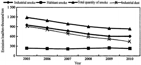
Annual variation of dust emission in the whole country and in industrial field

But it should be noted that the annual average concentration of PM_2.5 measured in China was higher than that of America by 2.8–9.7 times in 1995 [37].

It should also be mentioned that gravimetric concentration of atmospheric dust is usually used for the design of ventilation and air-conditioning system, while it is not suitable for the design of cleanroom. When it comes to the life time of air filter in air cleaning system, the gravimetric concentration is still used.

Particle Counting Concentration [38]

In the air cleaning technology field, the basis of particle counting concentration is the most commonly used particles with diameter ≥0.5 μm. Taking the stratosphere (10 km above the land) as an example, the concentration of these particles is about 20 pc/L, while the concentration above the ocean is about 2,500 pc/L. Particle counting concentration near the land differs a lot with locations and period, which is more complex than the parameter such as temperature. Therefore, in order to study the particle counting concentration of typical situations, the method to distinguish between some typical areas is adopted, which is shown in Table 2.26.

Table 2.26.

Particle counting concentration of typical areas abroad

Area	Particle concentration (≥0.5 μm)/(#/L)	Ref.	Area	Particle concentration (≥0.5 μm)/(#/L)	Ref.
County	3 × 104	[39]	Polluted area	177 × 104	[41]
Metropolis	12.5 × 104		Common area	17.7 × 104
Industrial center	25 × 104		Clean area	3.5 × 104
County	10 × 104		For design of cleanroom	17.5 × 104	[42]
Suburb	20 × 104	[40]	Specially clean	0.19 × 104
Urban	50 × 104		Specially polluted	56 × 104

In the research report “Cleanroom Calculation” from Institute of HAVC of China Academy of Building Science printed in 1977, three typical areas are used, including “industrial city,” “suburb,” and “nonindustrial area or rural area.” The corresponding atmospheric dust concentrations can be simplified as “city type,” “suburb type,” and “rural type,” which is a rough classification method. The particle counting concentration of “city type” is usually less than 3 × 10⁵ pc/L. That of “suburb type” (the industrial suburb cannot be included) is usually less than 2 × 10⁵ pc/L. That of “nonindustrial area or rural area” is usually less than 1 × 10⁵ pc/L. However, the atmospheric dust concentration of above three types only represents the average level of these areas. Taking the “city type” as an example, the concentration near the corner of area with factories surpasses the above value, and the air is close to the level of air pollution. However, with good weather or after the rainy days, the measured concentration of “city type” may be 10⁴ pc/L. But in winter, the concentration may be as large as (5–6) × 10⁶ pc/L, or even larger. When outdoor cleaning is performed and weed and leaf piled are burning, the concentration nearby can be as large as 6 × 10⁶ pc/L. The above classification was used as the calculation basis of outdoor concentration for medium-efficiency air cleaning system in “Air Cleaning Technology Measures” by 14 units in 1979.

Three years after 2005, Cui Lei et al. surveyed the atmospheric dust concentration in the whole country [43], and the data from 132 districts were summarized, which is shown in Table 2.27.

Table 2.27.

Analysis of measured data

Classification	Results
With area	Northeast 10, north China 40, east China 23, northwest 12, southwest 15, central south 32
With measuring location	Suburb 90, downtown 27, far from city 10, no locations 5
With season	Spring 20, summer 42, autumn 48, winter 22
With time	Morning 12, noon 22, afternoon 44, evening 4, no time 50
With weather condition	Sunshine 84, cloudy 8, sunny days with strong wind 4, overcast 20, Overcast with fog 2, rainy 11, rainy days with strong wind 3

Measurement results have shown that there is only one exception that the particle counting concentration for particles ≥0.5 μm is larger than 3 × 10⁵ pc/L, which was thought to be accidental.

Ten areas with the minimum and maximum concentrations are presented in Tables 2.28 and 2.29.

Table 2.28.

The minimum concentrations at ten locations

No.	Particle counting concentration (#/L)						Location	Place	Weather	Tem. (°C)	Relative humidity (%)	Wind force level
	Particle size (μm)
	0.3	0.5	0.7	1	2	5
88	2,215	1,193	583	254	85	15	Hohhot (Inner Mongolia)	Far from city	Overcast, rainy, strong winda			4–5
54	3,567	1,683	384	151	57	6	Yizhuang (Beijing)	Suburb	Sunny	31.1	18.30	2–3
125	10,085	4,976	1,958	996	368	151	Lhasa (Xizang)	Suburb	Cloudy
11	16,599	5,094	1,145	163	28	6	Dali (Yunnan)	Suburb	Sunny	26.4	53.80
37	10,014	5,309	2,326	979	248	15	Urumqi (Xinjiang)	Suburb	Sunny	29.8	18.10	2–3
113	9,964	5,608	907	281	104	16	Haikou (Hainan)	Far from city	Overcast
120	22,190	6,234	965	240	16	3	Chengmai (Hainan)	Suburb
110	12,934	6,688	2,456	517	98	18	Yinchuan ecological preservation area(Ningxia)	Far from city	Cloudy			1–2
124	20,137	8,461	2,238	446	28	6	Chuxiong (Yunnan)	Suburb	Rainy
95	19,736	9,578	2,110	340	64	7	Baoshan (Yunnan)	Downtown	Sunny

^aRefer to the analysis in the Sect. 2.6.1

Table 2.29.

The maximum concentrations at ten locations

No.	Particle counting concentration (#/L)						Location	Place	Weather	Tem. (°C)	Relative humidity (%)	Wind force level
	Particle size (μm)
	0.3	0.5	0.7	1	2	5
10	184,152	148,917	39,881	3,847	251	10	Shijiazhuang (Beijing)	Suburb	Sunny
76	182,439	156,967	57,823	8,704	868	37	Shunyi (Beijing)	Suburb	Cloudy
100	213,561	160,973	60,298	5,636	253	16	Jiaozuo (Henan)	Downtown	Overcast, rainy
40	230,630	164,485	87,424	11,171	516	33	Chengdu (Sichuan)	Suburb	Sunny	7.9	52.60	1–2
103	221,265	175,637	88,439	43,395	3,500	467	Chongwen district (Beijing)	Downtown	Overcast
70	238,886	185,804	52,518	7,888	2,044	201	Baoding (Hebei)	Suburb	Sunny
25	244,145	190,874	54,767	7,865	1,371	126	Pujiang (Chengdu)	Suburb	Overcast	10.9	55.90	1–2
67	245,500	195,517	79,065	7,654	863	95	Rongchang (Chongqing)	Suburb	Sunny	25.2	71.50
29	258,795	206,473	81,480	8,078	823	81	Qingxu (Taiyuan)	Suburb	Sunny
97	1,280,998	702,923	203,561	41,220	8,561	1,453	Cangzhou (Hebei)	Downtown	Sunny

The particle counting concentration mentioned above is not corresponding to the whole size range. When the whole particle size (mainly particle size below 0.5 μm) is used for calculation, the average concentration in the mixed layer 2 km above the land is 10⁵–10⁶ pc/L, and that near the land surface is as high as 10⁶–10⁸ pc/L, where the concentration of particles with heavy metal is about 10⁴–10⁵ pc/L [44]. In the whole size range, particles with diameter less than 0.1 μm are called condensation nucleus.

Table 2.30 shows the particle counting concentration related to air pollution event in literatures. It is shown that the concentration above 10⁶ pc/L only occurs accidentally when smog or photochemical smog is generated. The particle concentration in industrial air recommended by the USA is almost equivalent with the common industrial area in China. Therefore, 3 times of this concentration is used as the particle concentration in seriously polluted air for the outdoor calculation concentration of cleanroom, which was adopted in the monograph “Air Cleaning Technology Measures” (the reason is shown in 10.1007/978-3-642-39374-7_13).

Table 2.30.

Particle concentration in polluted air (≥0.5 μm)

Type of polluted air	Concentration (#/L)	Ref.
US industrial air	3.5 × 105	[45]
Pollution	5.6 × 105	[42]
With photochemical smog	106	[46]
Seriously polluted	1.75 × 106	[41]
Pollution	106	[47]
With smog	2 × 106	[47]
Common industrial air in China	(2–3) × 105	Measured in China

Note: Concentration of microorganism in atmospheric dust is between 1 pc/L and thousands pc/L.

Comparison Between Particle Counting Concentration and Gravimetric Concentration

There is no clear relationship between the particle counting concentration and the gravimetric concentration, because too much influence factors exist. For example, density of atmospheric dust changes with location and season. Mass increases by 10³ times when particle size increases by 10 times, so the influence of dispersity is very large. In China, the specific comparison of this aspect has not been carried out. Figure 2.29 shows the comparison of measurement at abroad [48], which can be used for reference. It is obvious that the correlation between particle counting concentration and gravimetric concentration is only valid within a range, so two dashed lines are plotted on this figure by author (in the original figure they do not exit).

Fig. 2.29.

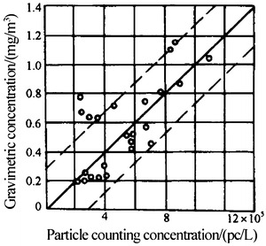
Comparison between particle counting concentration and gravimetric concentration

According to some analysis on data, the relationship among particle counting concentration, gravimetric concentration, and deposition concentration is shown in Table 2.31. In the table, several applications with extreme low particle counting concentration are also listed for comparison.

Table 2.31.

Comparison of several kinds of concentrations

Concentration	Industrial city (polluted area)	Suburb of industrial city (intermediate area)	Nonindustrial or rural area (clean area)	Cleanroom for large-scale integrated circuit	For manufacturing passive laser night vision instrument
Particle counting concentration (pc/L)	≤3 × 105	≤2 × 105	≤105	≤3	≤0.3
Weighting concentration (mg/m3)	0.3–1	0.1–0.3	<0.1
Deposition concentration [t/(km2 · month)]	>15	<15	<5

The comparison data are just for reference purpose only. In practice, when it comes to the relationship between concentrations, specific situation must be considered, and the comparison curve between particle counting concentration and gravimetric concentration under specific conditions (such as locations and seasons,) should be obtained.

Particle Size Distribution of Atmospheric Dust

Full Particle Size Distribution

With the limit of measurement means, it is really difficult to obtain the real particle size distribution of atmospheric dust accurately. Figure 2.30 shows the published data in the early of 1960s [1], which corresponds to the situation of coal smoke. The mass distribution is unimodal, but it maybe not accurate in the range of large diameter. Particle size distribution in the range of small diameter is bimodal. Since the measurement means is not known, we do not know its accuracy. From Fig. 2.31 [49], the abrupt increase of particle number for extreme small particles may occur.

Fig. 2.30.

Full particle size distribution of atmospheric dust

Fig. 2.31.

Distribution curve of airborne particles under three kinds of conditions: A small particle number in atmosphere, B near the land, C the floating of the maximum value with the increase of pollution, D near the ocean, E the background value (very clean, and the visibility is good)

Look at Fig. 2.32 published in the late of 1960s [50]; it is more close to the reality with the advancement of the measurement means. However, we know that:

1. Since the data of particle number distribution in the range of small size is lacking, the detailed information may lose. This is why it is different from the two figures above.

2. When the mass distribution is bimodal, the distribution of atmospheric dust belongs to the photochemical smog. The first peak of mass distribution including small particle size corresponds to the mass medium diameter 0.3 μm and σ _g = 2.05. The second peak of mass distribution including small particle size corresponds to the mass medium diameter 8 μm and σ _g = 2.3. There is a trough between 1 and 3 μm for this kind of distribution. The mass of particles with diameter less than 2 μm occupied 1/3–1/2 of the total mass.

Fig. 2.32.

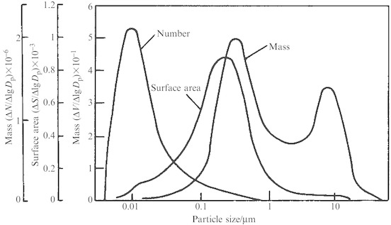
Example of full particle size distribution of atmospheric dust

In total, when the full particle size distribution of atmospheric dust is considered, the number of so-called large particles with diameter ≥0.3 μm is a very small proportion of that of condensation nucleus. The ratio varies from 1:15 to 1:5,000, or even larger [51].

From the practical application of air cleaning technology, particles with diameter larger than 0.3 or 0.5 μm are thought to be 100 %. At this time, the mass of most submicron particles only occupies 2–3 %, which is shown in Table 2.32 [52]. Moreover, submicron particles can almost penetrate air filters with performance lower than that of HEPA filters. So large difference exists when particle number and particle mass are used to evaluate the efficiency. This will be further illustrated in 10.1007/978-3-642-39374-7_4 about the characteristic of air filters.

Table 2.32.

Distribution of number and mass of atmospheric dust

Particle size interval (μm)	Average size (μm)	Number (%)		Mass (%)
		Percentage	More than 0.5 μm are considered as 100	Percentage	More than 0.5 μm are considered as 100
0–0.5	0.25	91.68	–	1	–
0.5–1	0.75	6.78	81.49	2	2.02
1–3	2	1.07	12.86	6	6.06
3–5	4	0.25	3	11	11.11
5–10	7.4	0.17	2	52	52.53
10–30	20	0.05	0.65	28	28.28

Distribution on Log-Log Probability Paper

Attenuation Distribution with Particle Size

As for the statistical distribution of atmospheric dust, particle number decreases significantly with the increase of particle size, as pointed out by Junge from Germany for the first time [53]. The relationship expression can be simplified as

2.1

where

• D _p is the particle size;

• ν is 4 for clean atmosphere, and 2.5 for smog situation;

• K is the coefficient;

• dN is the particle number of unit volume in the particle size interval from the size smaller than D _p to D _p.

This kind of distribution is shown in Figs. 2.31, 2.33 [54], and 2.34 [55]. The ordinate is the number of airborne particles within 1 cm³ air with the change of logarithmic particle radius.

Fig. 2.33.

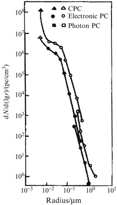
Example of measured data about airborne particle distribution in urban atmosphere

Fig. 2.34.

Measured distribution of atmospheric dust near the land: 1 average of 12 samples in the daylight (Aug.1, 1980), 2 average of 12 samples in the evening (from 19:00 of Aug.1, 1980, to 5:00 of Aug. 2, 2980), 3 fitted result with three parameters for the average of evening

From Figs. 2.32, 2.33, and 2.34, K is obtained to be 2. From Fig. 2.31, the average value of K for B, D, and E situations is about 2.

Cumulative Distribution with Particle Size on Log-Log Paper

The so-called distribution on log-log paper means the cumulative distribution of particle number with particle size on log-log paper. Before 1980s, author plotted the particle size distribution on log-log paper according to the measured data at home and abroad, which is shown in Fig. 2.35 [38]. The trend is shown obvious. In the figure, the inclination of some curve for particle size between 2 and 5 μm becomes small, which means the proportion of large particles increases. The reason may be related to the sampling. When the sampling height is not high enough, it will be greatly affected by the ground. When particle resuspension from the ground does not occur, the concentration with particles larger than 5 μm will not increase obviously during the sampling process.

Fig. 2.35.

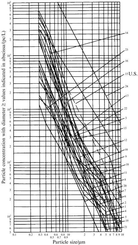
Particle size distribution of atmospheric dust before 1980s. 1 Shahe, Beijing, 2 Lintong, 3 northern suburb, Beijing, 4 Changping, Beijing, 5 Wuxi, 6 Hanzhong, 7 Beijing, 8 Beijing, 9 Beijing, 10 northern suburb, Beijing, 11 Shanghai, 12 Shanghai, 13 Huxian, 14 Tianjin, 15 industrial air of the USA, 16 Shanghai, 17 Tianjin, 18 Ōta special wards of Tokyo, Japan, 19 Hyōgo-ken outskirt, Japan, 20 Nagoya outskirt, Japan, 21 center of Kanagawa, Japan, 22 average polluted area of Tokyo, Japan, 23 clan area of Chiba-ken, Japan, 24 smog period of Tokyo, Japan

This distribution characteristic is also proved by the experiment later. Figure 2.36 is one example [56].

Fig. 2.36.

Measured distribution of atmospheric dust in Harbin

From these curves, the following relationship can be obtained [38]:

2.1

where

• is the total number of particles with diameter ≥d ₁ (pc/L);

• is the total number of particles with diameter ≥d ₂ (pc/L);

• n is the exponent of the distribution.

When the proportion of particles with diameter ≥d ₂ is considered 100 %, means the percentage of particle numbers with diameter ≥d ₁ among all particles (≥d ₂). The meaning is the same as oversize distribution in the monograph about dust removal. But the usual oversize distribution is based on gravimetric concentration, where the total quantity of particles does not have any limit of particle size. In air cleaning technology, total number of particles is based on the particles with diameter ≥0.3 or ≥0.5 μm, which depends on the measurement condition and the need. Therefore, Eq. (2.1) can also be written as

2.2

where R _d is the percentage of particles with diameter ≥d in the total number of particles with diameter ≥d ₀. That is the oversize distribution with the basis of d ₀ (%);

d is the particle size;

d ₀ is the particle size when the percentage of total particles for diameter ≥d ₀ is 100 %. Usually it is 0.3 μm or 0.5 μm.

The exponent n varies between 2 and 2.3, or sometimes it is larger than 2.3 or 3.

The data of particle size distribution for 132 areas are shown in Fig. 2.37 [43]. The particle size distributions of atmospheric dust for three kinds of areas are illustrated in Figs. 2.38, 2.39 and 2.40. The average distributions of atmospheric dust in 132 areas are shown in Fig. 2.41 [57].

Fig. 2.37.

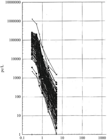
Concentration distribution of atmospheric dust in 132 areas since 2005 in China

Fig. 2.38.

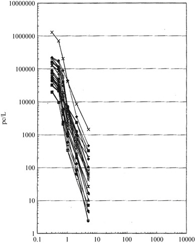
Concentration distribution of atmospheric dust in industrial cities since 2005 in China

Fig. 2.39.

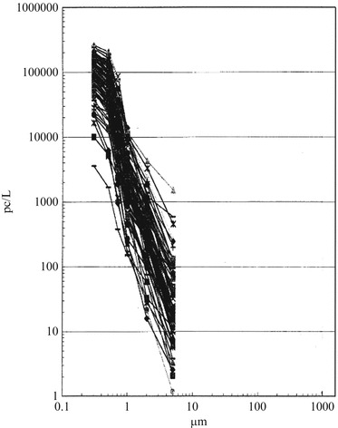
Concentration distribution of atmospheric dust in suburb areas since 2005 in China

Fig. 2.40.

Concentration distribution of atmospheric dust in nonindustrial or rural areas since 2005 in China

Fig. 2.41.

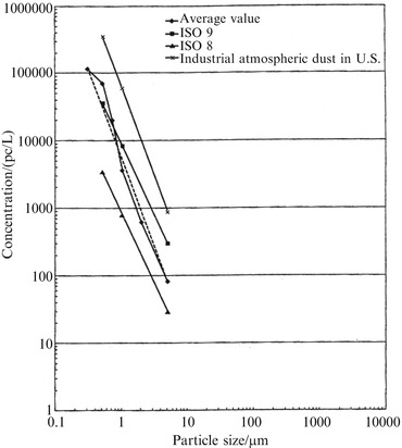
Average concentration distribution of atmospheric dust in 132 areas since 2005 in China

According to these latest measurement data, the following conclusions can be obtained:

1. The characteristic of particle size distribution of atmospheric dust is similar as that of 30 years ago.

It is known that the value of n obtained from the average distribution curve in Fig. 2.28 remains the same as that of Fig. 2.32.

• 2.The linear property of particle size distribution of atmospheric dust remains the same on log-log paper.

This kind of linear property is the total distribution characteristic, not the polygonal line from one measurement.

According to the average distribution curve in Fig. 2.38, three conclusions can be reached:

1. The inclination of the straight line between 0.5 and 1 μm becomes large, which means the proportion of particles with diameter less than 1 μm increases. This can be used to reflect the fact that with the development of economy these years, the proportion of so-called fine particles increases.

2. The inclination of the straight line between 0.3 and 0.5 μm becomes small. This may caused by the fact that the particle counter used in the experiment was calibrated with 0.5 μm standard particles, and the particle counting efficiency to measure 0.3 μm is very low. Even it reaches the counting efficiency of 0.5 μm, the inclination in this region will not decrease. So in practice, the straight line of 0.5 μm can be extended downstream, which becomes the linear relationship.

3. The particle counting concentration of atmospheric dust decreases by 30–40 % compared with the past concentration.

From Tables 2.37, 2.38 and 2.39, the current average concentrations for three kinds of atmospheric dust can be considered as less than 2 × 10⁵ pc/L, 1 × 10⁵ pc/L, and 0.7 × 10⁵ pc/L, respectively. While in the past they were 3 × 10⁵ pc/L, 2 × 10⁵ pc/L, and 1 × 10⁵ pc/L, respectively.

Table 2.37.

Influence of wind on concentration

Air velocity (m/s)	0	2	4
Concentration (pc/L)	346,000	230,000	84,000

Table 2.38.

Comparison of atmospheric dust concentrations between open space and afforest area

Distance and direction from the pollution source	Greening states	The atmospheric dust concentration (mg/m3)	Dust removal rate by greening (%)
Southeast 360 m (located at leeward direction during measurement)	Open space	1.5	53.3
	Under the sycamore forest (canopy density 0.9)	0.7
Southwest 360 m (located at leeward direction during measurement)	Open space	2.7	37.1
	Behind of the Kalopanax tree	1.4
East 250 m (located at leeward direction during measurement)	Open space	0.5	60
	Behind the sycamore forest (canopy density <0.9 with height 15 m and width 20 m)	0.2

Table 2.39.

Dust capture rate on certain types of tree leaves with unit area

Tree	Dust capture rate	Tree	Dust capture rate	Tree	Dust capture rate
Elm trees	12.27	Paper mulberry	5.87	Cherry tree	2.75
Hackberry	9.37	Trident maple	5.52	Wintersweet	2.42
Horizontal tree	8.13	Mulberry	5.39	Canada white cypress	2.06
Magnolia grandiflora	7.10	Oleander	5.28	Western catalpa	2.05
Bischofia polycarpa	6.81	Euonymus maackii	4.77	Osmanthus	2.02
Privet wood	6.63	Crape myrtle	4.42	Pittosporum	1.81
Big leaf cortex phellodendri	6.63	Sycamore	3.73	Gardenia tree	1.47
Robinia	6.37	Pomegranate	3.66	Hydrangea tree	0.63
Camphor tree	5.89	Maple	3.45
Ailanthus tree	5.88	Chinese sapium	3.39

According to Eqs. (2.1) and (2.2), the statistical distribution of atmospheric dust can be obtained, such as Tables 2.33 and 2.34. The calculation results in Table 2.34 is very close to the measured results in Table 2.32. Therefore, when total number of particles with diameter ≥d ₀ is measured, which can be used as the basis, the total number of particles with diameter ≥d can be predicted.

Table 2.33.

Statistical distribution of atmospheric dust with diameter (≥0.3 μm)

Particle size (μm)	Relative frequency (%)	Particle size (μm)	Cumulative frequency (%)	Particle size (μm)	Relative frequency (%)	Particle size (μm)	Cumulative frequency (%)
0.3	46	≥0.3	100	1.2	2	≥1.2	5
0.4	20	≥0.4	54	1.5	1	≥1.5	3
0.5	11	≥0.5	34	1.8	1	≥1.8	2
0.6	11	≥0.6	23	2.4	0.7	≥2.4	1
0.8	5	≥0.8	12	4.8	0.3	≥4.8	0.3
1.0	2	≥1.0	7

Table 2.34.

Statistical distribution of atmospheric dust with diameter (≥0.5 μm)

Particle size (μm)	Relative frequency (%)	Particle size (μm)	Cumulative frequency (%)	Particle size (μm)	Relative frequency (%)	Particle size (μm)	Cumulative frequency (%)
0.5	33	≥0.5	100	1.5	3	≥1.5	9
0.6	31	≥0.6	67	1.8	3	≥1.8	6
0.8	15	≥0.8	36	2.4	2	≥2.4	3
1.0	6	≥1.0	21	4.8	1	≥4.8	1
1.2	6	≥1.2	15

For example, when the concentration of atmospheric dust with diameter ≥0.3 μm measured by the particle counter is 3.5 × 10⁵ pc/L, what is the concentration for diameter ≥6 μm?

With Eq. (2.1), we know

It is shown that Eq. (2.1) obtained by domestic measurement can reflect the statistical distribution relationship, which is completely consistent with the result from abroad [58]. Therefore, the straight line on log-log paper can be parallel with the statistical curve of industrial atmospheric dust in USA, which means the distribution characteristics of atmospheric dust on the earth are fundamentally consistent.

In Fig. 2.42, distributions of atmospheric dust for the above four kinds of typical areas are plotted. Both the land concentration and the background concentration in Fig. 2.27 are plotted in this figure after conversion with Table 2.35. When Eq. (2.1) is used to describe these two statuses, the exponent index is approximately −2.7.

Fig. 2.42.

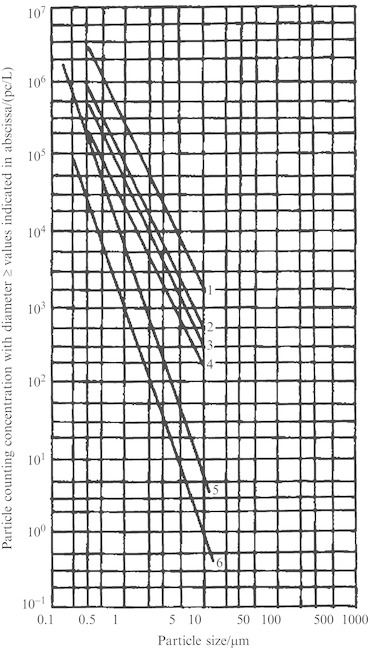
Distribution of atmospheric dust in land condition and background on log-log paper. 1 seriously polluted, 2 industrial city, 3 industrial suburb, 4 nonindustrial or rural, 5 land condition, 6 background

Table 2.35.

Calculation result with conversion

State		Concentration variation per unit particle size interval dN/dlgD p (pc/L)	Concentration variation in the particle size interval dN (pc/L)	Concentration with ≥0.1 μm (pc/L)	Concentration with ≥1 μm (pc/L)	Concentration with ≥10 μm (pc/L)	Concentration with ≥100 μm (pc/L)
B	Increase from 0.01 μm to 0.1 μm	2 × 106		2.007006 × 106
	Increase from 0.1 to 1 μm	7 × 103			0.007006 × 106
	Increase from 1 to 10 μm	7 × 100				0.000007 × 106
	Increase from 10 to 100 μm	5 × 10-4					Ignored
E	Increase from 0.01 to 0.1 μm	105		1.01001 × 105
	Increase from 0.1 to 1 μm	103			0.01001 × 105
	Increase from 1 to 10 μm	1				0.00001 × 105
	Increase from 10 to 100 μm	10-4					Ignored

Two important points can be found from Fig. 2.42. One is that the distribution of atmospheric dust is linear on log-log paper, which is a general characteristic. Of course this feature is not fit for all the specific situations. The other one is when the concentration of atmospheric dust is very low, such as the clean environment with very low background concentration, this linear characteristic is not suitable for describing particles with diameter less than 0.1 μm. This should be noted for making parallel lines corresponding to the air cleanliness level.

Why does the particle size distribution of atmospheric dust have this kind of characteristic? Someone attempted to investigate the reason in terms of the formation of some components in atmospheric dust. For example, fine particles of brittle material (such as coal and rock) generated by crush are very consistent in shape and diameter. No matter it is the crush process by mechanical means or ordinary abrasion, all the processes will generate particles with some characteristic of the diameters. This also applied to the particle size distribution of industrial particles, which is shown in Fig. 2.43 [59]. They are almost parallel. Pollen generated naturally has the distribution characteristic like Fig. 2.44 [60].

Fig. 2.43.

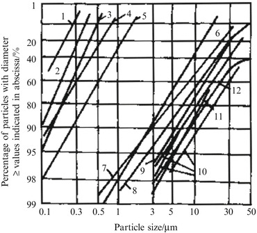
Particle size distribution of some industrial dust. 1 producer gas, 2 converter oxygen steelmaking, 3 open hearth steelmaking, 4 oxygen blowing refining lead, 5 titanium oxide, 6 tin oxide, 7 oil-fired boiler, 8 sintering furnace, 9 cement drying furnace, 10 coal-powder boiler, 11 cement aggregate drying furnace, 12 cupola

Fig. 2.44.

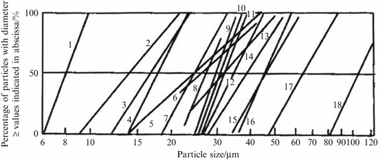
Particle size distribution of pollen spore. 1 Mimosa pudica, 2 primrose, 3 green onion, 4 balsamine, 5 purple Commelina communis, 6 pollen typhae, 7 Kalimeris indica, 8 Lycopodium, 9 dandelion, 10 phoenix-tail fern, 11 toon, 12 daisy, 13 passion flower, 14 Acacia grass, 15 tulip, 16 cuckoo, 17 rose moss, 18 hibiscus

Distribution of atmospheric dust is a very important issue. Although there are some regular patterns, it is fickle when it comes to specific distribution of atmospheric dust, which may be far away from the statistical distribution curve. It is related to many factors, which need to be discriminated and investigated specifically.

Distribution Along Vertical Height

Figures 2.42 and 2.43 show the distribution near the ground layer. The distribution at the height 50–300 m above the ground is shown in Fig. 2.45 [55]. The distribution of small particles with radius r _p < 3 μm is basically linear, which is similar as that near the ground.

Fig. 2.45.

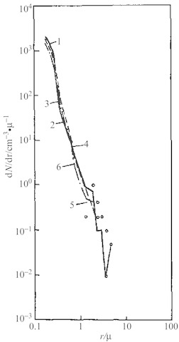
Measured distribution of atmospheric dust with height (20:00–21:06, Aug.1, 1980): 1 50 m, 2 100 m, 3 150 m, 4 200 m, 5 250 m, 6 300 m

According to the solid line representing the relationship between measured concentration and height in Fig. 2.46, the relationship can also be expressed with the dashed line, which is obtained with the least square fit method for the measured data. Therefore, the relationship between the average concentration of atmospheric dust at height Z (N _Z) and the concentration on ground (N ₀) is [55]

2.3

where a parameter H _p is introduced, which is called the reference height for atmospheric aerosol, H _p = 1.41 km, which is equivalent with the reference height under muddy atmospheric condition (the visibility distance in the evening and cloudy days is 5 km).

Fig. 2.46.

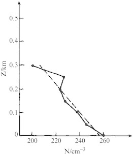
Agreement between fitted vertical distribution and measured distribution

It is obvious that it is not applicable for describing the atmospheric dust concentration below 50 m with Eq. (2.3). The first reason is that data are lacking in Fig. 2.46 within the height 50 m above the ground. The second reason is that the situation close to the ground is very complex. Figure 2.47 shows one example of atmospheric dust concentration on the vertical direction within 50 m from the ground [51]. It is clear that the concentration becomes the maximum when near the ground and decreases sharply as it becomes higher. The second maximum appears about 22 m above on the ground which is on the roof (it is the chimney that takes particles to the atmosphere). The third one is about 50–60 m high, which is the exhaust pollution layer by factory. If the traffic volume is small, the first layer with the maximum concentration appears 20 m above the ground [61], which is shown in Table 2.36.

Fig. 2.47.

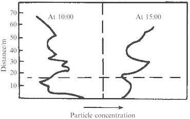
Vertical distribution of atmospheric dust in the center of Leipzig

Table 2.36.

One example for the vertical distribution of atmospheric dust

Height from floor (m)	Atmospheric dust concentration (pc/L)
	≥0.5 μm	≥0.5 μm
1	3.19 × 104	49
17	4.33 × 104	29
30	3.98 × 104	28

In short, due to the different environmental conditions, there may be maximum values of first layer, second layer, or even third layer in the vertical distribution of dust concentration. Usually, the dust concentration within the height 5–15 m above the ground is less affected by the ground and so it is more stable. Therefore, the Japan Environmental Agency set the atmospheric dust sampling height to be 5–10 m in the relevant regulations. In China, the “Global Atmospheric Monitoring Work Regulations” laid out by the Environmental Sanitation Monitoring Station under Chinese Academy of Medical Sciences also set the dust sampling height above 3–4 m.

Influencing Factors for Concentration and Distribution of Atmospheric Dust

Influence of Wind

In modern cities, atmospheric dust is mainly produced from point source (chimney and other emission device), line source (streets that are crowded with cars), and area source (industrial district). The most important means of propagating pollutions are through the wind.

The common impression that people have about wind is that wind always comes with dusts together. But this only shows the case that wind blows up the dusts on the ground. For example, in spring and winter in Beijing, the wind that contains the dusts from the Mongolian Plateau can make the sky dark yellow. In most cases in general, the pollutant concentration in the atmosphere is directly proportional to the total emission amount and inversely proportional to the average wind speed. So if the wind speed increases two times, the leeward pollutant concentration will be reduced by half. This is the common sense in the field of environmental protection. One relevant professional research report abroad mentions that, when the precise particle counter was used carefully to study the properties of atmospheric dust, it can be found that wind is the factor that causes the low atmospheric dust concentration measurable [48, 62]. For example, when the wind changes from 0 to 4 m/s, the variation of dust concentration can be seen on Table 2.37 [51].

Figure 2.48 is the measured results on a typhoon day [63], and the synchronism between concentration and the wind speed is quite obvious. A small delay can also be seen. The minimum value of the concentration appears just after the maximum speed. It is quite easy to understand the inversely proportional relationship between concentration and wind speed, as shown in Fig. 2.49. Of course, the sand storm is the exception.

Fig. 2.48.

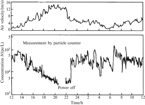
Relationship between wind speed and concentration (Sept. 17, 1965)

Fig. 2.49.

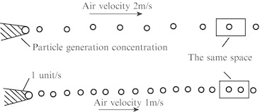
Schematic of the effect of wind

As China is located in the eastern coast of Eurasia with the mid or low latitude, the west wind is blocked by the Qinghai-Tibet Plateau and is disturbed by the monsoon. As a result, the northwest wind prevails in winter for most eastern areas from north of the Great Wall to the Hainan Island. The southwest monsoon prevails in the southwest part of China in winter. In spring, the wind changes from northerly winds to southerly winds. And in autumn, the monsoon direction is just opposite as that in spring.

As a result, in the eastern monsoon region, there are two prevailing wind directions. For example:

• Shenyang: southerly wind 26 %; northerly wind 17 %

• Beijing: northerly wind 26 %; southerly wind 15 %

• Jinan: southwest wind 20 %; northeast wind 17 %

• Wuhan: northerly wind 21 %; northeast wind 17 %; southeast wind 15 %

• Nanjing: northeast wind 21 %; southeast wind 19 %

• Guangzhou: northerly wind 17 %; east wind 16 %; southeast wind 14 %

Since there are two prevailing wind directions, in reality the concept is meaningless that pollution can be avoided at the weather side of the prevailing wind direction. The influence of the wind not only depends on the wind frequency, but also depends on the wind speed. When both the frequency and the wind speed are low, the pollution on the lee side may become larger. Therefore, the concept of pollution wind frequency is proposed [64], i.e.,

or

For example, at Fengtai of Beijing, the north wind prevails in winter with wind frequency 17 %. In summer, the frequencies of southwest wind and south wind are 17 % and 14 %, respectively. The wind speed in summer is low. According to the calculation of pollution wind frequency, the southwest wind is the most important prevailing wind in the whole year. One thing to be mentioned here is that “prevailing wind direction” has been replaced by “dominant wind direction” at first and later by “wind frequency direction with the minimum pollution,” according to the relevant national regulations.

The pollution wind frequency has important implications for the location of cleanroom. When there is only one main prevailing wind direction, it’s better to place the cleanroom and clean area in the weather side of the prevailing wind direction. When there are two prevailing wind directions, they should be built at one side. In Fig. 2.50, northerly wind is opposite compared with southerly wind. In this condition, cleanroom or clean area should be placed on either left down or right up of the general drawing. The middle is for the general area. The so-called pollution area includes the boiler chamber, the coal site, the building construction site, and the workshop emitting pollution. The so-called general area includes the general workshop and the working facility. Whether the clean area should be placed on left down or right up, the wind frequency on both left and right sides should also be further considered. If the wind frequency at the right side (pollution wind frequency) is the minimum, cleanroom should be placed on the left down corner, and the pollution area should be on the right up side.

Fig. 2.50.

Example I of determining the location for cleanroom with the pollution wind frequency

In Fig. 2.51, the two prevailing wind directions are intersecting, so the cleanroom or clean area should be placed on the right.

Fig. 2.51.

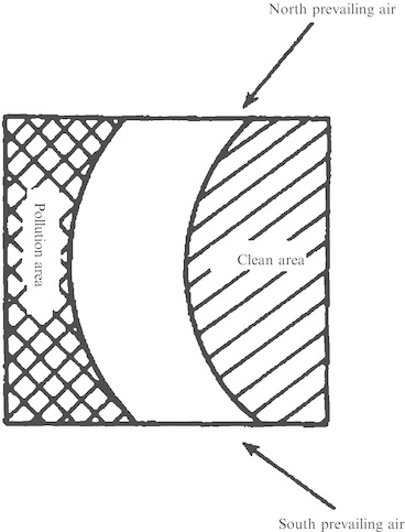
Example II of determining the location for cleanroom with the pollution wind frequency

About the pollution wind frequency, readers can refer to author’s book “Application of Air Cleaning Technology” (China Building Industry Press, 1989).

Influence of Humidity [65]

Basic Process

At the beginning of this chapter, it has pointed out that generally the atmospheric dust contains both solid particles and liquid particles. Particles with diameter between 0.001 and 0.1 μm belong to the range of permanent atmospheric dust, but they are called specially as condensation nucleus.

Condensation nucleus can be divided into two parts. One is easy to absorb water and can be easily dissolved by water, such as NaCl and sulfate, which belongs to soluble condensation nuclei. Another one is not dissolved by water but can be wetted by water like soil particle, ore particle, and soot particle, which are called hygroscopic condensation nuclei.

The generation amount of soluble condensation nuclei such as sulfate is mainly dependent on the amount of sulfuric acid mist formed by the reaction of moisture and SO₂. Therefore, the content of moisture in air, i.e., the absolute humidity, is the important factor for the generation amount of this kind of particles. Soluble condensation nuclei start to become solution after absorbing moisture, which enlarges itself gradually.

For non-soluble condensation nuclei, the process of water vapor condensation depends on the degree of supersaturation (E _rm is the saturation vapor pressure of droplet; E is the saturation vapor pressure of air). When the condensation nuclei are large, the degree of supersaturation on surface needed for condensation is smaller, which means the allowable E is larger and the relative humidity of air can be smaller. On the contrary, with the larger relative humidity, the smaller condensation nuclei can still be wetted to large diameter.

So it is not complete if we hold the view that only relative humidity or absolute humidity is the factor influencing the atmospheric dust concentration. Absolute humidity mainly influences the moisture absorption of soluble condensation nucleus, while further dissolution and enlargement of condensation nucleus (the latter case includes insoluble condensation nucleus) mainly depend on relative humidity.

Someone once gave this idea [1] that when the relative humidity φ reaches 95 %, the radius of particle will be enlarged by 1.3 times, compared with the case φ = 40 %.

As the particle counter usually has a lower limit of the measurable radius, a large amount of unmeasurable particles will exceed the lower limit and enter to the range that can be measured when condensation nucleus becomes big as it absorbs water vapor. That makes not only the concentration of atmospheric dust count big, but also the proportion of small particles large. If light scattering optical particle counter or photoelectric turbidimeter is usually used to measure the concentration of atmospheric dust, we’ll discover that the concentration, especially that of small particles, in the morning is much bigger than others. That is caused by the high humidity in the morning (of course the noise of water vapor molecules may cause overlying influence on the instrument). So do not be surprised when we meet this situation; concentration will reduce after the sunrise. But the concentration is still higher than that in other times.

The following is the specific measurement result.

Figure 2.52a is the measurement result from abroad [48], where the particle counter manufactured in the USA was used. In the figure, the black dot represents the measurement data with relative humidity below 80 %. It is shown with this kind of high relative humidity, most of the measurement data fall in the lower part of the chart, which means the proportion of particle number with diameter larger than 1 μm to that with diameter larger than 0.3 μm reduces. At this time, the number of small particles increases, while that of big particles reduces correspondingly. In summer from mould rainy days to the summit of summer, the humidity is high. The number of small particles measured is very large. Besides, since the humidity varies a lot, the particle size distribution is extremely unstable. This is the reason why the relative humidity limit is set in the fractional efficiency method with atmospheric dust in China, which is used to measure the efficiency of air filter (refer to 10.1007/978-3-642-39374-7_16).

Fig. 2.52.

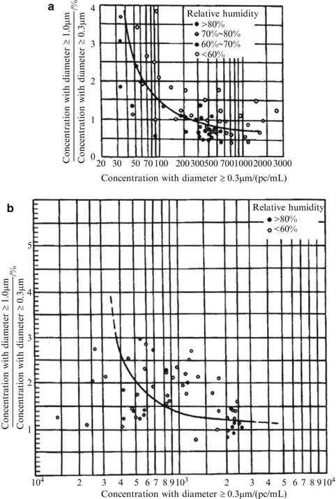
Relationship between relative humidity and the proportion of small particles

Figure 2.52b illustrates the measurement data with domestic made particle counter, which has the same trend. But due to the lack of the data with small concentrations, it is not so obvious as the above picture.

Related Extent

Figures 2.53 and 2.54 show the example of variations of meteorological parameters, including particle counting concentration with atmospheric dust, the relative humidity, and the absolute humidity in “nonindustrial area or rural area” [59]. In the diagram, the ordinate is expressed with the water vapor partial pressure e with the unit mbar. In the range of normal temperature, 1 mbar = 0.75 mm of mercury. From the chart, the variation trend of daily atmospheric dust concentration is basically the same as that of the relative humidity.

Fig. 2.53.

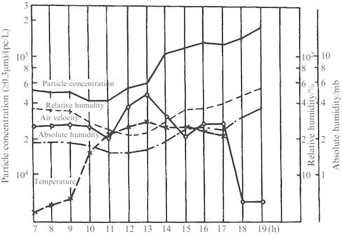
Variation of atmospheric dust in one day at Xinglong of Hebei on March 15, 1980

Fig. 2.54.

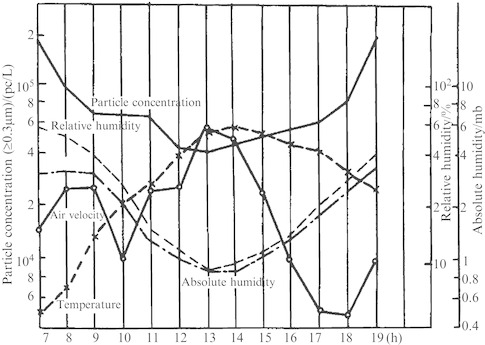
Variation of atmospheric dust in one day at Xinglong of Hebei on March 16, 1980

Both relative humidity and absolute humidity have influence on atmospheric dust concentration. But there is no solid proof to show which influence is more prominent. But according to the analysis of some measurement result, the relative humidity is thought to have more influence on the atmospheric dust concentration than the absolute humidity. This opinion is possible when the relative humidity has influence on the increase of the condensation nuclei according to the above analysis.

Daily Variation Model of Atmospheric Dust

It is really very complicated for the daily variation of atmospheric dust concentration. But the trend can be seen from Figs. 2.53, 2.54, and 2.55. The atmospheric dust concentration generally appears the crest in the morning (7–9 A.M.) and the afternoon (17–19 P.M.), while the trough appears at noon or afternoon.

Fig. 2.55.

Variation of atmospheric dust in one day at Xinglong of Hebei between March 17 and 18, 1980

Figures 2.56, 2.57, and 2.58 show the daily variation of atmospheric dust concentration for the “city type” and “suburban type.” Due to the influence factors of urban atmospheric dust concentration are more complex, this can be also seen from these figures. The daily variation of atmospheric dust in city is more complex than that of the rural area. A few small peaks and small wave trough may occur in a day period. However, the peaks in the morning and evening and the troughs around noon are obvious. Figure 2.59 is one example of atmospheric dust concentration measured abroad [58]. The arrow is added by author during quote, where this trend is also shown. Relevant literatures with the trend are also presented, which will not be quoted here one by one.

Fig. 2.56.

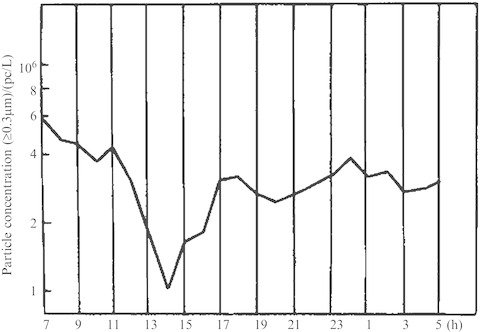
Daily variation of atmospheric dust concentration under the iron tower at Deshengmen of Beijing between August 1 and 2, 1980

Fig. 2.57.

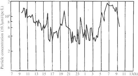
Daily variation of atmospheric dust concentration in Shanghai on Dec. 24, 1975

Fig. 2.58.

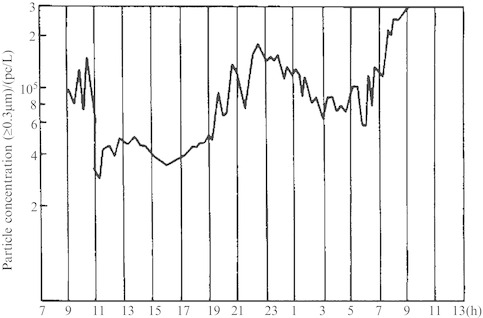
Daily variation of atmospheric dust concentration in northwest region on April 20, 1976

Fig. 2.59.

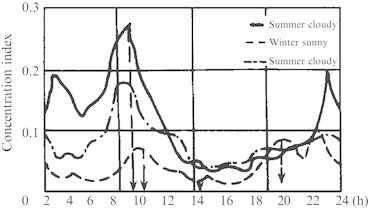
Example of daily variation of atmospheric dust concentration in Japan

Therefore, author puts forward a model that can be used to illustrate this trend. It is the W-type model conceived as in Fig. 2.60. The upper part of the figure is mainly influenced by the daily variation of humidity, while the lower part is also affected by other factors. The former is the “rural type,” and the latter is the “city type.” The reason to cause the daily variation of atmospheric dust concentration may be related to the influence factors for the trend of daily variation of the humidity and SO₂. Several measurements have proved that the daily variation of these two parameters also has W type [66, 67].

Fig. 2.60.

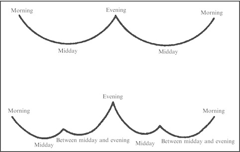
W-type model of atmospheric dust concentration

The above model further needs some measurement proof, and Fig. 2.61 [56] is an example.

Fig. 2.61.

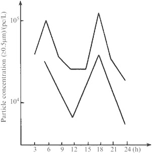
Daily variation of atmospheric dust concentration in Harbin

Influence of Afforestation

The afforest has a certain effect of reducing the atmospheric dust concentration. Table 2.38 is the comparison of atmospheric dust concentration in open space and afforest area [68].

According to research, when the tree has the following characteristics, the width of leaf is large, the leaf stretches flat and rigidly, the leaf is not easily swayed, the leaf surface is rough and full of fur, and the number of leaves is large, then this kind of tree is conducive to remove dust. For example, the sycamore has a high collection efficiency of dust, which has tall canopy, dense leaves, and large total leaf surface. Table 2.39 has listed the data of dust collection quantity by certain kinds of tree leaves.

Distribution of Atmospheric Microorganism

Concentration Distribution

To study the atmospheric microorganism, distributions of bacterium and fungus are mainly investigated, which should be measured by the classification sampler such as Anderson sampler. The classification characteristic of standard Anderson sampler is shown in 10.1007/978-3-642-39374-7_16.

There is some research showing that distributions of both bacterium and fungus have certain patterns. Figure 2.62 shows the concentration variation of atmospheric bacteria in the Xidan commercial district in Beijing. Figure 2.63 shows the concentration variation with fractional size. Figures 2.64 and 2.65 show the data in Fengtai, Beijing [69]. From these measurements, the following conclusions can be obtained:

1. There are two peaks and two wave troughs for the concentration of atmospheric bacteria and fungi within a day.

2. Two peaks appear at about 7:00 A.M. and 22:00 P.M. In the morning, one reason is that both the activity of people and vehicle on the road increases; the other reason is that the atmosphere near the ground is under the steady state with temperature inversion, and the velocity is small that causes the flow rate of atmosphere small, as well as the small radiation intensity. Both of these two reasons result in the first peak. At nightfall, the activity of people and vehicle on the road increases, while the radiation disappears; this has no effect of killing the generated microorganism. So the second peak is formed.

3. Two troughs appear at about 13:00 P.M. and 1:00 A.M. At noon, the air temperature increases gradually and the wind velocity increases. The steady state of atmosphere is destroyed. The atmospheric dust containing microorganism at the lower layer of atmosphere is taken away to the sky by the dispersion of vertical flow stream, and then diluted [69]. Another reason is that the sterilization effect by solar radiation increases. So the first trough is formed at 13:00 P.M. In the midnight, although there is no solar radiation, the generation amount of bacteria decreases sharply since all the activity on the ground reduces and it is close to be static. This is good for the deposition of big particles. So the second trough is formed.

4. The concentration of atmospheric bacteria is positively correlated with that of atmospheric dust.

5. Concentration is large for the season with the large sandy wind. For example, concentrations between March and May, as well as between September and November, are higher than that of other months in Beijing (Fig. 2.66).

Fig. 2.62.

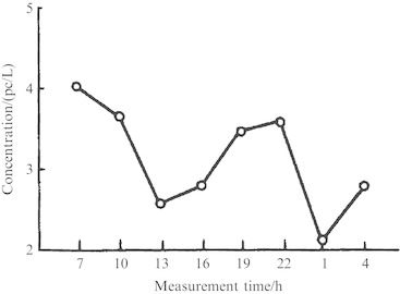
Daily variation of atmospheric bacteria concentration in Xidan

Fig. 2.63.

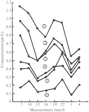
Daily variation of atmospheric bacteria concentration with fractional size in Xidan. 1 the first class, 2 the second class, 3 the third class, 4 the fourth class, 5 the fifth class, 6 the sixth class

Fig. 2.64.

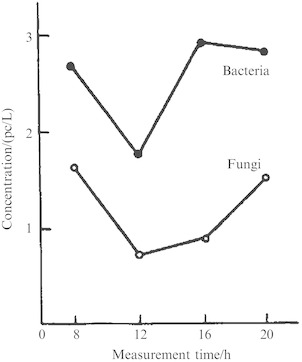
Daily variation of atmospheric bacteria and fungi concentration in Fengtai.

Fig. 2.65.

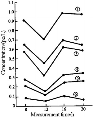
Daily variation of atmospheric bacteria concentration with fractional size in Fengtai (the meanings for the labels from 1 to 6 are the same as that of Fig. 2.62)

Fig. 2.66.

Daily variation of atmospheric fungi concentration with fractional size in Fengtai (The meanings for the labels from 1 to 6 are the same as that of Fig. 2.63)

Particle Size Distribution

Figure 2.67 shows the particle size distribution data of atmospheric bacteria and fungi in Xidan district of Beijing [70]. It is shown that the medium diameter of atmospheric bacteria in Xidan approaches the maximum value 8.1 μm at 13:00 P.M. and the minimum value 6.1 μm at 1:00 A.M. That of atmospheric fungi approaches the maximum value 4.5 μm at 13:00 P.M. and the minimum value 3.6 μm at 22:00 P.M. The variation patterns are opposite as that of concentration. It is obvious that the larger the particle size is, the more the deposition is, which will cause the concentration smaller. It should be noted that the particle diameter is not the naked diameter of bacteria, but the carrier diameter (refer to the equivalent diameter introduced in 10.1007/978-3-642-39374-7_9). The particles with larger diameter are likely to be killed by the ultraviolet ray exposure of solar radiation [71].

Fig. 2.67.

Daily variation of atmospheric bacteria and fungi concentration in Xidan

From four season’s point of view, the variation of particle diameter for atmospheric bacteria and fungi is small, as shown in Fig. 2.68 [70].

Fig. 2.68.

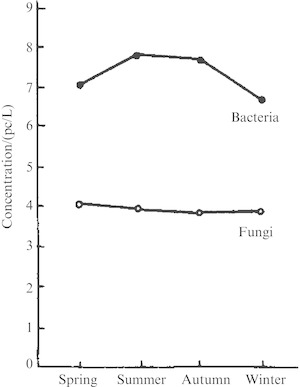
Seasonal variation of atmospheric bacteria and fungi concentration in Xidan

The similar trend is also reflected in the measurement results from other places [72].

References

- 1.Fett V. Atmospheric dust. Moscow: Publishing House of Foreign Literature; 1961. [Google Scholar]
- 2.Fuchs HA (1960) The mechanics of aerosols (trans: Gu Zhenchao). Science Press, Beijing (In Chinese)
- 3.Tsziri A Measurement method of weight and humidity for aerosol. J Jpn Air Clean Assoc. 1973;12(4):20–53. [Google Scholar]
- 4.Harada A (1973) Background pollution of atmosphere, Technical reports of the Meteorological Research Institute, Japan (In Japanese)
- 5.Beijing Evening News (1998) p 15, 4 Apr 1998 (In Chinese)
- 6.Jin H, Ouyang N, Cheng ZF . Environmental management and technology. Beijing: China Environmental Science Press; 1994. [Google Scholar]
- 7.Jin H, Ouyang N, Cheng ZF . Environmental management and technology. Beijing: China Environmental Science Press; 1994. [Google Scholar]
- 8.UNEP Urban air pollution (continued) World Environ. 1993;2:29–34. [Google Scholar]
- 9.Peng JX (2000) Review and inspiration of global environment and its development during the past century. In: China environment yearbook 2000. China Environmental Science Press, p 580 (In Chinese)
- 10.Editorial Board of “China Environment Yearbook” (2001) China environment yearbook. China Environmental Science Press, Beijing, p 524 (In Chinese)
- 11.Katsunori H Research on the generation of particles by photochemical reaction. J Jpn Air Clean Assoc. 1975;12(5):16–25. [Google Scholar]
- 12.Katsunori H. Measurement and monitoring of pollution structure and air cleanliness level indoors. Mag Build Equip. 1967;202:39. [Google Scholar]
- 13.Ishibashi T, Nishiwaki J (1966) Department of Public hazard. Hygiene Engineering III (In Japanese)
- 14.Wang MX, Lv WX, Ren LX, Winchester JW. Sampling and chemical analysis technology of atmospheric aerosol. Tech Equip Environ Pollut Control. 1981;2:1–10. [Google Scholar]
- 15.Huang SQ, Kong FC, Jian JS, Xu GP, Luo JH, He RY. Measurement of microelement in airborne particles by emission spectra. Tech Equip Environ Pollut Control. 1981;2:24–131. [Google Scholar]
- 16.Zhou BB, Xu JL, Hu GY. Characteristics of metal elements in the atmospheric Particulate of Shanghai. Shanghai Environ Sci. 1994;13(9):30. [Google Scholar]
- 17.Ruzyllo J, Hattori T, Opila RL, Novak RE (1978) Cleaning technology in semiconductor device manufacturing. The Electrochemical Society, Inc., Translated by No. 10 Design Institute of the former Fourth Ministry of Machinery and Industry (In Chinese)
- 18.Control of environment, supply and material in the manufacturing process of integrated circuit (1973) Kejicankao Newspaper (semiconductor) 2 (In Chinese)
- 19.Zhu T, Bai ZP, Chen W Source analysis of air particulate in Qinhuangdao city. Res Environ Sci. 1995;8(5):49–55. [Google Scholar]
- 20.Lv JM, Takeshi Y Performance of salt particles by air filter. J Jpn Air Clean Assoc. 1993;31(1):12–19. [Google Scholar]
- 21.Institute of Scientific and Technical Information of China (1973) Atmospheric pollution and control (No. 10 Survey of foreign hazardous matters) (In Chinese)
- 22.Saito Y Epidemiology of pollen. J Jpn Air Clean Assoc. 1972;9(8):7–14. [Google Scholar]
- 23.Zai I State of the environment in high-rise buildings observed with the management method. J Jpn Air Clean Assoc. 1975;74:27–44. [Google Scholar]
- 24.Katsunori H Recent development of the measurement method for indoor air pollution. J Jpn Air Clean Assoc. 1975;74:13–26. [Google Scholar]
- 25.Motomura K Study on indoor air pollution. J Jpn Air Clean Assoc. 1976;14(4):23–31. [Google Scholar]
- 26.Ishizuki J et al (1988) Statistical study of the atmospheric aerosol concentration as the design load for air cleaning device. Part I: In Tokyo area. Proceedings of the 7th air cleaning and pollution control conference. Japan Air Cleaning Association (In Japanese)
- 27.Wang SL, Chai FH, Yang TX Characteristics analysis of elements contained in air suspended particles with different sizes in Beijing. Res Environ Sci. 2002;15(4):10–12. [Google Scholar]
- 28.Jiang HM, Wang DY Research development of inhalable particulate in atmosphere. Environ Sci Trend. 2001;1:11–14. [Google Scholar]
- 29.Zhang WL, Xu DQ, Cui JS The characteristics and toxic mechanism of fine particle pollution (PM2.5) in air. Environ Monit China. 2002;18(1):59–62. [Google Scholar]
- 30.Yang FMY, Ma YL, He KB. Research profile of fine atmospheric particulate matter PM2.5. World Environ. 1991;4:32–340. [Google Scholar]
- 31.Zhou CY, Ye RQ, Tang GC Study of organic pollutants in aerosol and its distribution pattern. China Environ Sci. 1991;11(5):337–340. [Google Scholar]
- 32.Editorial Board of “China Environment Yearbook” (2001) China environment yearbook. China Environmental Science Press, p 598 (In Chinese)
- 33.1993 China environment yearbook. China Environmental Science Press (1993), p 522 (In Chinese)
- 34.2005 China environment yearbook. China Environmental Science Press (2005), p 774 (In Chinese)
- 35.Ministry of Environmental Protection of the People’s Republic of China (2011) 2006–2010 environmental report of China. China Environmental Science Press, Beijing, pp 10 –35 (In Chinese)
- 36.Ministry of Environmental Protection of the People’s Republic of China report on the state environment in China. Environ Protect. 2002;6:6. [Google Scholar]
- 37.Wei FW, Teng EJ, Wu GP, Wu GP, Wilson WE, Chapman RS. Concentration and elemental components of PM2.5, PM10 in ambient air in four large Chinese cities. Environ Monit China. 2001;17(7):1–6. [Google Scholar]
- 38.Xu ZL (1980) Particle counting concentration and particle size distribution of atmospheric dust in China 1(4): 20–23 (In Chinese)
- 39.Нонезов РТ, Знаменский РЕ. Обеспыливание воздушной среди в “Чесмых комнатах”. Водоснабжение и Санитарная Техника. 1973;3:29–32. [Google Scholar]
- 40.Fujisaki H Actual performance of cleaning device in precision processing factory. Jpn Air Cond Heat Refrig News. 1971;11(10):99–108. [Google Scholar]
- 41.Hirasawa K Planning and design of cleanroom. Jpn Air Cond Heat Refrig News. 1973;13(1):75–88. [Google Scholar]
- 42.Kanai K Design and operation of cleanroom. J Jpn Air Clean Assoc. 1971;8(2):63–83. [Google Scholar]
- 43.Cui L, Xu ZL, Wang R, et al. Particle number concentration of atmospheric particles in China. J HV&AC. 2008;38(7):1–5. [Google Scholar]
- 44.Motomura K Measurement method of relative humidity for aerosol. J Jpn Air Clean Assoc. 1974;12(4):61–69. [Google Scholar]
- 45.Austin PR, Timmerman SW. Design and operation of clean rooms. Detroit: Business News Publications; 1965. [Google Scholar]
- 46.Hirasawa K Impact of atmospheric pollution on industrial products and medicine and its countermeasures. Jpn Air Cond Heat Refrig News. 1970;10(2):33–40. [Google Scholar]
- 47.Noda K Cleanroom for precision processing factory. Jpn Air Cond Heat Refrig News. 1970;10(10):64–75. [Google Scholar]
- 48.Niitsu Y et al (1967) Study on property of atmospheric aerosol (the 2nd report). J SHASE Jpn 41(4):1–8 (In Japanese)
- 49.Reeves RG, Anson A, Landen D (1979) Manual of remote sensing, vol I: Theory, instruments and techniques (trans: Tang Dingyuan, Chen Ningqiang). National Defence Industry Press, Beijing (In Chinese)
- 50.Hinds WC (1989) Aerosol technology: properties, behavior, and measurement of airborne particles (trans: Sun Yufeng, Chapter 14). Heilongjiang Science and Technology Press, Harbin (In Chinese)
- 51.Kratzer PA (1963) Climate of city (trans: Xie Kekuan). China Industrial Press, Beijing (In Chinese)
- 52.Fukuyama H. Airborne matter- nature and role. J SHASE Jpn. 1975;49(8):57–60. [Google Scholar]
- 53.Junge CE (1953) Die Rolle der Aerosole und der Gasformigen Beimengungen der Luft im Sprenstoffhaushalt der Troposphare, Tellus 1953, 5(1) (cited from Aerosol Handbook, translated by Zhou Jinqin, 1981) (In Chinese)
- 54.Whitby KT, Liu BYH (1969) Atmospheric aerosol size distributions. Preprint of P,T.S., pp 36–46
- 55.You RG, Hong ZX, Lv WX, et al. Spatial distribution variation of atmospheric aerosol concentration and scale in boundary layer. Chin J Atmos Sci. 1983;7(1):88–94. [Google Scholar]
- 56.Wei XM Analysis of the variation of atmospheric dust. Contam Control Air Condit Technol. 1987;3:7–8. [Google Scholar]
- 57.Cui L, Xu ZL, Wang R, et al. Characteristic of atmospheric particles in China. J HV&AC. 2008;38(5):10–12. [Google Scholar]
- 58.Dorman RG. Dust control and air cleaning. Oxford: Pergamon Press; 1974. [Google Scholar]
- 59.Oono C Duct collation technology, pollution control measures and technological development. Extra Edition of PPM. 1972;7:106–142. [Google Scholar]
- 60.Miyu S, et al. Measurement of particle size distribution and density for pollen and spores. J Soc Powder Technol. 1972;9(2):102–104. [Google Scholar]
- 61.Uchiyama M. Investigation result on the design and construction of cleanroom. J SHASE Jpn. 1972;46(4):19–25. [Google Scholar]
- 62.Senuma I Variation of airborne particle in outdoor air and its influence on indoor environment. Proc Jpn Build Inst. 1960;64:79–85. [Google Scholar]
- 63.Niitsu Y, Yoshikawa S, Tomita H (1966) Study on property of atmospheric aerosol (the 1st report). J SHASE Jpn 40(11):1–13 (In Japanese)
- 64.Urban geography group at Department of Geology and Geography (1974) Beijing University, Wind and Urban Planning. Environmental Protection 2:16–23 (In Chinese)
- 65.Xu ZL, Wu ZW Influence of humidity on particle counting concentration of atmospheric particles. China Environ Sci. 1982;6:59–65. [Google Scholar]
- 66.Liu WJ, Zhao GZ Meteorological field structure and atmospheric concentration in Shenyang. Environ Sci. 1981;2(2):26–31. [Google Scholar]
- 67.Wang SF Mode for air pollution evaluation in suburb of Beijing. China Environ Sci. 1981;1:46–53. [Google Scholar]
- 68.Institute of Botany at Jiangsu Province Effect of air purification with urban greening. Environ Sci. 1978;6:49–51. [Google Scholar]
- 69.Hu QX, et al. Atmospheric microorganism concentration in Beijing and Tianjin areas. Environ Sci. 1989;10(5):31–35. [Google Scholar]
- 70.Hu QX, et al. Particle size of atmospheric microorganism in Beijing. China Environ Sci. 1992;12(4):296–299. [Google Scholar]
- 71.Che FX Effect of solar radiation on killing the airborne microbe. Disinfect Steriliz. 1985;2(2):101–105. [Google Scholar]
- 72.Hu QX et al (1994) Study of atmospheric microorganism–median diameter and particle size distribution of atmospheric bacteria 10(6):37–38 (In Chinese)