Importance of Stability Analysis When Using Nonlinear Semimechanistic Models to Describe Drug‐Induced Hematotoxicity

Abstract

Stability analysis, often overlooked in pharmacometrics, is essential to explore dynamical systems. The model developed by Friberg et al.¹ to describe drug‐induced hematotoxicity is widely used to support decisions across drug development, and parameter values are often identified from observed blood counts. We use stability analysis to study the parametric dependence of stable and unstable solutions of several Friberg‐type models and highlight the risks associated with system instability in the context of nonlinear mixed effects modeling. We emphasize the consequences of unstable solutions on prediction performance by demonstrating nonbiological system behaviors in a real case study of drug‐induced thrombocytopenia. Ultimately, we provide simple criteria for identifying parameters associated with stable solutions of Friberg‐type models. For instance, in the original Friberg model, we find that stability depends only on the parameter that governs the feedback from peripheral cells to progenitors and provide the exact range of values that results in stable solutions.

Study Highlights.

• WHAT IS THE CURRENT KNOWLEDGE ON THE TOPIC?

☑ Stability analysis is an established tool for the analysis of complex mathematical models, which is widely used in fields such as mathematical and systems biology, but it is often overlooked in pharmacometrics, where system behaviors are mainly explored with computational methods (e.g., simulations).

• WHAT QUESTION DID THIS STUDY ADDRESS?

☑ This study identifies the parameter region associated with the stability of the classical Friberg model ¹ and four additional drug‐induced hematotoxicity models.

• WHAT DOES THIS STUDY ADD TO OUR KNOWLEDGE?

☑ We demonstrate that the feedback parameter γ controls the stability of the homeostatic equilibrium in the Friberg model, ¹ and it can cause instability issues above a critical value (γ* = 0.5685…). This results in unreliable model predictions, as we highlight in the analysis of a real case study of drug‐induced thrombocytopenia.

• HOW MIGHT THIS CHANGE DRUG DISCOVERY, DEVELOPMENT, AND/OR THERAPEUTICS?

☑ Prediction performance can be highly affected by model instability, which does not guarantee a correct application of a model when describing hematopoiesis during homeostasis and subjected to perturbations. Therefore, we highly recommend incorporating the results of this analysis when modeling drug‐induce hematotoxicity.

Stability analysis, the theory that characterizes the stability of the equilibria of a dynamical system, ² , ³ is a key principle in fields such as mathematical biology and engineering and systems control, where analytical methods are regularly used to study the properties of dynamical systems. ⁴ , ⁵ In pharmacometrics, however, although differential equations are routinely used to describe pharmacokinetics and pharmacodynamics relationships, ⁶ , ⁷ stability analysis is often overlooked, and rather exploratory computational methods (e.g., sensitivity analysis, simulations), which are not exhaustive, ⁸ represent the main approach to investigate model behaviors. ⁹ In the pharmacometrics field, parameter values are thereby optimized by fitting models to physiological and rich data sets, which are in some cases sufficient to avoid the appearance of unstable solutions. However, the high quality of these data sets does not guarantee the identification of stable solutions in models that are often highly empirical, with only some mechanistic elements. In fact, nonlinear models can exhibit various and counterintuitive behaviors, which are difficult to reveal through simulations alone. ⁹ In this context, applying standard techniques for stability analysis provides a deep understanding of the system dynamics, such as the spectrum of behaviors within the parameter space. ⁹ Ultimately, this is essential to provide reliable predictions. ⁹

In stability analysis, a critical point defines the conditions for a dynamical system to be in equilibrium, which can be stable or unstable. ³ From a mathematical point of view, blood homeostasis can be seen as a stable equilibrium point. We remark that for homeostasis to prevail, the model parameter values must ensure the stability of this equilibrium. ² , ³ In this regard, in a recent publication, ¹⁰ MacLean et al. ¹¹ showed that a niche‐mediated signaling feedback governs hematopoietic stem cell niche dynamics and regulates stability. The disruption of these controling mechanisms leads to system instability and dysfunction of the hematopoiesis process, which may result in disease development. Moreover, stability analysis techniques can be applied to reveal novel insights into the hematopoietic process. ¹² In this respect, Weston et al. ¹³ used stability analysis to explore the concentration‐dependent behavior of granulocyte‐colony and macrophage‐colony stimulating factor‐induced differentiations, and showed that the granulocyte‐colony stimulating factor may encourage monopoiesis under some conditions, whereas the macrophage‐colony stimulating factor always inhibits granulopoiesis.

The model by Friberg et al. ¹ is widely used to describe drug‐induced hematotoxicity. For the full comprehension of the application of this model to describe hematopoiesis during homeostasis and subjected to perturbations, we performed a formal stability analysis. We have identified one critical point and characterized how the stability of the hematopoietic cell populations depends on the model parameter values. In this way, we can reliably predict the long‐term effects of drug‐induced perturbations. For instance, if this equilibrium point is stable, blood cell counts return to homeostatic values after drug‐induced perturbations, whereas perturbations grow bigger and bring the counts away from baseline values if unstable.

Here, we use these techniques from dynamical system analysis to gain new insights into the relationship between the parameters of the Friberg model and its temporal behavior. We derive the stability region of the system and we emphasize the risks associated with model instability through the analysis of a real case study of drug‐induced thrombocytopenia. In addition, we present four variations of the classical Friberg model, ¹ where we change some of the assumptions on model parameter values. We derive the stability regions of these four additional drug‐induced hematotoxicity Friberg‐type models, and we discuss these results in the context of nonlinear mixed effects modeling, highlighting the consequences in prediction performance, and providing recommendations for future analyses.

METHODS

Model description

Friberg et al. ¹ characterized the effects of oncology drugs on hematopoiesis using the following set of differential equations, which comprise the proliferation of progenitors in the bone marrow, cell maturation through a set of transit compartments, release of mature cells into circulation, and a regulatory feedback loop from peripheral blood cells to proliferative progenitors (Figure  1 ):

$$\begin{array}{c}\frac{\text{dProl}}{\mathrm{d}t}=k_{\text{prol}}\text{Prol}{\left(\frac{{\text{Circ}}^{\ast }}{\text{Circ}}\right)}^{\gamma }\left(1-\text{Edrug}\right)-k_{\mathit{tr}}\text{Prol},\\ \frac{{\text{dTransit}}_1}{\mathrm{d}t}=k_{\text{tr}}\text{Prol}-k_{\text{tr}}{\text{Transit}}_1,\\ \frac{{\text{dTransit}}_2}{\mathrm{d}t}=k_{\text{tr}}{\text{Transit}}_1-k_{\text{tr}}{\text{Transit}}_2,\\ \frac{{\text{dTransit}}_3}{\mathrm{d}t}=k_{\text{tr}}{\text{Transit}}_2-k_{\text{tr}}{\text{Transit}}_3\\ \frac{\text{dCirc}}{\mathrm{d}t}=k_{\text{tr}}{\text{Transit}}_3-k_{\text{circ}}\text{Circ}.\\ \end{array}$$ (1)

Prol, Transit₁, Transit₂, Transit₃, and Circ are state variables representing bone marrow proliferating cells, three transit cell compartments, and circulating cells, respectively. k _prol, k _tr, and k _circ are the rates of cell proliferation, maturation, and clearance from blood, and they are defined in terms of the mean transient time (MTT):

$$k_{\text{prol}}=k_{\text{tr}}=k_{\text{circ}}=\frac{4}{\text{MTT}}.$$ (2)

Figure 1.

Schematic representation of the semimechanistic model of drug‐induced bone marrow toxicity developed by Friberg et al. ¹ The rat and the human symbols that are superimposed to the variable representing the circulating cells in the blood show that the model can be applied to both clinical and preclinical data sets where drug‐induced myelosuppression is quantified by peripheral cell counts. Circ, circulating cells in the blood; fdbk, feedback; k _circ, rate of clearance from blood; k _prol, proliferation rate; k _tr, maturation rate; Prol, proliferative cells; Prolif, proliferative; T₁, Transit_1 cells; T₂, Transit_2 cells; T₃, Transit_3 cells.

Circ* is the size of the compartments in homeostatic equilibrium, or baseline values, which are also assumed to be equal, and they are quantified by the number of observed circulating cells in the blood in homeostasis, as follows:

$$X^{\ast }=\left({\text{Prol}}^{\ast },{\text{Transit}}_1^{\ast },{\text{Transit}}_2^{\ast },{\text{Transit}}_3^{\ast },{\text{Circ}}^{\ast }\right)=\left({\text{Circ}}^{\ast },{\text{Circ}}^{\ast },{\text{Circ}}^{\ast },{\text{Circ}}^{\ast },{\text{Circ}}^{\ast }\right)$$ (3)

Edrug is a function of the drug concentration in the plasma over time that characterizes the drug effects on proliferative bone marrow progenitors, and from a mathematical point of view, this corresponds to introducing perturbations into the system. Perturbations activate the feedback loop mechanism described in Eq. 1 by the following term:

$${\text{feedback}}_{\text{Circ}}={\left(\frac{{\text{Circ}}^{\ast }}{\text{Circ}}\right)}^{\mathrm{\gamma }}$$ (4)

which increases/decreases the proliferation of progenitors accordingly to the difference between the number of circulating cells and their baseline value to repristinate the homeostatic equilibrium (X*).

The initial values to solve Eq. 1 are assumed to be equal to the baseline values for each cell population when we assumed that the hematopoietic system is initially in equilibrium, exhibiting homeostatic cell counts:

$$\text{Prol}(0)=T1(0)=T2(0)=T3(0)=\text{Circ}(0)={\text{Circ}}^{\ast }$$ (5)

Linear stability analysis

Stability, or bifurcation, analysis is usually carried out by linearizing the system of differential equations (Eq. 1) around the critical point of interest (X*) and characterizing the long‐term system behavior in the neighborhood of the critical point (X*). ² , ³ , ⁴ Practically, this corresponds to investigating the system eigenvalues (λs), which are the roots of the characteristic equations associated with the linearized system. ² , ³ , ⁴

In the absence of drug, the Friberg model (Eq. 1) has only one point of equilibrium (X*), defined in Eq. 3, which corresponds to baseline values for all cell populations, i.e., X* is the homeostatic equilibrium. Depending on the dose schedule and duration of treatments, almost stable drug concentrations in tissues over time may emerge and lead to the appearance of other equilibrium points. However, we focused our analysis on the common scenario of the loss and recovery of homeostasis as a drug is added and cleared from the body, which implies that only one equilibrium point emerges in the absence of drug. Therefore, we analyzed the model in Eq. 1 in the absence of drugs (i.e., Edrug = 0) and simulated the effects of drug‐induced perturbations by initializing model simulations from values of cell counts different from the homeostatic equilibrium X* (Eq. 3).

The characteristic equation corresponding to the Friberg model (Eq. 1) is

$$P\left(\lambda \right)=\left|J-\lambda I\right|={\lambda }^5+4{\lambda }^4{k}_{\mathit{tr}}+6{\lambda }^3{k}_{\mathit{tr}}^2+4{\lambda }^2{k}_{\mathit{tr}}^3+\lambda k_{\mathit{tr}}^4+\gamma k_{\mathit{tr}}^5=0$$ (6)

where I is the identity matrix, and J is the Jacobian matrix, about the equilibrium point X ^*, associated with Eq.  1:

$$J=\left[\begin{array}{ccccc}0& 0& 0& 0& -\gamma k_{\mathit{tr}}\\ k_{\mathit{tr}}& -k_{\mathit{tr}}& 0& 0& 0\\ 0& k_{\mathit{tr}}& -k_{\mathit{tr}}& 0& 0\\ 0& 0& k_{\mathit{tr}}& -k_{\mathit{tr}}& 0\\ 0& 0& 0& k_{\mathit{tr}}& -k_{\mathit{tr}}\end{array}\right]$$ (7)

From bifurcation theory, ² , ³ we know that the stability of an equilibrium X* is characterized by the sign of the real parts of the solutions of Eq.  5 (i.e., the system eigenvalues λs). In particular, X* is stable if all these real parts (Re(λ)) are negative, unstable if Re(λ) > 0, and further analyses are required to assess stability when eigenvalues λs are pure imaginary numbers.

To investigate the signs of Re(λ) we solved the Routh‐Hurwitz conditions ⁴ using Mathematica (version 11.0; Wolfram Research, Inc., Champaign, IL). Bifurcation analysis was performed using the bifurcation software Oscill8 Dynamical Systems Toolset ¹⁴ (Supplementary Material s).

Modifications of the Friberg model

The classical Friberg model can be expanded and/or updated to include additional features based on the type of data measurements and the prior knowledge available. ¹⁵ Four examples of variations of the Friberg model are detailed in the following sections, and these new systems (Table  1 ) are presented using their associated Jacobian matrixes about the homeostatic equilibrium point X ^*.

Table 1.

Comparison between the classical Friberg model ¹ and some of its variations

Model	Feature	Data	Stability region
Friberg	Model parameters: Three Circ0, γ, MTT Transit compartments: Three	Blood cell counts	$\gamma \le 0.568542$
A	Model parameters: Three Circ0, γ, MTT Transit compartments: Variable	Blood cell counts	$\gamma \le f\left(n\right)\sim \frac{1.9}{n}$
B	Model parameters: Four Circ0, Prol0, γ, MTT Transit compartments: Three	BM progenitor and blood cell count	$\gamma \le f\left(\frac{Pr{\text{ol}}^{\ast }}{{\text{Circ}}^{\ast }}\right)$
C	model parameters: Three Circ0, γ, MTT Transit compartments: Three	Blood cell counts	$\gamma \le f(\text{MTT})$
D	Model parameters: Four Circ0, Prol0, γ, MTT Transit compartments: Three	BM progenitor and blood cell counts	$\gamma \le f\left(\frac{{\text{Prol}}^{\ast }}{{\text{Circ}}^{\ast }},\text{MTT}\right)$

Model A: Variable number of transit compartments. Model B: The number of proliferative progenitor cells is estimated from data. Model C: Proliferation rate is independent of maturation time. Model D: Hypotheses from models B and C together. More details on these models and their stability regions are reported in Figure  3 .

BM, bone marrow; Circ, circulating cells in the blood; MTT, mean transit time; Prol, proliferative cells.

Model A: Variable number of transit compartments

The number of transit compartments is set equal to three in most applications of the Friberg model, ¹⁵ , ¹⁶ but the length of this maturation chain can be modified if prior knowledge is available or to improve the characterization of the data. ¹⁶ , ¹⁷

Assuming that the number of transit compartments is equal to n ≥ 1, the Jacobian (about the homeostatic equilibrium) associated with the system becomes:

$$J=\left[\begin{array}{ccccc}0& 0& 0& \cdots & -\gamma k_{\mathit{tr}}\\ k_{\mathit{tr}}& -k_{\mathit{tr}}& 0& \cdots & 0\\ 0& k_{\mathit{tr}}& -k_{\mathit{tr}}& \cdots & 0\\ ⋮& ⋮& ⋮& \ddots & ⋮\\ 0& 0& 0& \cdots & -k_{\mathit{tr}}\end{array}\right].$$ (8)

Model B: The number of proliferative progenitor cells is estimated from data

When the number of proliferating progenitor cells in the bone marrow is available, ¹⁸ Prol* is estimated directly from the data, and the homeostasis conditions expressed in Eqs. 2 and 3 become:

$$k_{\text{prol}}=k_{\text{tr}}=k_{\text{circ}}\frac{{\text{Circ}}^{\ast }}{{\text{Prol}}^{\ast }}$$ (9)

and

$$X^{\ast }=\left({\text{Prol}}^{\ast }{\text{,Transit}}_1^{\ast }{\text{,Transit}}_2^{\ast }{\text{,Transit}}_3^{\ast }{\text{,Circ}}^{\ast }\right)=\left({\text{Prol}}^{\ast }{\text{,Prol}}^{\ast }{\text{,Prol}}^{\ast }{\text{,Prol}}^{\ast }{\text{,Circ}}^{\ast }\right)$$ (10)

respectively.

The Jacobian (about the homeostatic equilibrium) associated with this new system is:

$$J=\left[\begin{array}{ccccc}0& 0& 0& 0& -\gamma k_{\text{circ}}\\ k_{\text{circ}}\frac{\text{Circ}\ast }{\text{Prol*}}& -k_{\text{circ}}\frac{\text{Circ}\ast }{\text{Prol}\ast }& 0& 0& 0\\ 0& k_{\text{circ}}\frac{\text{Circ}\ast }{\text{Prol}\ast }& -k_{\text{circ}}\frac{\text{Circ}\ast }{\text{Prol}\ast }& 0& 0\\ 0& 0& k_{\text{circ}}\frac{\text{Circ}\ast }{\text{Prol}\ast }& -k_{\text{circ}}\frac{\text{Circ}\ast }{\text{Prol}\ast }& 0\\ 0& 0& 0& k_{\text{circ}}\frac{\text{Circ}\ast }{\text{Prol}\ast }& -k_{\text{circ}}\end{array}\right]$$ (11)

Also, as in Eq. 2, k _circ is defined in terms of the MTT.

Model C: Proliferation rate is independent of maturation time

As previously reported, ¹⁹ the cell production rate is independent of cell maturation time; therefore a new parameter

$$a=\frac{3}{\text{MTT}}$$ (12)

can be used to describe the maturation rate within the chain of transit compartments in Eq. 1. ¹⁹ The homeostasis conditions expressed in Eqs. 2 and 3 become:

$$k_{\text{prol}}{\text{Prol}}^{\ast }=k_{\text{tr}}{\text{Prol}}^{\ast }=k_{\text{circ}}{\text{Circ}}^{\ast }$$ (13)

$${\text{Prol}}^{\ast }{=\text{Circ}}^{\ast }{\text{; Transit}}_1^{\ast }{=\text{Transit}}_2^{\ast }{=\text{Transit}}_3^{\ast }{=\text{Circ}}^{\ast }\frac{k_{\text{circ}}}{a}$$ (14)

and the elimination rate of mature cells from blood (k _circ) is fixed using the literature value of the cell half‐life. ¹⁷ , ¹⁹

The Jacobian (about the homeostatic equilibrium) associated with this new system is:

$$J=\left[\begin{array}{ccccc}0& 0& 0& 0& -\gamma k_{\mathit{tr}}\\ k_{\mathit{tr}}& -a& 0& 0& 0\\ 0& a& -a& 0& 0\\ 0& 0& a& -a& 0\\ 0& 0& 0& a& -k_{\mathit{tr}}\end{array}\right]$$ (15)

Model D: (i) The number of proliferative progenitor cells is estimated from data, and (ii) the proliferation rate is independent of maturation time

The last case study comprises a system made with three transit compartments for which the number of progenitor cells Prol* is known from data (i.e., hypothesis used in model B), and where the proliferation rate (k _prol) is independent of the maturation time (MTT) (i.e., hypothesis in model C).

The Jacobian (about the homeostatic equilibrium) associated with this new system is:

$$J=\left[\begin{array}{ccccc}0& 0& 0& 0& -\gamma k_{\text{circ}}\\ k_{\mathit{circ}}\frac{{\text{Circ}}^{\ast }}{{\text{Prol}}^{\ast }}& -a& 0& 0& 0\\ 0& a& -a& 0& 0\\ 0& 0& a& -a& 0\\ 0& 0& 0& a& -k_{\text{circ}}\end{array}\right]$$ (16)

The stability regions of these new four systems (Eqs. 7, 10, 14, and 15) were identified using the method previously described for the stability analysis of the Friberg model.

RESULTS

The stability of the Friberg model depends on the parameter (γ) that governs the strength of the feedback mechanism from peripheral cells to bone marrow progenitors

As described in the Methods section, the equilibrium of a system in a critical point (X^*) is asymptotically stable when the eigenvalues of the linearized equations have negative real parts (i.e., Re(λ) < 0). For the classical Friberg model (Eq.  1), we found that the stability of the homeostatic equilibrium X^* (Eq. 3) depends only on the parameter that describes the strength of the feedback from circulating cells to bone marrow proliferative progenitors, γ. The range of values for γ that ensures the stability of the homeostatic equilibrium (i.e., model solutions will converge to baseline values) is as follows:

$$0\le \gamma \le -56+40\sqrt{2}={\gamma }^{\ast }=0.568542\dots$$ (17)

From bifurcation analysis we know that γ* is a supercritical Hopf bifurcation point ² , ³ that represents the emergence of a family of stable periodic solutions (known as stable limit cycles) from the stable equilibrium (X^*), which loses its stability for values of γ greater than γ*. Precisely, γ* is associated to a pair of complex conjugate eigenvalues that cross the imaginary axis (i.e., Re(λ) = 0), leading to a positive real component. When the real part changes sign, the stable homeostatic equilibrium becomes unstable and trajectories start to wind away from it, growing in time until they are captured by a (small amplitude) stable limit cycle. ² , ³ In this respect, the bifurcation plot in Figure  2 a shows the region of stability of the system and how the equilibrium X^* loses its stability when γ crosses the critical point γ*, exhibiting growing oscillations (red and green lines). Simulations generated using a value of γ within the stability region, and challenged with a perturbation (i.e., starting in a neighborhood of the equilibrium), converge to the homeostatic equilibrium X^*, and they represent the physiological response of hematopoiesis to a perturbation, e.g., drug‐induced cytopenia (Figure  2 b1,c1). Conversely, when γ takes the value of the bifurcation point γ*, a periodic limit cycle solution appears (Figure  2 b2,c2) with amplitude zero at γ = γ*, and for any initial conditions Eq. 1 evolves into this oscillatory solution. As we know from the Hopf bifurcation theorem, ² , ³ whenever a stable equilibrium loses its stability through a supercritical Hopf bifurcation point, there is always born a family of stable limit cycles, whose amplitude increases when γ moves away from the Hopf bifurcation point γ* (Figure  2 b3,c3). Stable limit cycles attract model trajectories, and they have been used to describe the dynamics of periodic hematological diseases, such as cyclic neutropenia, ²⁰ , ²¹ cyclic thrombocytopenia, ²² or periodic chronic myelogenous leukemia. ²¹ , ²³ However, when γ is far away from the stability threshold γ*, the disruption of the homeostatic equilibrium (X^*) results in growing oscillations that are attracted by a limit cycle whose big oscillations do not describe a physiological response of hematopoiesis to a challenge (Figure  2 b3,c3).

Figure 2.

The stability of the homeostatic equilibrium X* (Eq. 3) of the Friberg model ¹ changes according to the values of the parameter γ that governs the feedback from the peripheral blood cells to the bone marrow progenitors values. Bifurcation diagram: on crossing the bifurcation point γ*, the homeostatic steady state (solid black line) becomes unstable (dotted black line), and a family of periodic limit cycle solutions appears (solid red and green lines show the maximum and minimum of the oscillations, respectively, in the log scale) (a). γ* is called a supercritical Hopf bifurcation point, and it is characterized by a change in stability of the steady state X* as γ crosses the bifurcation line. This bifurcation plot was generated with the Oscill8 Dynamical Systems Toolset. ¹⁴ Circulating cells over time (b). Phase plane showing circulating cells vs. proliferative cells (c). Each number (1–3) corresponds to a different value of the parameter γ, and plots can be grouped in the following three scenarios: b1–c1 γ < γ*, stable homeostatic equilibrium: Oscillations from the steady state decay quickly over time and an open trajectory converging to the equilibrium point appears in the phase plane. b2–c2 γ ~ γ*: A small amplitude limit cycle solution is born in the vicinity of the stable homeostatic equilibrium. b3–c3 γ > γ*, unstable homeostatic equilibrium: Growing oscillations wind away from the steady state, but they are attracted by stable limit cycles, resulting in periodic oscillations over time, which correspond to a close trajectory in the phase plane. The values of the model parameters used to generate trajectories are the following: baseline of 1 × 10⁹ cells/L (Circ*), mean transit time of 125 hours, no drug effect, and γ values are reported above each plot. Initial conditions for the number of circulating cells (Circ): 0.2 × 10⁹ cells/L while all the other variables were set equal to Circ* (1 × 10⁹ cells/L) at time 0. Initial conditions are illustrated by the blue point in each phase plane plot, and they correspond to small perturbations of the steady state. Circ, circulating cells in the blood.

Singular modifications of the Friberg model largely impact the stability region

The stability condition on the parameter γ that governs the feedback mechanism (Eq. 16) derives from the model structure itself and its homeostasis conditions, and it is therefore independent of the other parameter values, and of the type of hematological toxicity or perturbation under analysis.

If we alter the model structure in Eq. 1 to introduce new features (e.g., an increased/decreased number of transit compartments), new stability conditions will arise for the system, but the behaviors will be similar, with the model losing its stability and starting to exhibit growing oscillations when parameter values exit the stability region.

Model A: Increasing the number of transit compartments shrinks the stability region

Model A (Eq. 7) provides a generalization of the classical Friberg model, ¹ which comprehends a number n ≥ 1 of transit compartments. Under this setting, the stability region does not depend solely on the parameter γ that governs the feedback mechanism, as per the Friberg model (γ ≤ 0.56…), but it is determined by both γ and the number of transit compartments (n ≥ 1) (Figure  3 , model A). In other words, the stability region is defined by the following monotonically decreasing function of n ≥ 1 (with n the natural number):

$$\gamma \le {\gamma }^{\ast }=f\left(n\right)\sim \frac{1.9}{n}$$ (18)

Figure 3.

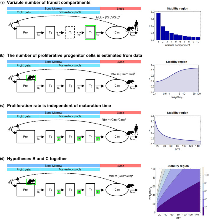
Stability regions of drug‐induced cytopenia models that were built on the original Friberg model. ¹ The first column shows model diagrams, and the stability regions are on the right. Within each diagram, modifications from the classical Friberg model ¹ are highlighted in green. Also, the data required to parameterize each model are identified by the rat or human symbol, and they are superimposed to the corresponding type of cells. Model A: Variable number of transit compartments. Model B: The number of proliferative progenitor cells is estimated from the data. Model C: Proliferation rate is independent of maturation time. Model D: Hypotheses from models B and C together. More details on these models and their stability regions are reported in Table  1 . Circ, circulating cells in the blood; fdbk, feedback; k _circ, rate of clearance from blood; k _prol, proliferation rate; k _tr, maturation rate; MTT, mean transit time; Prol, proliferative cells; Prolif, proliferative; T_i, Transit_i cells; T_N, Transit_N cells; T₁, Transit_1 cells; T₂, Transit_2 cells; T₃, Transit_3 cells.

This means that the value γ* decreases for the increasing number of transit compartments (Figure  3 , model A). Also, at least one compartment is required to have bifurcation, and if the system was reduced to only proliferative and mature cells (i.e., Prol and Circ), then the homeostatic equilibrium would be always stable.

Model B: Increasing the ratio between the number of proliferative and circulating cells enlarges the stability threshold γ*

The usage of model B (Eq. 10) may require knowledge about peripheral blood cells and bone marrow progenitor populations. ¹⁸ In this model, the parameter Prol*, which describes the homeostatic number of progenitor cells, is not assumed to take the same value as the number of mature cells (Circ*). This feature is reflected in the stability region of model B, which depends on γ and on the ratio between the size of the proliferative compartment (Prol*) and the number of circulating cells (Circ*) (Figure  3 , model B). Moreover, similarly to model A, the stability region of Eq. 10 is expressed by the following monotonically increasing function of Prol*/Circ*:

$$\begin{array}{c}\gamma \le {\gamma }^{\ast }=f\left(\frac{{\text{Prol}}^{\ast }}{{\text{Circ}}^{\ast }}\right)\\ =\frac{0.5\left(-24-45\frac{{\text{Prol}}^{\ast }}{{\text{Circ}}^{\ast }}-34{\left(\frac{{\text{Prol}}^{\ast }}{{\text{Circ}}^{\ast }}\right)}^2-9{\left(\frac{{\text{Prol}}^{\ast }}{{\text{Circ}}^{\ast }}\right)}^3\right)}{\frac{{\text{Prol}}_0}{{\text{Circ}}_0}}\\ +0\text{.5}\sqrt{\frac{576+2192\frac{{\text{Prol}}^{\ast }}{{\text{Circ}}^{\ast }}+3753{\left(\frac{{\text{Prol}}^{\ast }}{{\text{Circ}}^{\ast }}\right)}^2+3588{\left(\frac{{\text{Prol}}^{\ast }}{{\text{Circ}}^{\ast }}\right)}^3+1998{\left(\frac{{\text{Prol}}^{\ast }}{{\text{Circ}}^{\ast }}\right)}^4+612{\left(\frac{{\text{Prol}}^{\ast }}{{\text{Circ}}^{\ast }}\right)}^5+81{\left(\frac{{\text{Prol}}^{\ast }}{{\text{Circ}}^{\ast }}\right)}^6}{{\left(\frac{{\text{Prol}}^{\ast }}{{\text{Circ}}^{\ast }}\right)}^2}}\\ \end{array}$$ (19)

Therefore, increasing the ratio between the size of the proliferative compartment and mature cell number results in increasing values of the stability value γ* (Figure  3 , model B).

Model C: Increasing the maturation time shrinks the stability region

In model C (Eq. 14) the cell production rate is not assumed to depend on the cell maturation time. Under this setting, the stability region depends on the parameter γ that governs the feedback mechanism and on the maturation time (MTT) (Figure  3 , model C). The stability region is defined by the following monotonically decreasing function of MTT:

$$\begin{array}{c}\gamma \le {\gamma }^{\ast }=f\left(\text{MTT}=\frac{3}{a}\right)\\ =\frac{0.5\left(-24a^3-45a^2{k}_{\mathit{tr}}-34a{k}_{\mathit{tr}}^2-9k_{\mathit{tr}}^3\right)}{a{k}_{\mathit{tr}}^2}\\ +0.5\sqrt{\frac{576a^6+2192a^5{k}_{\mathit{tr}}+3753a^4{k}_{\mathit{tr}}^2+3588a^3{k}_{\mathit{tr}}^3+1998a^2{k}_{\mathit{tr}}^4+612a{k}_{\mathit{tr}}^5+81k_{\mathit{tr}}^6}{a^2{k}_{\mathit{tr}}^4}}\\ \end{array}$$ (20)

Similarly to what showed for model A, the value γ* decreases for increasing values of the mean transit time (Figure  3 , model C).

Model D: The stability region depends on both maturation time and size of compartments

Model D is built combining models B and C, and this is therefore reflected in its stability region, which depends on (i) the parameter γ that governs the feedback mechanism, (ii) the ratio between the size of the proliferative compartment (Prol*) and the number of circulating cells (Circ*), and (iii) on the maturation time (MTT) (Figure  3 , model D). Consequently, the stability region is defined by the following function of Prol*/Circ* and MTT:

$$\begin{array}{c}\gamma \le {\gamma }^{\ast }=f\left(\frac{{\text{Prol}}^{\ast }}{{\text{Circ}}^{\ast }},\frac{3}{a}\right)\\ =\frac{0.5\left(-24a^3\frac{{\text{Prol}}^{\ast }}{{\text{Circ}}^{\ast }}-45a^2\frac{{\text{Prol}}^{\ast }}{{\text{Circ}}^{\ast }}{k}_{\text{circ}}-34a\frac{{\text{Prol}}^{\ast }}{{\text{Circ}}^{\ast }}{k}_{\text{circ}}^2-9\frac{{\text{Prol}}^{\ast }}{{\text{Circ}}^{\ast }}{k}_{\text{circ}}^3\right)}{a{k}_{\mathit{circ}}^2}\\ +0\text{.5}\sqrt{\frac{576a^6{\left(\frac{{\text{Prol}}^{\ast }}{{\text{Circ}}^{\ast }}\right)}^2+2192a^5{\left(\frac{{\text{Prol}}^{\ast }}{{\text{Circ}}^{\ast }}\right)}^2{k}_{\text{circ}}+3753a^4{\left(\frac{{\text{Prol}}^{\ast }}{{\text{Circ}}^{\ast }}\right)}^2{k}_{\text{circ}}^2+3588a^3{\left(\frac{{\text{Prol}}^{\ast }}{{\text{Circ}}^{\ast }}\right)}^2{k}_{\text{circ}}^3+1998a^2{\left(\frac{{\text{Prol}}^{\ast }}{{\text{Circ}}^{\ast }}\right)}^2{k}_{\text{circ}}^4+612a{\left(\frac{{\text{Prol}}^{\ast }}{{\text{Circ}}^{\ast }}\right)}^2{k}_{\text{circ}}^5+81{\left(\frac{{\text{Prol}}^{\ast }}{{\text{Circ}}^{\ast }}\right)}^2{k}_{\text{circ}}^6}{a^2{k}_{\text{circ}}^4}}\\ \end{array}$$ (21)

Figure  3 , model D depicts the contour plot that represents the surface defined in Eq. 20, and it shows how the region of stability changes under the effect of increasing maturation times and compartment sizes.

Impact of stability analysis on a case study where the Friberg model was used to describe the thrombocytopenia effects induced by a bromodomain‐containing protein 4 (BRD4) inhibitor (AZD5153)

Collins et al. ²⁴ modeled the thrombocytopenia risk associated with AZD5153, a selective bromodomain‐containing protein 4 (BRD4) inhibitor, using the myelosuppression model described in Eq. 1 (classical Friberg framework). The model was first fitted to platelet counts from preclinical studies in rat and then used to make clinical predictions at anticipated therapeutic doses and schedules.

As discussed in the original publication, ²⁴ the data set generated in the preclinical studies was small, with nine rats across three dosing groups and 54 observations in total. Samples were collected from each rat prior to the start of dosing (to establish platelet baseline values) on 3 days during dosing (to evaluate the nadir) and on another 3 days postdosing (to assess recovery). Therefore, because of the reduced size of this study, some uncertainty was expected in the identification of parameter values. ²⁴ Fitting the thrombocytopenia model (Eq. 1) to the AZD5153 rat data presented in ref. 24 (Figure  4 a) resulted in a value of the parameter γ outside the stability region (γ = 0.7; Table  2 ), which therefore generated solutions characterized by sustained oscillations that do not converge to the homeostatic equilibrium (but to a stable limit cycle), consequently unreliable for extrapolation purposes (Figure  4 b,c). Note that oscillatory solutions were also obtained when using the nonlinear mixed effect approach to estimate parameter values (data not shown). The stable drug‐induced oscillations resulted in platelet counts never returning to physiological values (Figure  4 b). In essence, after the drug treatment, hematopoiesis homeostasis was no longer achievable by the model, although in reality, in the treated animals, we observed that drug‐induced myelosuppression is reversed after suspending the treatment. Furthermore, using the oscillatory solutions of the model to simulate the effects of new and untested regimens (e.g., repeated dosing cycles) resulted in predictions where drug effects exacerbate after each cycle as a consequence of the unstable nature of the homeostatic equilibrium and not because platelet progenitors had become more sensitive to the drug (Figure  4 c). Therefore, because in the absence of drug‐induced perturbations the healthy biological hematopoietic system does not exhibit sustained oscillations, any simulation run using a value of γ outside the stability region (e.g., γ = 0.7) would result in an unreliable prediction.

Figure 4.

Simulations of AZD5153‐induced thrombocytopenia with an unstable model result in unreliable predictions. Two AZD5153 dosing regimens were simulated: 1.5 mg/kg daily for 10 days (first column) and 1 mg/kg twice daily, 3 days on, 4 days off (second column). Blue points represent AZD5153 data, ²⁴ whereas black lines show model simulations converging to the homeostatic equilibrium (continuous line, γ = 0.4) and to the limit cycle (dotted line, γ = 0.72), respectively. Predictions are shown for the same doses and time points as in the observed data (a). Predictions are shown for the same doses tested in the preclinical studies but over a longer time period than the one sampled in the data (b). Simulations generated with γ = 0.72 do not converge to the homeostatic equilibrium, i.e., system homeostasis is lost. Predictions are shown of repeated cycles of treatments that represent new and untested regimens (c). Simulations generated with γ = 0.72 predicted exacerbated toxicity, but this is only a consequence of the oscillatory nature of the trajectories, which are attracted by a stable limit cycle and therefore do not converge to the homeostatic equilibrium. Parameter values used in the simulations are reported in Table  2 . All simulations started with baseline values for all cell populations (i.e., at the homeostatic equilibrium). b.i.d., twice a day; Plt, platelets; q.d., one a day.

Table 2.

Parameter values used in the AZD5153 models

Parameter		Unstable region for X *		Stable region for X *
Name	Unit	Value	CV (%)	Value	CV (%)
Circ0	109 cells/L	549.3	1.7	562.4	1.9
MTT	h	66.3	2.9	57.1	7.7
γ	–	0.72	1.29	0.4	–
Slope	1/μM	1.8	20.2	1.7	20.4
−2LL	–	700		720

The thrombocytopenia model in Eq. 1 was fit to platelet counts using the naïve pooled approach with and without constraining the parameter space within the stability region of the homeostatic equilibrium X ^* (Eq. 16). Columns labeled “unstable region for X ^*” correspond to parameter values optimized without the stability condition for the homeostatic equilibrium, whereas parameter values under “stable region for X ^*” were optimized using the stability condition. Simulations of both models are reported in Figure  4 .

Circ, circulating cells in the blood; CV, coefficient of variation; MTT, mean transit time; −2LL, −2 log‐likelihood.

On the contrary, fitting the thrombocytopenia model (Eq. 1) to AZD5153 data ²⁴ while bounding the parameter space within the stability region of the homeostatic equilibrium (Eq. 16) guarantees physiologically meaningful predictions without penalizing the accuracy of the fit (Figure  4 a, Table  2 ). Platelets recovered homeostasis when the treatment was suspended (Figure  4 b), and the model showed a consistent response over time when challenged with AZD5153 for repeated cycles (Figure  4 c).

DISCUSSION

Stability analysis is a fundamental tool to shed light into the relationship between parameters and system behaviors. ⁸ , ¹⁹ , ²⁵ We discussed concrete and practical results associated with specific regions within the parameter space, and we provided rules to identify those regions that correspond to a normal physiological hematopoiesis, as typically assumed in hematotoxicity models. Precisely, in the context of the classical Friberg model ¹ (Eq.  1; Figure  1 ), we showed that the parameter γ that governs the feedback mechanism is critical for the homeostatic equilibrium, which becomes unstable, with model solutions that exhibit growing oscillations, which converge to stable limit cycles, for values of γ greater than the bifurcation threshold (γ*, supercritical Hopf bifurcation point ² , ³ , ⁴ ) (Figure  2 a). Ultimately, asymptotically stable solutions can mimic the loss and recovery of homeostasis when hematopoiesis is challenged with drugs (Figure  2 b1,2). Stable oscillatory solutions may represent cyclic cytopenia, ²⁰ , ²² or periodic leukemias, ²³ when the trajectories oscillate between physiological values. On the contrary, solutions that grow in too big oscillations do not describe physiological hematopoiesis responses (Figure  2 b3).

The behavior of a model is a consequence of its architecture and network topology, ⁹ i.e., how the different components of the system are organized and interact together. ¹³ In fact, the stability region of a model derives from the system structure itself, and it should be assessed every time a new framework is developed (Table  1 , Figure  3 ). For instance, the classical Friberg model has a single equilibrium point (the homeostatic equilibrium) whose stability solely depends on the value of the parameter γ that governs the feedback mechanism (γ ≤ 0.56). This stability condition is independent of other parameter values, such as the size of compartments or the maturation time, and of the type of toxicity or perturbation.

The analysis presented in this work has two main consequences. The first consequence concerns the identification of the model parameter values. Precisely, modelers should always restrict the parameter optimization within the stability region of the Friberg model ¹ (or similar) using constrained‐optimization algorithms, even though high‐quality hematotoxicity data, which capture the treatment effects and subsequent recovery, are likely to avoid the appearance of unstable solutions (Table  1 , Figure  3 ). This will guarantee solutions converging to the homeostatic equilibrium, which ensure system homeostasis. On this regard, we presented a real case study of thrombocytopenia induced by a BRD4 inhibitor (AZD5153), ²⁴ where constraining the feedback power parameter (γ ≤ 0.56) of the Friberg model was necessary to avoid unreliable predictions characterized by sustained oscillations (Figure  4 ). In fact, homeostasis was lost and never recovered with these oscillatory solutions, where the platelets did not go back to their physiological baseline value even when the treatment ended (Figure  4 b). Importantly, using the oscillatory solutions of the model to simulate new untested regimens (e.g., repeated cycles) resulted in an exacerbated toxicity over time, whose cause was the technical loss of stability rather than bone marrow physiological failure (Figure  4 c). On the contrary, homeostasis was always restored in simulations generated with values of γ within the stability region, and predictions showed a consistent response across repeated cycles (Figure  4 ). Although our case study refers to the preclinical space, instability can equally emerge when modeling drug‐induced hematotoxicity in patients.

The second consequence relates to the application of nonlinear mixed effects modeling. The incorporation of between‐individual variability, or any other source of variability, does not affect the stability condition (γ ≤ 0.56). Although it is physiologically reasonable to assume between‐individual variability for the parameter γ that governs the feedback mechanism, a recently published meta‐analysis of Friberg model parameter estimates ²⁶ showed that this variability is, in many studies, not accounted for. The reason is perhaps that even when the population average value for γ satisfies the stability condition (Eq.  16), individual γ_i values might exceed the stability threshold (γ* = 0.5685…) leading to simulations with sustained oscillations, which generate unreliable predictions (Figure  4 ). Therefore, the stability analysis we performed provides modelers with the subregion of the parameter space to perform nonlinear mixed effects analyses without jeopardizing the stability of the homeostatic equilibrium and, hence, model predictivity.

Given the broad usage in the pharmacometrics and systems pharmacology fields ¹⁵ , ¹⁶ of the classical Friberg model, ¹ or similar systems, we believe that the results presented here are essential to have full control and comprehension of the predictions generated with these frameworks. Precisely, when applying the classical Friberg model (or similar), it is fundamental to constrain the optimization process within the stability region to guarantee mathematical stability, avoid nonphysiological behaviors of the system, and void predictions.

Funding

No funding was received for this work.

Conflict of Interest

C.F., C.P., J.W.T.Y., J.T.M., and T.A.C. are AstraZeneca employees. J.W.T.Y., T.A.C., and C.P. are shareholders of AstraZeneca. All other authors declared no competing interests for this work.

Author Contributions

C.F., C.P., J.W.T.Y., J.T.M., and T.A.C. wrote the manuscript; C.F. designed the research; C.F. performed the research; C.F. analyzed the data.

Supporting information

Supplementary Material S1

Supplementary Material S2

References

- 1. Friberg, L.E. , Henningsson, A. , Maas, H. , Nguyen, L. & Karlsson, M.O. Model of chemotherapy‐induced myelosuppression with parameter consistency across drugs. J. Clin. Oncol. 20, 4713–4721 (2002). [DOI] [PubMed] [Google Scholar]
- 2. Strogatz, S.H. Nonlinear Dynamics and Chaos (Avalon Publishing, New York, 2016). [Google Scholar]
- 3. Kuznetsov, Y.A. Elements of Applied Bifurcation Theory (Springer, New York, 1998). [Google Scholar]
- 4. Murray, J.D. Mathematical Biology: I. An Introduction, 3rd edn (Springer, New York, 2002). [Google Scholar]
- 5. Murray, J.D. Mathematical Biology II: Spatial Models and Biomedical Applications (Springer, New York, 2003). [Google Scholar]
- 6. Young, D.L. & Michelson, S. Systems Biology in Drug Discovery and Development (Wiley, Hoboken, NJ, 2012). [Google Scholar]
- 7. Upton, R.N. & Mould, D.R. Basic concepts in population modeling, simulation, and model‐based drug development: part 3—introduction to pharmacodynamic modeling methods. CPT: Pharmacometrics Syst. Pharmacol. 3, e88 (2014). [DOI] [PMC free article] [PubMed] [Google Scholar]
- 8. Ferrell, J.E. , Tsai, T.Y. & Yang, Q. Primer modeling the cell cycle: why do certain circuits oscillate ? Cell 144, 874–885 (2011). [DOI] [PubMed] [Google Scholar]
- 9. Bakshi, S. , De Lange, E.C. , Van Der Graaf, P.H. , Danhof, M. & Peletier, L.A. Understanding the behavior of systems pharmacology models using mathematical analysis of differential equations: prolactin modeling as a case study. CPT Pharm. Syst. Pharmacol. 5, 339–351 (2016). [DOI] [PMC free article] [PubMed] [Google Scholar]
- 10. MacLean, A.L. , Kirk, P.D.W. & Stumpf, M.P.H. Cellular population dynamics control the robustness of the stem cell niche. Biol. Open. 4, 1–7 (2015). [DOI] [PMC free article] [PubMed] [Google Scholar]
- 11. MacLean, A.L. , Filippi, S. & Stumpf, M.P.H. The ecology in the hematopoietic stem cell niche determines the clinical outcome in chronic myeloid leukemia. Proc. Natl. Acad. Sci. USA 111, 3883–3888 (2014). [DOI] [PMC free article] [PubMed] [Google Scholar]
- 12. MacLean, A.L. , Lo Celso, C. & Stumpf, M.P. Stem cell population biology: insights from hematopoiesis. Stem Cells 35, 80–88 (2017). [DOI] [PubMed] [Google Scholar]
- 13. Weston, B.R. , Li, L. & Tyson, J.J. Mathematical analysis of cytokine‐induced differentiation of granulocyte‐monocyte progenitor cells. Front. Immunol. 9, 1–21 (2018). [DOI] [PMC free article] [PubMed] [Google Scholar]
- 14. Conrad, E. Oscill8 Dynamical Systems Toolset <https://sourceforge.net/p/oscill8/wiki/Home/> (2005). Accessed November 1, 2019.
- 15. Fornari, C. et al Understanding haematological toxicities with mathematical modelling. Clin. Pharmacol. Ther. 104, 644–654 (2018). [DOI] [PubMed] [Google Scholar]
- 16. Craig, M. Towards quantitative systems pharmacology models of chemotherapy‐induced neutropenia. CPT Pharmacometrics Syst. Pharmacol. 6, 293–304 (2017). [DOI] [PMC free article] [PubMed] [Google Scholar]
- 17. Quartino, A.L. , Karlsson, M.O. , Lindman, H. & Friberg, L.E. Characterization of endogenous G‐CSF and the inverse correlation to chemotherapy‐induced neutropenia in patients with breast cancer using population modeling. Pharm. Res. 31, 3390–3403 (2014). [DOI] [PubMed] [Google Scholar]
- 18. Fornari, C. et al Quantifying drug induced bone marrow toxicity using a novel haematopoiesis systems pharmacology model. CPT Pharmacometrics Syst. Pharmacol. 8, 858–868 (2019). [DOI] [PMC free article] [PubMed] [Google Scholar]
- 19. Câmara De Souza, D. et al Transit and lifespan in neutrophil production: implications for drug intervention. J. Pharmacokinet. Pharmacodyn. 45, 59–77 (2018). [DOI] [PubMed] [Google Scholar]
- 20. Colijn, C. & Mackey, M.C. A mathematical model of hematopoiesis: II. Cyclical neutropenia. J. Theor. Biol. 237, 133–146 (2005). [DOI] [PubMed] [Google Scholar]
- 21. Colijn, C. & Mackey, M.C. Bifurcation and bistability in a model of hematopoietic regulation. SIAM J. Appl. Dyn. Syst. 6, 378–394 (2007). [Google Scholar]
- 22. Langlois, G.P. et al Normal and pathological dynamics of platelets in humans. J. Math. Biol. 75, 1411–1462 (2017). [DOI] [PubMed] [Google Scholar]
- 23. Colijn, C. & Mackey, M.C. A mathematical model of hematopoiesis: I. Periodic chronic myelogenous leukemia. J. Theor. Biol. 237, 117–132 (2005). [DOI] [PubMed] [Google Scholar]
- 24. Collins, T.A. et al Translational modeling of drug‐induced myelosuppression and effect of pretreatment myelosuppression for AZD5153, a selective BRD4 inhibitor. CPT Pharmacometrics Syst. Pharmacol. 6, 357–364 (2017). [DOI] [PMC free article] [PubMed] [Google Scholar]
- 25. Novák, B. & Tyson, J.J. Design principles of biochemical oscillators. Nat. Rev. Mol. Cell Biol. 9, 981–991 (2008). [DOI] [PMC free article] [PubMed] [Google Scholar]
- 26. Evans, N.D. , Cheung, S.Y.A. & Yates, J.W.T. Structural identifiability for mathematical pharmacology: models of myelosuppression. J. Pharmacokinet. Pharmacodyn. 45, 79–90 (2018). [DOI] [PubMed] [Google Scholar]
Associated Data
This section collects any data citations, data availability statements, or supplementary materials included in this article.
Supplementary Materials