Dynamic tracking with model-based forecasting for the spread of the COVID-19 pandemic

Abstract

In this paper, a susceptible-infected-removed (SIR) model has been used to track the evolution of the spread of COVID-19 in four countries of interest. In particular, the epidemic model, that depends on some basic characteristics, has been applied to model the evolution of the disease in Italy, India, South Korea and Iran. The economic, social and health consequences of the spread of the virus have been cataclysmic. Hence, it is imperative that mathematical models can be developed and used to compare published datasets with model predictions. The predictions estimated from the presented methodology can be used in both the qualitative and quantitative analysis of the spread. They give an insight into the spread of the virus that the published data alone cannot, by updating them and the model on a daily basis. We show that by doing so, it is possible to detect the early onset of secondary spikes in infections or the development of secondary waves. We considered data from March to August, 2020, when different communities were affected severely and demonstrate predictions depending on the model’s parameters related to the spread of COVID-19 until the end of December, 2020. By comparing the published data with model results, we conclude that in this way, it may be possible to reflect better the success or failure of the adequate measures implemented by governments and authorities to mitigate and control the current pandemic.

1. Introduction

The COVID-19 pandemic has become the most significant and devastating health threat in different countries around the globe [1], [2], [3], [4], [5]. Unfortunately, the death rates have been increasing in an unprecedented way. The disease has serious impact on the society and social consequences. It has been shown that millions of people all over the world have been extremely affected due to the spread of the virus [6], [7], [8]. The outbreak of the novel coronavirus disease has been declared a pandemic by the World Health Organization (WHO) on 11 March, 2020 and named as COVID-19 [1]. The novel strand of Coronavirus was first identified in Wuhan, Hubei Province, China in December, 2019 causing a severe and potentially fatal respiratory syndrome known as severe acute respiratory syndrome coronavirus 2 (SARS-CoV-2) [9], [10], [11]. After more than six months, despite various steps to stop its spread by governments, by August, 2020 most countries have been affected and the total infections around the globe have exceeded twenty one million and the number of deaths is approaching 800000 cases. In the absence of a proper vaccine or medicine, self-quarantine, social distancing, frequent hand washing, and wearing an antiviral face mask have emerged as the most widely-used strategies for the mitigation and control of the current pandemic [12], [13], [14], [15], [16], [17], [18].

Some countries have been more successful in controling it for an extended period than others. Thus, it is imperative that mathematical models can be used to monitor the spread of the virus to give a scientific basis for the control measures implemented by governments and to assess their success [19], [20], [21], [22]. Such models can be used to predict the number of infections and deaths in the near future, to monitor any changes in the trends of the spread of the infection and provide estimates of time scales involved. Using mathematical models, one can gain a better quantitative understanding of the spread and control of the virus as well as provide a theoretical framework to analyse the published data for the spread of the disease. Interestingly, a second wave of infections can develop during a pandemic where the disease infects one group of people first, then, the infections appear to decrease, but it is then followed by an increasing number of following-up infections. By comparing published data with model predictions, it is possible to detect this spike in infections early on and to judge the severity of the consequences, if the upward trend in infections continues. Such insights can be drawn from mathematical models that may be nearly impossible to discern from the data alone.

Researchers have been working on the fast estimations of the outbreak dynamics, its impact on people, possible required measures in the health system, societies and so on. A suitable model can be used for estimates, using the up-to-date datasets of COVID-19 cases in various communities. Recently, there has been a number of papers [10], [23], [24], [25], [26], [27], [28] proposing to achieve the aim of providing estimations of the outbreak dynamics using modeling approaches with different parameters and various perspectives in different communities. Among the epidemic models, the most notable is the SIR model [22], [29], [30], [31], [32]. It is a popular model in disease modeling and is subdivided into three categories, i.e. the susceptible S, infected I and removed R populations, that interact in time according to the kinetic method [10], [22]. This type of model may be appropriate to estimate the dynamics of the COVID-19 outbreak and it is based on available, published datasets, for example such as those in [34]. With the SIR model, the data and model parameters can be updated on a daily basis to better estimate the progress of the virus spreading within a community. An infected individual interacts with other individuals and transmits the disease with a certain rate if the other individual is susceptible. An infected individual may recover or die at a certain rate. The model dynamics can be described as a system of coupled, nonlinear, ordinary differential equations (ODEs). The dynamical behavior is completely determined by the rates of the three variables with particular initial conditions. Here, we derive the conditions when an epidemic occurs and characterize its peak values for the data published in [34] for Italy, India, South Korea and Iran.

The standard SIR model assumes a homogeneous mixing of infected individuals and a constant total population, with the susceptible population decreasing monotonically towards zero. These assumptions may not be realistic, though! The standard SIR model may not be applied successfully to study the evolution of the virus in countries such as India and Iran for example, that we study here, where surges occur in time. Here, we adopt a revised approach that allows for the inclusion of surges in the number of susceptible individuals. The improved explanations of the SIR model adopted here do not consider the total population, or a homogenous mixing of infected individuals within a community. Rather, as people become infected and move about, more individuals are added to the susceptible population. Hence, the susceptible population is considered as a variable that can be increased at various times to account for newly infected individuals spreading throughout a community [32], [33], i.e., to surges. The SIR model in different forms have been used in previous studies to investigate the spread of COVID-19 [10], [22]. Here, we show that our approach, based on the combination of the standard SIR model and the inclusion of surges, allows for the detection of the early onset of spikes in infections or the development of secondary waves.

We used COVID-19 datasets published in [34] in the form of time-series to August, 2020 with different starting dates for Italy, India, South Korea and Iran. These datasets can be compared with the predictions of the methodology used here. By doing so, one can make more informed decisions about the trajectory of the virus in these countries. However, there are some limitations to consider. The datasets published may not be complete. Also, countries report their data using different ways of counting. Visual inspection of plots of the datasets against model predictions is the basis for choosing values of the input parameters in the model. Although this is subjective, it may be a better approach than using an automated optimization program for calculating the input parameters. The SIR model has previously been applied to data from Italy, India, South Korea, USA, China, Australia and the US state of Texas in [33]. Here, by manually adjusting the model’s input parameters, the model’s predictions have been able to track the trajectory of the cumulative total number of infections, the current active number of cases, the number of recoveries and deaths reasonably well by visual inspections, for all countries considered.

The countries selected for this study have very different trajectories for the evolution of the number of infections. In Italy, the peak in the number of active cases occurred around 19 April, 2020 and this number has been steadily declining until early August, 2020 [4], [5], [10], [12]. Unfortunately, important factors such as population density, insufficient evidence of various symptoms and transmission mechanism, make it difficult to deal with such a pandemic, especially in a high population density country such as India [35], [36], [37]. The virus is out of control in India, and consequently, the number of infections and deaths is now increasing at an alarming rate. South Korea is acknowledged as one of the countries that have been most successful in controlling the spread of the disease. However, in early June, 2020, the number of infections has started to increase again in the country. By using the SIR model, we can estimate how serious such events may be. In the beginning of May, 2020, a second wave has developed in Iran. The first peak in active cases occurred in early April, 2020 and the second peak with similar height has occurred in June, 2020. Using the SIR model, such events can be tracked and we can get a glimpse of what the future may hold, especially at this time when many governments and people are thinking that the virus is over and want things to get back to normal. The main goal of this study is to compare the results between epidemiological modeling theory and actual data-driven results when fitting the model with datasets. Our approach and results provide a simple procedure to obtain the different dynamics relevant to control the spread of the disease in the studied countries, as well as in any other country or community.

The paper is organized as follows: In Sec. 2, we introduce the SIR model with different populations and discuss its aspects. In Sec. 3, we analyze the approach that we used to study the published datasets with our modeling approach and in Sec. 4, we present the results of our analysis for Italy, India, South Korea, and Iran. Finally, in Sec. 5, we conclude our work and report the outcomes of the results and its relation with evidence already collected on the spread of COVID-19 in these countries.

2. The Susceptible-Infected-Removed (SIR) model

In this work, we consider the standard SIR model given by the system of three coupled nonlinear ODEs (1) [32], [33], describing the evolution of the susceptible S, infected I and removed R populations in time t. It can be easily implemented to obtain a better understanding of how the COVID-19 virus spreads over time within communities in the absence of secondary surges or peaks. However, it cannot predict the onset of secondary surges or peaks. In Sec. 3 we show how to modify it to accommodate the need to include secondary peaks or surges in the susceptible population S at given time, t. Thus, our methodology is designed to remove many complexities in a way that becomes useful both quantitatively and qualitatively to estimate different outcomes in communities, for example to detect the early onset of secondary peaks and surges in the susceptible population. The traditional SIR model is represented by an autonomous, continuous dynamical system that describes the time evolution of the following three populations:

• 1.Susceptible individuals, S(t): These are the individuals who are not infected, but can become infected. A susceptible individual may become infected or remain susceptible. As the virus spreads from its origin or new sources occur, more individuals will become infected, thus the susceptible population will increase for a period of time (surge period).
• 2.Infected individuals, I(t): These are those individuals who have already been infected by the virus and can transmit it to other individuals who are susceptible. An infected individual may remain infected, and can be removed from the infected population to recover or die.
• 3.Removed individuals, R(t): These are those individuals who have recovered from the virus and are assumed to be immune from being infected again, C(t) or have died, D(t).

The time evolution of the three populations (based on the above assumptions and concepts) is governed by the following system of ODEs

$$\begin{array}{ccc}\hfill {\displaystyle \frac{dS\left(t\right)}{dt}}& =& -aS\left(t\right)I\left(t\right),\hfill \\ \hfill {\displaystyle \frac{dI\left(t\right)}{dt}}& =& aS\left(t\right)I\left(t\right)-bI\left(t\right),\hfill \\ \hfill {\displaystyle \frac{dR\left(t\right)}{dt}}& =& bI\left(t\right),\hfill \end{array}$$ (1)

where, a and b are the transmission and removal rate constants, respectively. The SIR model is derived assuming several strong assumptions: (a) it assumes that the members of the susceptible and infected populations are homogeneously distributed in space and time, (b) an individual removed from the infected population has a lifetime immunity, (c) the total population N is constant in time, where $N=S+I+R$and, (d) the number of births and deaths from causes other than the virus are ignored. The system of Eqs. (1)) can be solved for example, using the Euler or Runge-Kutta methods.

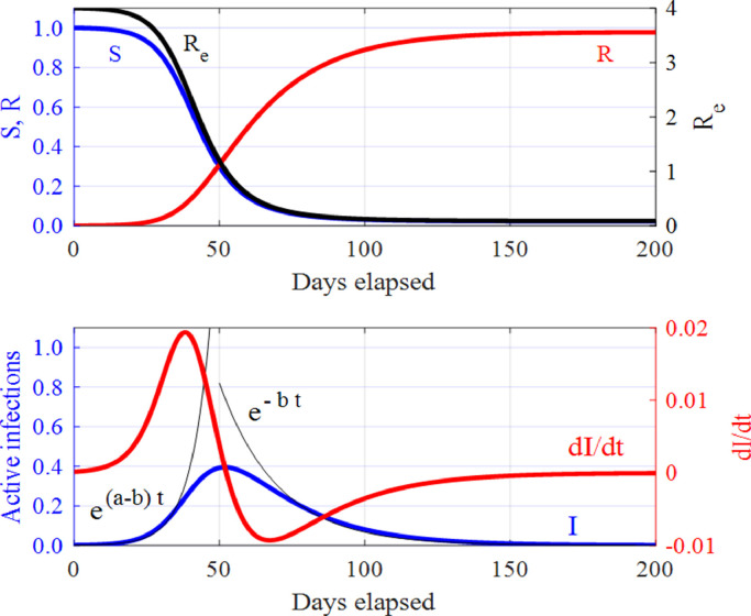
The evolution of the infected population is governed by the second ODE in system (1). In the beginning of the spread of an epidemic, where S ≈ 1, the number of infections increases exponentially $I=I\left(0\right)e^{(a-b)t}$. Then, the rate of infections falls to zero at the peak where $dI/dt=0$. When Sdrops below a certain level, the infected population decreases exponentially as $I\propto e^{-bt}$. A set of solutions is shown in Fig. 1 for a particular choice of initial conditions and model parameters, where one can see how the susceptible S, infected I, removed R, and effective reproduction number R_e, evolve in time. Next, we discuss the importance of R_e in the context of the virus spread as it can determine whether the disease will die out, continue to grow or the peak number of infections has been reached.

Fig. 1.

The SIR model (1): The time variation of the susceptible S, infected I and removed R populations, and of the effective reproduction number, R_e. The initial conditions and model parameters used here are: $S\left(0\right)=1,$$I\left(0\right)=0.001,$$R\left(0\right)=0,$$a=0.2$and $b=0.05$. The thin black curves correspond to the initial exponential growth $e^{(a-b)t}$and to the exponential decay $e^{-bt}$in the number of infected individuals I(t).

In particular, we can define the effective reproduction number R_e by $R_e=aS/b$. This is an important index as the evolution of the disease, in the absence of secondary peaks or surges, depends upon its value. When R_ebecomes less than one, the infected population decreases monotonically to zero, whereas when greater than one, it increases. Crucially, at $R_e=1,$the rate of increase of the infected population is zero, that corresponds to the peak number of active infected individuals. Thus, there is a critical value for the susceptible population, $S_C=b/a$. The number of active cases only declines when S < S_C. The reproduction number R_eand critical susceptibility S_C act as thresholds that determine whether an infectious disease will quickly die out or continue to grow. As the existence of a threshold for infection is not obvious from the data alone, it can be discerned from the properties of the SIR model (1), that makes it a powerful tool in understanding and predicting the spread of an epidemic.

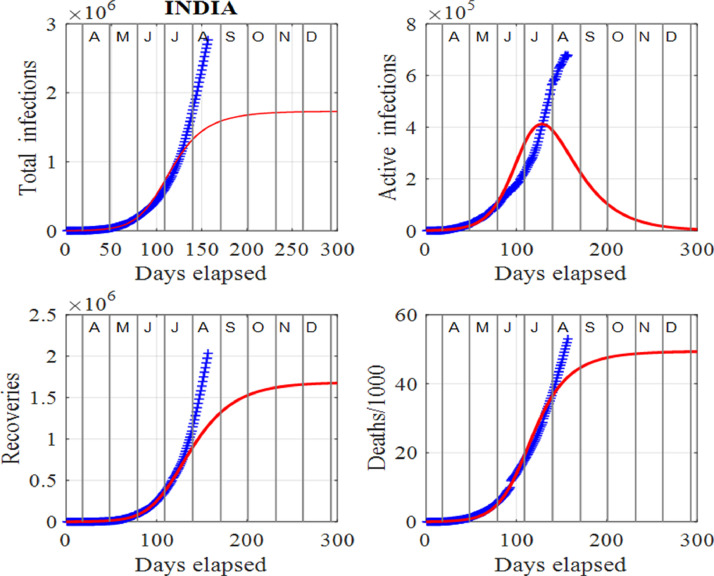
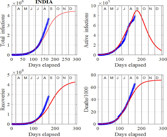
The rate of increase in the number of infections depends on the product of the number of infected and susceptible individuals. An understanding of system (1) explains the staggering increase in the infection rate around the world and currently, in India. The spread of the virus can only be contained when the number of susceptible individuals decreases with time. Our analysis shows that one cannot get accurate predictions by applying the SIR model (1) to the data for the pandemic in India. Fig. 2 identifies the problem in applying the SIR model to the Indian data starting on 14 March, 2020. The model and predictions are only in agreement at the start of the pandemic. The number of active infections in India does not reach a peak as it keeps getting bigger and bigger. However, modifying the SIR model by resetting the susceptible population at surge times, it is possible to fit the model predictions to the available published datasets [34]. Therefore, applying the SIR model to the Indian data augmented by the introduction of surge times in the susceptible population, one can make a quantitative analysis due to the spread of the virus in the country as we show in Sec. 4.

Fig. 2.

India: The SIR model predictions (14 March, 2020 to 8 January, 2021) and data (14 March, 2020 to 18 August, 2020) for the infections, recoveries and deaths. We note that the number of active infections does not reach a peak (see plot of active infections vs days elapsed), and keeps increasing in time. Thus, the solutions to the SIR model (1) and predictions are only in agreement at the start of the pandemic, i.e. the period for which the red (model solutions) and blue (published data in [34]) curves of the active infections are in good agreement.

3. Our modeling approach

In most countries, such as in India, there is not a homogenous mixing of the infected and susceptible individuals within the population, which is one of the strong assumptions in the standard SIR model. Only part of the total population will become susceptible to infected individuals. When infected individuals persist and move about within a community, further individuals may become susceptible to the disease. The susceptible population will not necessarily decrease monotonically with time. As susceptible individuals become infected, these new infections act as a source for more individuals to become susceptible. This gives rise to a positive feedback loop leading to a very rapid rise in the number of active infected cases in a surge period where the number of susceptible individuals increases instead of decreasing. Here, the SIR model (1) is considered in such a way that at any time t_s, the susceptible population can be reset to S_s(t_s), accommodating for secondary surges.

System (1) is solved for the variables S, I and R, where S, R and I ∈ [0, 1]. R and I are multiplied by a scaling factor f to give the number of individuals in each population group to match the model outputs with the published COVID-19 datasets in [34]. From now on, we consider in our analysis the scaled variables. Considering the solution for the removed population R, individuals can either recover or die, where C is the number of recoveries, D the number of deaths and $R=C+D$. The number of deaths, D, is estimated by fitting a function in the plot of the data for the number of actual deaths versus the data for the number of removals. We find that a good choice for the nonlinear function to estimate the number of deaths, Dfrom the number of removals R is

$$D=D_0\left(1-e^{-k_{0}R}\right).$$ (2)

If new outbreaks occur, then the death rate can suddenly increase again at time t and the number of deaths is given by

$$D=D_t+D_1\left(1-e^{-k_{1}R}\right)$$ (3)

where D ₀, D ₁, D_t, k ₀ and k ₁ are constants suitably selected to give the best-fit (by visual inspection) between the function and the data. Although this is subjective, we have checked that it may be a better approach than using an automated optimization program for calculating the input parameters due to the nature of the recorded data. We note here that Eq. (3) was only used for the deaths in Iran as shown in Fig. 12. The number of recoveries, C is then simply given by $C=R-D$.

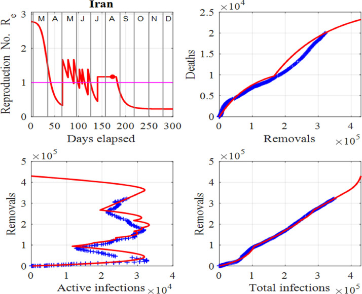
Fig. 12.

Iran: Effective reproduction number Re as a function of time, deaths against removals, removals against active infections and removals against cumulative total infections. The red dot represents the value of R_e for the last day in the data. Also, the horizontal line in the first panel shows the critical case where $R_e=1$and in the last three panels, the red curves are those from the model solutions and the blue from the published data in [34].

The model input parameters are the population scaling factor f, the initial infected population I(0), the initial removed population R(0), the rate constants a and b, death constants D ₀, D ₁, D_t, k ₀ and k ₁, and the surge periods t_s and S_s. This set of constants is appropriately considered to best-fit the model predictions with the datasets [34] for each country in our study. As new data become available, a small amount of adjustment to the input parameters in model (1) can be made to get a better agreement between the model predictions and the data. Model (1) cannot predict the time and height of the peak in the number of active infections. However, if the number of active infections keeps increasing, S can be increased which has the effect on increasing the peak value for active infections and delaying the time at which the peak will occur. The adjustments that are necessary to reset the value of S are an important indicator of the success or failure of government actions in controlling the spread of the virus. High values of resetting of S or a high reset frequency indicates that the spread of the virus is not contained in the community. Only when the susceptible population decreases towards zero, the number of active infections declines to zero. As we show in Sec. 4, although the peak for active infections has not been reached in India, the model augmented by the introduction of surges as proposed here, gives the estimates of the duration of the pandemic and minimum estimates for the total cumulative number of infections and deaths, that allows for valuable forecasts and informed decisions to confine the spread of the virus.

4. Results

Data have been collected from [34] for Italy, India, South Korea and Iran until August, 2020. The system of Eqs. (1) was solved using the fourth order Runge-Kutta method. The model predictions and data for each country are displayed graphically for a period of 300 days, which amounts to the period from March, 2020 to December, 2021. The crosses are for the published datasets in [34] and the smooth lines for the results from our methodology. The adjustable model input parameters are: the population scaling factor f, the initial number of infections I(0), the initial number of removals R(0), the transmission rate constant a, the removal rate constant b, and constants D ₀, D ₁, D_t, k ₀ and k ₁ to calculate the number of deaths from the number of removals R from the published data in [34]. The results of our study are then shown in Figs. 2 to 12. The time evolution figures show the cumulative total number of infections, I_tot, the active cases, I, recoveries, C, deaths, D and the effective reproduction number, R_e. The red dot gives the value of R_e for the last day in the data. The figures for the deaths, D against removals, R are used to find the parameters in function (2) that best describes the relationship between D and R. The figures of removals, R against total infections, I_tot are useful for fitting the input parameters and may be useful as indicators of a change in trend or the peak in the number of active cases. The plots of removals, R against the number of active infections, I are also useful for fitting the input parameters and for identifying peaks in active infections and changes in trends. The input parameters are adjusted by visual inspection to incorporate suitable values corresponding to the best fit of the model predictions to the published data. As we have checked, it may be possible to use an optimization program to fit the parameters, however, we found out that it will not necessarily improve the predictions in tracking the data due to the quality of the recorded data.

We start by analysing the data from Italy and then move on to the studies of the datasets from India, South Korea, and Iran.

4.1. Italy

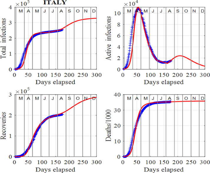
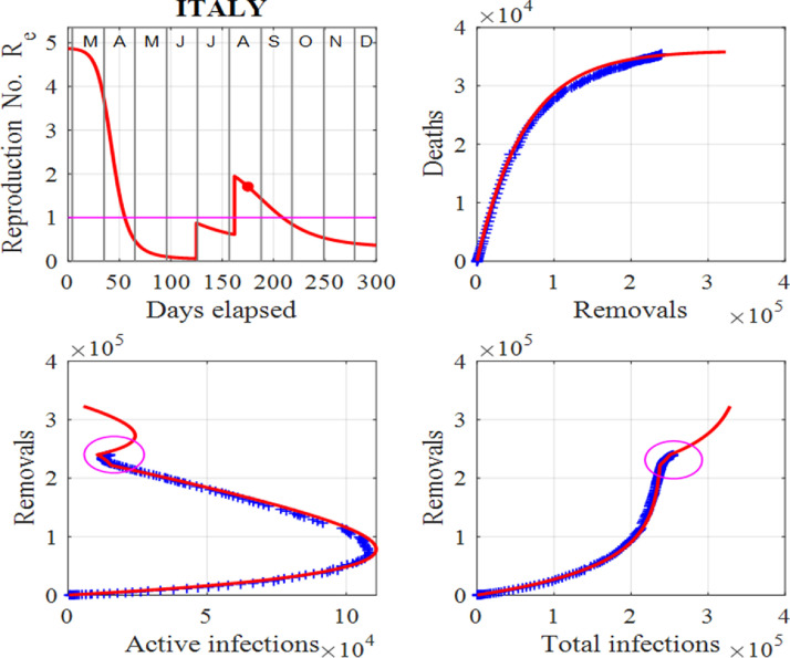
Figs. 3 and 4 show our modelling results for the data from Italy. The virus has left a trail of suffering throughout the country, especially in the northern regions. Italy was the first country in Europe to suffer severe effects of the virus [4], [5], [10], [12], [14]. The numbers of infections and deaths increased very rapidly from mid March, 2020 until the end of April, 2020. This led to hospitals being quickly overwhelmed and the government imposed a strict lockdown for two months. The lockdown period was very successful with the peak infections of about 108000 occurring around 20 April, 2020 and the susceptible population falling below the critical value $R_e=1,$indicated by the horizontal line in the first panel in Fig. 4. Since the peak, the number of active infections has consistently decreased as predicted by the model until August, 2020, as Figs. 3 and 4 show a discontinuation of this downward trend in active infections. As of early August, 2020, the effective reproduction number has been reset to a number greater than one. Fitting the model to the data predicts only a small increase in the number of active infections. However, by tracking the data with the model daily, the surge factor, S can easily be updated to give a more informed projection of the future number of infections. In all figures for Italy, our approach has been able to track the published data [34] exceedingly well. Also, the relationship between deaths and removals is very well described by Eq. (2). This initial sharp rise in deaths and then taping off in the number of deaths as the number of removals increases, is a very common trend observed in other countries studied herein.

Fig. 3.

Italy: Time evolution of the populations of cumulative total infections, active infections, recoveries and deaths/1000. The input parameters used in the modelling are the following: $I\left(0\right)=1.3\times {10}^{-3},$$R\left(0\right)=6.21\times {10}^{-4},$$f=2.4\times {10}^5,$$a=0.18,$$b=0.037,$$D_0=3.6\times {10}^4$and $k_0=1.6\times {10}^{-5}$. We note that the red curves are those from the model solutions and the blue from the published data in [34].

Fig. 4.

Italy: Effective reproduction number R_e as a function of time, deaths against removals, removals against active infections and removals against cumulative total infections. The red dot represents the value of R_e for the last day in the data in [34] and the ellipses depict the changes in trends, which indicate the start of a surge. We note that the horizontal line in the first panel shows the critical case where $R_e=1$and in the last three panels, the red curves are those from the model solutions and the blue from the published data in [34].

In early May, 2020, people were allowed to move within their regions to visit family provided they wear face masks, and some parks were reopened for exercise. Slowly, restrictions are being lifted in the country. Manufacturers and construction firms have resumed work and shops are starting reopening. There has been no need to apply any surges in the susceptible population and this is a strong indicator that so far the lifting of the restrictions has not faulted the downward spiral in the number of active infections until July, 2020. By the end of June, 2020, the actions taken by the Italian government have succeeded in controlling the spread of the virus and infections have been seen to decrease continuously.

However, as of early August, 2020, the downward trend has ceased. How large this spike in infections will be, will depend directly upon actions taken by the Italian authorities and individuals. The model cannot accurately predict how the number of infections will increase, however different scenarios can be considered. For example, if the susceptible population was held constant for a week in early August, 2020, instead of the simple spike as shown in Fig. 4 indicated by the ellipses, then the number of active infections would double. This shows that the virus can easily get out of control leading to a very significant increase in infections. If governments and individuals do not take actions immediately, an uptrend in infections results. The model is useful in the early identification of this change in trend by considering the plots of removals against infections rather than the published data, as indicated by the ellipses in Fig. 4.

We can explain the reasons for the large number of infections and deaths in Italy with insights gained from the SIR model (2). There is strong evidence that in December, 2019 people were already infected, although the first reported case of an infected individual was not until 31 January, 2020. The rate of change of the infections depends upon the number of infections and the number of susceptible individuals as given by system (1). During December, 2019, and January, 2020, the infected individuals, many of them asymptomatic, led to an increase in the susceptible population. Thus, from a starting point with a low number, the number of infections ballooned rapidly, following initially an exponential increase. The recorded number of active cases was 1049 on 29 February, 2020, 2262 on 3 March, 2020 and 10578 on 11 March, 2020. The numbers of infections and deaths caused by the pandemic have been huge in Italy. However, by the end of June, 2020, the actions taken by the government have succeeded in controlling the death rate. Eqn. 2 describes the relationship between deaths and removals very well and this is shown in Fig. 4 (see plot for the deaths vs removals).

Governments and their advisors around the world often stated no urgent actions are required as long as the active case numbers are low, but this is actually the time when actions need to be taken as the initial increase of the spread follows an exponential increase, as seen in model (1)! The Italian government was not fully aware of the presence of the virus early in 2020, hence it did not take the necessary control measures to control its spread. For example, compare the spread of the virus in Italy and South Korea. The South Korean government took immediate actions in January and February, 2020 to control the virus and near the end of August, 2020, there has been only 306 deaths and less than 14000 total infections. This is probably due to the fact that South Korea has a transparent and open system of government that has managed the crisis with relatively few deaths and infections. Authorities took a proactive approach to testing, contact tracing, treatment and isolation, expedited by its world-leading technological capabilities and public healthcare system.

4.2. India

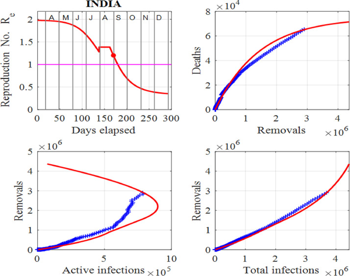
Figs. 5 and 6 show the estimates from the data and the model predictions (1) for India. Clearly, as of mid August, 2020, the spread of the virus throughout the country is not being contained and the peak number of active cases may be a long way into the future. The infected population is still increasing and a peak in the active infections has not yet been attained, as shown in Fig. 5. The model is designed so that the model’s predictions track the published data in [34]. Hence, the model cannot predict the peak number of active cases in the future. However, by adding surges, the peak can be delayed and increased. Although the selection of model’s input parameters and surge times are subjective, the data can be tracked quite successfully and can give estimates of the populations in the future and possible time scales for the number of active cases to drop to low values, that allows for valuable predictions. India is caught in a vicious positive feedback loop like the USA. New infections result in an increase in the susceptible population as the disease spreads. Consequently, these individuals may become infected and the cycle continues. This cycle is difficult to terminate, resulting in the number of infections getting larger and larger. One of the major methods in controlling the increase of infections is to test, contact trace and quarantine. However, when there is such large numbers of infections as in India, this method is not practical.

Fig. 5.

India: Time evolution of the populations of cumulative total infections, active infections, recoveries and deaths/1000. The input parameters are as follows: $I\left(0\right)={10}^{-3},$$R\left(0\right)=5\times {10}^{-6},$$f=4\times {10}^6,$$a=0.085,$$b=0.043,$$D_0=7.5\times {10}^4$and $k_0=7\times {10}^{-7}$. We note that the red curves are those from the model solutions and the blue from the published data in [34]. Also, note the absence of peaks, that shows the published data departed from the model solutions.

Fig. 6.

India: Effective reproduction number R_e as a function of time, deaths against removals, removals against active infections and removals against cumulative total infections. We note that the red dot represents the value of R_e for the last day in the data, the horizontal line in the first panel shows the critical case where $R_e=1$and in the last three panels, the red curves are those from the model solutions and the blue from the published data in [34].

Fig. 6 shows that the peak in the number of active cases may not occur for some time. The observation of the susceptible variable, S shows that the susceptible population has to be repeatedly reset to higher values. This is a strong indicator that the spread of the virus is not contained in the country. The plots for the removals against infections or total infections show that the data has not reached the knee section of the model’s prediction again, providing evidence that the peak in the active infections may not occur any time soon. It is most likely that in the near future, there will be an alarming increase in the number of new infections and deaths in India. The model predictions make it possible to consider many of the scenarios that may result.

4.3. South Korea

South Korea has a transparent and open system of government that has managed the crisis with relatively few deaths and infections. Authorities took a proactive approach to testing, contact tracing, treatment and isolation, expedited by its world-leading technological capabilities and public healthcare system. Lives for many in South Korea have more or less rolled on as usual. It is mandatory to wear masks on public transport and most South Koreans wear masks when going out. South Korea has tried to remain as open as possible by responding proportionally to the scientific assessments of the risks.

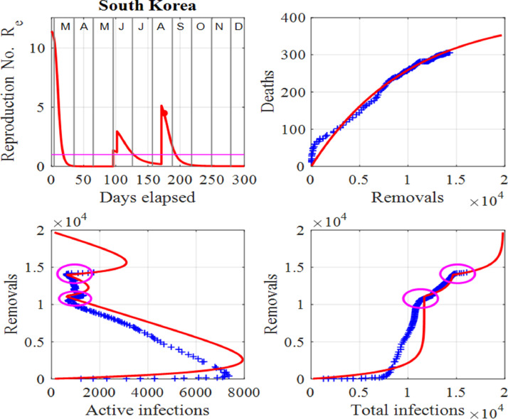
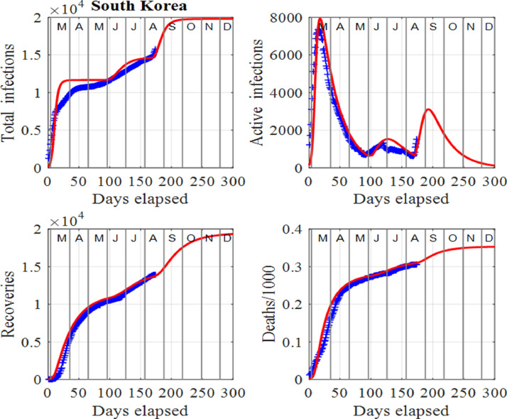
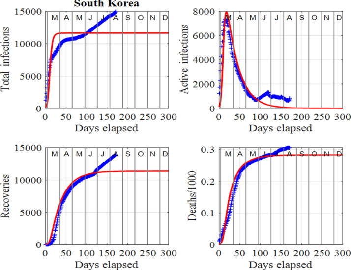
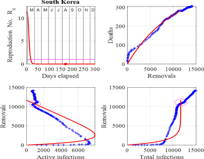
One can identify a change of a trend in infections when there is a departure between the trajectories of the published data and model predictions before a surge is applied to the model. The disparity between the published data and model predictions can be used as an early warning sign of a new outset of the virus in the community as indicated by the ellipses in Fig. 8 for South Korea. Changes in trends occurred at the beginning of June, 2020, and another in mid August, 2020. The spike in active number of infections in June, 2020 may have been due to new clusters of infections as a result of clubs and bars reopening. In this instance, South Korean authorities acted swiftly by isolating some areas, testing and contact tracing and some schools were forced to close just days after reopening. The result was only a small spike in active infections occurring at the beginning of July, 2020. The second surge occurring in mid August, 2020 appears to be much more serious since a large surge factor had to be applied in the model to match the published data and model predictions. Figs. 7 and 8 show the graphical comparisons between the data and model predictions when surge periods are included, whereas Figs. 9 and 10 show the predictions if no surges were applied. Table 1 summarizes some of these predictions.

Fig. 8.

South Korea: Effective reproduction number R_e as a function of time, deaths against removals, removals against active infections and removals against cumulative total infections. The red dot represents the value of R_e for the last day in the data and the ellipses depict the changes in trends, which indicate the start of two surges. Also, the horizontal line in the first panel shows the critical case where $R_e=1$and in the last three panels, the red curves are those from the model solutions and the blue from the published data in [34].

Fig. 7.

South Korea: Time evolution of the populations of cumulative total infections, active infections, recoveries and deaths/1000. The input parameters are as follows: $I\left(0\right)=1.2\times {10}^{-2},$$R\left(0\right)=3.13\times {10}^{-3},$$f=1.15\times {10}^4,$$a=0.4,$$b=0.035,$$D_0=400$and $k_0={10}^{-4}$. We note that the red curves are those from the model solutions and the blue from the published data in [34].

Fig. 9.

South Korea: Time evolution of the populations of cumulative total infections, active infections, recoveries and deaths/1000 when surges have not been applied. The red curves are those from the model solutions and the blue from the published data in [34].

Fig. 10.

South Korea: Effective reproduction number R_e as a function of time, deaths against removals, removals against active infections and removals against cumulative total infections when surges have not been applied. The red dot represents the value of R_e for the last day in the data and the ellipses depict the changes in trends, which indicate the start of a surge. Also, the horizontal line in the first panel shows the critical case where $R_e=1$and in the last three panels, the red curves are those from the model solutions and the blue from the published data in [34].

Table 1.

South Korea: Predictions for 22 December, 2020 for the cumulative total number of infections, I_tot, active cases, I, recoveries, C and deaths, D when surges are included (second row) and no surges applied (third row). In brackets, we report the percentages of the corresponding populations.

South Korea	Itot	I	C	D
Surges	19797	121 (0.6%)	19323 (97.6%)	353 (1.8%)
No surges	11674	1 (0.0%)	11391 (97.6%)	282 (2.4%)

4.4. Iran

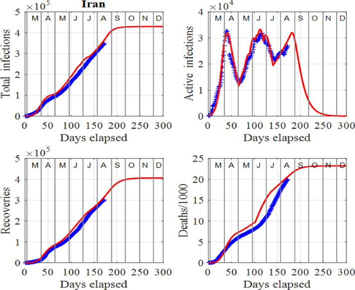
Iran is one of the worst-hit countries in the Middle East and started easing its lockdown in April, 2020, after a drop in the number of deaths. As a result, a second wave of infections peaked in mid June, 2020, with a peak height similar to the first. In July, 2020, the number of infections started to decrease again. However, a third wave of infections has started developing in August, 2020. Figs. 11 and 12 highlight the dangers ahead for Iran. Since the beginning of July, 2020, the number of deaths has risen rapidly and with little tapping off in the death rate.

Fig. 11.

Iran: Time evolution of the populations of cumulative total infections, active infections, recoveries and deaths/1000. The input parameters are as follows: $I\left(0\right)=2\times {10}^{-3},$$R\left(0\right)=0,$$f=1.2\times {10}^5,$$a=0.25,$$b=0.09,$$D_0=1.2\times {10}^4,$$k_0={10}^{-5},$$D_t=9.7217\times {10}^3,$$D_1=16\times {10}^3$and $k_1=6\times {10}^{-6}$. We note that the red curves are those from the model solutions and the blue from the published data in [34].

The analysis shows that the number of deaths and infections will continue to increase, unless governments and individuals take actions to prevent people becoming susceptible. To track the data for Iran, a number of surges in the susceptible population, S are necessary. Resetting S is very subjective, however, the numbers used are not as important as the fact that the susceptible population is increasing, and when this occurs, the spread of the virus is out of control and thus, the number of infections will continually increase.

5. Conclusions

How the virus spreads in a community is a complex issue, affected by a multitude of factors. In this paper, the proposed approach is designed to remove many of these complexities and yet to be useful in both quantitative and qualitative ways. This is accomplished by including surge periods where the susceptible population can be reset to larger numbers allowing for the tracking of the published datasets where new clusters of infections occur in the community. The frequency at which surge periods are needed to be applied and their magnitudes, are good indicators that the spread of the virus is not under control in the community. Although the SIR model cannot predict the severity and time of the peak in the active infections, the peak in the number of active infections and the number of deaths, it does give minimum estimates for the duration of the virus, the total cumulative number of infections, the peak in the number of active infections and the number of deaths. The model and approach used here may be a useful tool in detecting the early onset of further waves of infections allowing governments and authorities to take appropriate measures to contain them.

The methodology presented here suggests there is a possibility of a spike or second wave of infections coming soon in Italy. In India, the number of infections keeps rising and the model only gives minimum estimates of infections, deaths and time scales for the evolution of the virus. Our analysis suggests that a small spike that occurred at the end of June, 2020, in South Korea, may be followed by another spike in August, 2020. According to our results, the virus is something that will not go away. Many people assume that when the number of active infections starts to decrease, life can get back to normal. This is far from the truth as shown by the application of the presented methodology to the published data for Iran. The first wave in Iran peaked in early April, 2020, and the second in mid June, 2020. However, there is a possibility of a spike or even a third wave in Iran starting towards the end of August, 2020.

The virus has severely impacted all aspects of people’s lives around the world for more than seven months now [12], [21]. Typically, the half-life for the decrease in active cases is around 18 days. For India, even if the peak in active cases occurred at the end of August, 2020, and there were no further surges, then by January, 2021 there would still be about 100000 active cases. Even after a peak, there is a considerable probability that there will be periods when the number of infections spike again as in Iran and South Korea. Therefore, it is imperative that governments and individuals do not assume that the virus is going away and maintain or even increase measures that have been confirmed to prevent individuals becoming susceptible to the disease. Only as the susceptible population converges to zero, the number of active cases goes to zero. If reliable, recorded data are available, our methodology provides an effective tool to track the spread of the virus and insights into the management of the control measures implemented by governments and local authorities. In this paper, our methodology has been applied to published data from Italy, India, South Korea and Iran. A strength of our methodology lies in the fact that as new data are added daily, the model parameters are easy to adjust and provide the best-fit curves between the data and the model predictions. By comparing the published data with the model predictions, it is possible to reach conclusions based upon science about the effectiveness of control and adequate measures implemented by governments, local authorities and people within communities.

Finally, for the virus to be controlled and to limit its impact on society, various governments have imposed drastic actions to prevent people from becoming susceptible to the disease. Some actions that are proving to be successful include: total lockdowns, testing, contact tracing of people who may have been in contact with an infected individual and then isolating them, isolating suspected individuals, restrictions on the movement of people, restrictions on large gatherings, hygiene measures such as washing hands, and wearing face masks particularly on public transport or in crowded indoor spaces. By using the predictions of mathematical modeling and comparing it with published data, as we did here, one is more able to assess actions that have been taken to control the spread of the virus. Such advanced policies and strategies are needed to overcome the situation. Researchers across different disciplines have been working to deal with this pandemic by providing novel approaches, optimal policies, mathematical methods for predictions, biological phenomena and drugs to mitigate the effects [12], [38], [39], [40], [41], [42]. Our analysis shows that one thing is certain: COVID-19 is not going to go way quickly or easily.

Credit author Statement

Ian Cooper: designed the work, worked on the numerical results and contributed to draft preparation. Argha Mondal: contributed to designing the work and to preparing the manuscript with analytical and numerical support. Chris G. Antonopoulos: contributed to writing, reviewing and editing the manuscript with constructive suggestions.

Declaration of Competing Interest

The authors declare that they have no known competing financial interests or personal relationships that could have appeared to influence the work reported in this paper.

References

- 1.World health organization, coronavirus disease (COVID-19) outbreak. https://www.who.int/emergencies/diseases/novel-coronavirus-2019.
- 2.Boccaletti S., Ditto W., Mindlin G., Atangana A. Vol. 135. Chaos, Solitons & Fractals; 2020. Modeling and forecasting of epidemic spreading: The case of COVID-19 and beyond; p. 109794. [DOI] [PMC free article] [PubMed] [Google Scholar]
- 3.Wu J.T., Leung K., Leung G.M. Nowcasting and forecasting the potential domestic and international spread of the 2019-ncov outbreak originating in wuhan. China: a modelling study The Lancet. 2020;395(10225):689–697. doi: 10.1016/S0140-6736(20)30260-9. [DOI] [PMC free article] [PubMed] [Google Scholar]
- 4.World health organization. 2020. Coronavirus disease (COVID-19): situation reports, https://www.who.int/emergencies/diseases/novel-coronavirus-2019/situation-reports/?gclid=CjwKCAjwltH3BRB6EiwAhj0IUO8zXPbywCzIK6R33ZdImpSd-V-wRyfdY-UA8XDue1rTxITc8M07rxoCxCsQAvD_BwE.
- 5.Remuzzi A., Remuzzi G. COVID-19 and italy: what next? The Lancet. 2020;395(10231):1225–1228. doi: 10.1016/S0140-6736(20)30627-9. [DOI] [PMC free article] [PubMed] [Google Scholar]
- 6.Sohrabi C., Alsafi Z., O’Neill N., Khan M., Kerwan A., Al-Jabir A., Iosifidis C., Agha R. World health organization declares global emergency: A review of the 2019 novel coronavirus (COVID-19) Int J Surg. 2020;76:71–76. doi: 10.1016/j.ijsu.2020.02.034. [DOI] [PMC free article] [PubMed] [Google Scholar]
- 7.Liu Y., Yan L.M., Wan L., Xiang T.X., Le A., Liu J.M., Peiris M., Poon L.L.M., Zhang W. Viral dynamics in mild and severe cases of COVID-19. The Lancet Infectious Diseases. 2020;20(6):656–657. doi: 10.1016/S1473-3099(20)30232-2. [DOI] [PMC free article] [PubMed] [Google Scholar]
- 8.Anderson R.M., Heesterbeek H., Klinkenberg D., Hollingsworth T.D. How will country-based mitigation measures influence the course of the COVID-19 epidemic? The Lancet. 2020;395(10228):931–934. doi: 10.1016/S0140-6736(20)30567-5. [DOI] [PMC free article] [PubMed] [Google Scholar]
- 9.Kraemer M.U.G., Yang C.H., Gutierrez B., Wu C.H., Klein B., Pigott D.M., du Plessis L., Faria N.R., Li R., Hanage W.P., Brownstein J.S., Layan M., Vespignani A., Tian H., Dye C., Pybus O.G., Scarpino S.V. The effect of human mobility and control measures on the COVID-19 epidemic in china. Science. 2020;368(6490):493–497. doi: 10.1126/science.abb4218. [DOI] [PMC free article] [PubMed] [Google Scholar]
- 10.Fanelli D., Piazza F. Analysis and forecast of COVID-19 spreading in china. Italy and France Chaos, Solitons & Fractals. 2020;134:109761. doi: 10.1016/j.chaos.2020.109761. [DOI] [PMC free article] [PubMed] [Google Scholar]
- 11.Xue L., Jing S., Miller J.C., Sun W., Li H., Guillermo Estrada-Franco J., Hyman J.M., Zhu H. Toronto and Italy. Mathematical Biosciences; 2020. A data-driven network model for the emerging COVID-19 epidemics in Wuhan; p. 108391. [DOI] [PMC free article] [PubMed] [Google Scholar]
- 12.Giordano G., Blanchini F., Bruno R., Colaneri P., Di Filippo A., Di Matteo A., Colaneri M. Modelling the COVID-19 epidemic and implementation of population-wide interventions in italy. Nat. Med. 2020:1–6. doi: 10.1038/s41591-020-0883-7. [DOI] [PMC free article] [PubMed] [Google Scholar]
- 13.Kucharski A.J., Russell T.W., Diamond C., Liu Y., Edmunds J., Funk S., Eggo R.M. Early dynamics of transmission and control of COVID-19: a mathematical modelling study. The Lancet Infectious Diseases. 2020 doi: 10.1016/S1473-3099(20)30144-4. [DOI] [PMC free article] [PubMed] [Google Scholar]
- 14.Livingston E., Bucher K. Coronavirus disease 2019 (COVID-19) in italy. Jama. 2020;323(14) doi: 10.1001/jama.2020.4344. [DOI] [PubMed] [Google Scholar]; 1335–1335
- 15.Scarpino S.V., Petri G. On the predictability of infectious disease outbreaks. Nat. Commun. 2019;10(1):1–8. doi: 10.1038/s41467-019-08616-0. [DOI] [PMC free article] [PubMed] [Google Scholar]
- 16.Dziugys A., Bieliunas M., Skarbalius G., Misiulis E., Navakas R. Simplified model of covid-19 epidemic prognosis under quarantine and estimation of quarantine effectiveness. Chaos, Solitons & Fractals. 2020;140:110162. doi: 10.1016/j.chaos.2020.110162. [DOI] [PMC free article] [PubMed] [Google Scholar]
- 17.Chinazzi M., Davis J.T., Ajelli M., Gioannini C., Litvinova M., Merler S., Pastore P.A., Mu K., Rossi L., Sun K., Viboud C., Xiong X., Yu H., Halloran M.E., Longini I.M., Vespignani A. The effect of travel restrictions on the spread of the 2019 novel coronavirus (COVID-19) outbreak. Sci. 2020;368(6489):395–400. doi: 10.1126/science.aba9757. [DOI] [PMC free article] [PubMed] [Google Scholar]
- 18.Pai C., Bhaskar A., Rawoot V. Investigating the dynamics of COVID-19 pandemic in india under lockdown. Chaos, Solitons & Fractals. 2020;138:109988. doi: 10.1016/j.chaos.2020.109988. [DOI] [PMC free article] [PubMed] [Google Scholar]
- 19.Ndairou F., Area I., Nieto J.J., Torres D.F. Mathematical modeling of COVID-19 transmission dynamics with a case study of wuhan. Chaos, Solitons & Fractals. 2020:109846. doi: 10.1016/j.chaos.2020.109846. [DOI] [PMC free article] [PubMed] [Google Scholar]
- 20.Li Q., Tang B., Bragazzi N.L., Xiao Y., Wu J. Modeling the impact of mass influenza vaccination and public health interventions on COVID-19 epidemics with limited detection capability. Math. Biosci. 2020:108378. doi: 10.1016/j.mbs.2020.108378. [DOI] [PMC free article] [PubMed] [Google Scholar]
- 21.Anastassopoulou C., Russo L., Tsakris A., Siettos C. Data-based analysis, modelling and forecasting of the COVID-19 outbreak. PLOS ONE. 2020;15(3) doi: 10.1371/journal.pone.0230405. [DOI] [PMC free article] [PubMed] [Google Scholar]; E0230405
- 22.Postnikov E.B. Estimation of COVID-19 dynamics “on a back-of-envelope”: does the simplest SIR model provide quantitative parameters and predictions? Chaos, Solitons & Fractals. 2020;135:109841. doi: 10.1016/j.chaos.2020.109841. [DOI] [PMC free article] [PubMed] [Google Scholar]
- 23.Peng L., Yang W., Zhang D., Zhuge C., Hong L.. Epidemic analysis of COVID-19 in china by dynamical modeling. 2020. 10.1101/2020.02.16.20023465
- 24.Wangping J., Ke H., Yang S., Wenzhe C., Shengshu W., Shanshan Y., Jianwei W., Fuyin K., Penggang T., Jing L., Miao L., Yao H. Extended SIR prediction of the epidemics trend of COVID-19 in italy and compared with hunan, china. Frontiers in Medicine. 2020;7:169. doi: 10.3389/fmed.2020.00169. [DOI] [PMC free article] [PubMed] [Google Scholar]
- 25.Shim E., Tariq A., Choi W., Lee Y., Chowell G. Transmission potential and severity of COVID-19 in south korea. Int. J. Infect. Dis. 2020;93:339–344. doi: 10.1016/j.ijid.2020.03.031. [DOI] [PMC free article] [PubMed] [Google Scholar]
- 26.Liu Z., Magal P., Seydi O., Webb G.. A model to predict COVID-19 epidemics with applications to south korea, italy, and spain. 2020b. 10.1101/2020.04.07.20056945. [DOI]
- 27.Ghanbari B. On forecasting the spread of the COVID-19 in iran: The second wave. Chaos, Solitons & Fractals. 2020;140:110176. doi: 10.1016/j.chaos.2020.110176. [DOI] [PMC free article] [PubMed] [Google Scholar]
- 28.India under COVID-19 lockdown, The Lancet, 395(10233), 1315, 10.1016/S0140-6736(20)30938-7 [DOI] [PMC free article] [PubMed]
- 29.Hethcote H.W. Springer; 1989. Three basic epidemiological models. In Applied mathematical ecology. [Google Scholar]
- 30.Hethcote H.W. The mathematics of infectious diseases. SIAM Review. 2000;42(4):599–653. [Google Scholar]
- 31.Hethcote H.W. The basic epidemiology models: models, expressions for r0, parameter estimation, and applications. In Mathematical Understanding of Infectious Disease Dynamics. 2009;16:1–61. [Google Scholar]
- 32.Weiss H.H. The SIR model and the foundations of public health. MATerials MATemàtics. 2013:1–17. [Google Scholar]
- 33.Cooper I., Mondal A., Antonopoulos C.G. A SIR model assumption for the spread of COVID-19 in different communities. Chaos, Solitons & Fractals. 2020;139:110057. doi: 10.1016/j.chaos.2020.110057. [DOI] [PMC free article] [PubMed] [Google Scholar]
- 34.Coronavirus worldometer website. https://www.worldometers.info/coronavirus/.
- 35.COVID-19 INDIA. https://www.mohfw.gov.in/.
- 36.Sardar T., Nadim S.S., Rana S., Chattopadhyay J. Assessment of lockdown effect in some states and overall india: A predictive mathematical study on COVID-19 outbreak. Chaos, Solitons & Fractals. 2020;139:110078. doi: 10.1016/j.chaos.2020.110078. [DOI] [PMC free article] [PubMed] [Google Scholar]
- 37.Sarkar K., Khajanchi S., Nieto J.J. Modeling and forecasting the COVID-19 pandemic in india. Chaos, Solitons & Fractals. 2020;139:110049. doi: 10.1016/j.chaos.2020.110049. [DOI] [PMC free article] [PubMed] [Google Scholar]
- 38.Zhao H., Feng Z. Staggered release policies for COVID-19 control: Costs and benefits of relaxing restrictions by age and risk. Math. Biosci. 2020:108405. doi: 10.1016/j.mbs.2020.108405. [DOI] [PMC free article] [PubMed] [Google Scholar]
- 39.Rüdiger S., Plietzsch A., Sagués F., Sokolov I.M., Kurths J. Epidemics with mutating infectivity on small-world networks. Sci. Reps. 2020;10(1):1–11. doi: 10.1038/s41598-020-62597-5. [DOI] [PMC free article] [PubMed] [Google Scholar]
- 40.Feng Z., Glasser J.W., Hill A.N. On the benefits of flattening the curve: A perspective. Math. Bioscis. 2020:108389. doi: 10.1016/j.mbs.2020.108389. [DOI] [PMC free article] [PubMed] [Google Scholar]
- 41.Cakan S. Dynamic analysis of a mathematical model with health care capacity for pandemic COVID-19. Chaos, Solitons & Fractals. 2020;139:110033. doi: 10.1016/j.chaos.2020.110033. [DOI] [PMC free article] [PubMed] [Google Scholar]
- 42.Bjørnstad O.N., Shea K., Krzywinski M., Altman M. Modeling infectious epidemics. Nature Methods. 2020;17:455–456. doi: 10.1038/s41592-020-0822-z. [DOI] [PubMed] [Google Scholar]