Abstract
In this paper, a novel approach called GSA-DenseNet121-COVID-19 based on a hybrid convolutional neural network (CNN) architecture is proposed using an optimization algorithm. The CNN architecture that was used is called DenseNet121, and the optimization algorithm that was used is called the gravitational search algorithm (GSA). The GSA is used to determine the best values for the hyperparameters of the DenseNet121 architecture. To help this architecture to achieve a high level of accuracy in diagnosing COVID-19 through chest x-ray images. The obtained results showed that the proposed approach could classify 98.38% of the test set correctly. To test the efficacy of the GSA in setting the optimum values for the hyperparameters of DenseNet121. The GSA was compared to another approach called SSD-DenseNet121, which depends on the DenseNet121 and the optimization algorithm called social ski driver (SSD). The comparison results demonstrated the efficacy of the proposed GSA-DenseNet121-COVID-19. As it was able to diagnose COVID-19 better than SSD-DenseNet121 as the second was able to diagnose only 94% of the test set. The proposed approach was also compared to another method based on a CNN architecture called Inception-v3 and manual search to quantify hyperparameter values. The comparison results showed that the GSA-DenseNet121-COVID-19 was able to beat the comparison method, as the second was able to classify only 95% of the test set samples. The proposed GSA-DenseNet121-COVID-19 was also compared with some related work. The comparison results showed that GSA-DenseNet121-COVID-19 is very competitive.
Keywords: SARS-CoV-2, Deep learning, Convolutional neural networks, Transfer learning, Gravitational search algorithm, Hyperparameters optimization
Graphical abstract

Highlights
-
•
An optimized deep learning DenseNet121 architecture for the diagnosis of COVID-19 disease is proposed.
-
•
The gravitational search optimization (GSA) algorithm was used to select the optimal values for the hyperparameters of the DenseNet121 architecture.
-
•
The GSA-DenseNet121-COVID-19 performance was compared to the performance of a CNN architecture called Inception-v3.
-
•
The proposed approach achieves a 98% accuracy on the test set.
1. Introduction
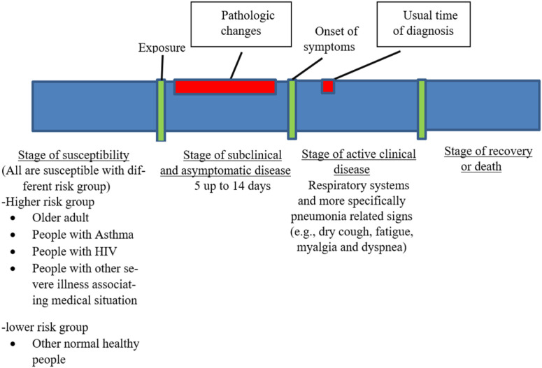
On 11/March/2020, the world health organization (WHO) announced that the novel coronavirus disease-2019 (COVID-19) had been a Pandemic outbreak. COVID-19 is a respiratory disease caused by severe acute respiratory syndrome coronavirus 2 (SARS-CoV-2). SARS-CoV-2 is a virus that belongs to the Coronavirdeae family, which is the same family of both severe acute respiratory syndrome coronavirus and middle east respiratory syndrome coronavirus (MERS-CoV) [1]. Both SARS-CoV-1 and MERS-CoV are the 2002 severe acute respiratory syndrome causative agent and the 2012 middle east respiratory syndrome MERS epidemic [2], [3]. This announcement was the beginning of the current medical health problem faced and shared by the whole world during the last few months. Up till now, there are no efficient protective vaccines, neutralizing antisera or curative medication have been developed or officially approved to be used in COVID-19’s patients worldwide. The continuous increase in morbidities and mortalities due to SARS-CoV-2 leads to international medical health worsen situations day after day. Therefore, this emerging COVID-19 pandemic becomes an ongoing challenge for all medical health workers and researchers, by applying the natural timeline of infectious diseases [4] on COVID-19, as shown in Fig. 1. The importance of shortening the period between the onset of symptoms and the usual diagnosis will appear. Therefore, an efficient rapid diagnostic test or protocol will help to achieve proper early medical caring to COVID-19 patients that, by its role, will help to save a lot of lives worldwide. Finding a rapid, efficient diagnostic test or protocol becomes one of those top critical priorities.
Fig. 1.
Natural timeline of infectious diseases on COVID-19.
Adapted from [4].
Quantitative reverse transcriptase-polymerase chain reaction (qPCR) is the golden standard test for confirmed laboratory diagnosis of COVID-19. Other rapid, bedside, field, and point of care immunochromatographic lateral flow, nucleic acid lateral flow, nucleic immunochromatographic lateral flow, and CRISPR CAS-12 lateral flow are under development [5]. COVID-19 as a pneumonic disease characterized by general pneumonic lung affections with absolute uniqueness from other pneumonia-causing Coronaviruses. Although the radiological imaging features closely similar and overlapping those associating with SARS and MERS. The bilateral lung involvement on initial imaging is more likely to be seen with COVID-19, as those associating SARS and MERS are more predominantly unilateral. So using radiological imaging techniques such as X-rays and computed tomography (CT) is of great value as confirmed, need an expert but rapid diagnostic approach either separately or in combination with qPCR. To avoid the false negative/positive COVID-19 results, recorded and reported during separate qPCR in the disease’s early stage [6].
Deep learning (DL) is the most common and accurate method for dealing with medical datasets that contain a relatively large number of training samples. For instance, the classification of brain abnormalities, the classification of different types of cancer, the classification of pathogenic bacteria, and biomedical image segmentation [7], [8], [9], [10], [11]. One of DL’s most important characteristics is its ability to handle relatively large amounts of data efficiently [12]. As well as, it eliminates the need to extract essential features manually [13]. According to these reasons, many efforts have depended on the DL methods, especially CNN architectures, to diagnose COVID-19 through chest radiological imaging, especially X-rays. For instance, in this study [14], the authors used several state-of-the-art CNN architectures by applying the transfer learning method to diagnose COVID-19. The results of their experiments indicated that the MobileNet architecture was the best with an accuracy of 96.78%. In another study [15], the DarkCovidNet model was proposed to diagnose COVID-19 using a two-classes dataset (COVID-19, No-Findings) and three-classes dataset (COVID-1, No-Findings, Pneumonia). The experimental results showed that the DarkCovidNet model had diagnosed the COVID-19 with higher accuracy by using the two-classes dataset, where the accuracy reached 98.08%. In [16] to improve CNN architectures’ performance in diagnosing COVID-19, a new model called CovidGAN is built, generating new samples from the dataset samples used. The experiment results demonstrated that the CovidGAN model helped the VGG16 network diagnose the COVID-19 with 95% accuracy. In [17], the authors produced a model called CoroNet, and this model was able to diagnose COVID-19 with 89.6% accuracy in a four-category classification (COVID-19 vs. bacterial pneumonia vs. viral pneumonia vs. normal). In a three-category classification (COVID vs. pneumonia vs. normal), the CoroNet model achieved 94% accuracy. While in a two-category classification (COVID vs. normal), the CoroNet achieved a higher accuracy.
Despite the promising results these CNN architectures have achieved in detecting the COVID-19, the large number of hyperparameters therein represents an obstacle to achieving better results. However, very few studies, such as [18], have sensed these hyperparameters’ importance in obtaining high efficiency with CNN architectures and the necessity of treating them as an optimization problem. Where in [18], the authors presented a method for detecting COVID-19, which is the deep Bayes-SqueezeNet method. This method is based on Bayesian optimization to fine-tune hyperparameters of the CNN architecture called SqueezeNet. The deep Bayes-SqueezeNet reached 98.3% accuracy in the three-category classification (Normal vs. COVID-19 vs. Pneumonia).
Many studies, such as [19], [20] conducted to determine the extent of hyperparameters’ influence on various DL architectures. These studies have found the hyperparameters that offer significant performance improvements in simple networks do not have the same effect in more complex networks. The hyperparameters that fit one dataset do not fit another dataset with different properties The choice of values for these hyperparameters often depends on a combination of human experience, trial and error, or a grid search method [21]. Due to the nature of computationally expensive CNN architectures, which can take several days to train, the trial and error method is ineffective [22]. The grid search method is usually not suitable for CNN architectures because the number of combinations grows exponentially with the number of hyperparameters [23]. Therefore, the automatic optimization of the hyperparameters of CNNs architectures is so essential [24], [25].
This paper introduces an approach called GSA-DenseNet121-COVID-19. This approach relies on a pre-trained CNN architecture called DenseNet121 to diagnose COVID-19 by applying the transfer learning method. GSA [26] was used to select optimal values for the hyperparameters of DenseNet121. The aim of proposing this approach is to facilitate and expedite the analysis of chest X-rays taken during various COVID-19 diagnostic protocols. Especially now, after the regular increase in COVID-19 patients every day, it is complicated and exhaustive to all medical field personnel to achieve the same high-quality analysis of chest X-rays along the whole day, 24/7. Therefore, automating specific steps of diagnostic protocols is a must to keep the integrity of the diagnostic quality of medical field practitioners. Accordingly, the contributions of this paper can be summarized in the following points:
-
-
This paper provides a diagnostic approach to COVID-19 that can be used alone or in combination with qPCR to reduce the false negative and false positive rates of qPCR.
-
-
The proposed approach is called GSA-DenseNet121-COVID-19, and it adopts a transfer learning method using a pre-trained CNN architecture called DenseNet121 that has been hybridized with an optimization algorithm called GSA.
-
-
The GSA is used to improve the classification performance of DenseNet121 by optimizing its hyperparameters.
-
-
The proposed approach is scalable, that is, it can expand the classification, as the number of training, testing, and validation samples can be increased without having to specify the values of the hyperparameters of DenseNet121 manually.
-
-
The results of the proposed approach to diagnosing the COVID-19 were very felicitous, achieving a 98.38% accuracy level on the test set.
-
-
The proposed approach was compared with other approaches proposed, the results of the comparison showed that the proposed approach is superior to the other approaches despite being trained on smaller and more varied samples.
The rest of the paper is structured as follows: Section 2 represents the CNNs and the GSA’s theoretical background. The dataset used is discussed in Section 3. While Section 4 shows details of the proposed approach. The results achieved by the proposed approach are illustrated in Section 5.
2. Theory and method
2.1. Gravitational search algorithm
GSA is an optimization technique gaining attention in the last years and developed by Rashedi [26]. It is based on the law of gravity, as shown in Eq. (1) and the second law of motion, as shown in Eq. (3) [27]. It also depends on the general physical concept that there are three types of mass: inertial mass, active gravitational mass and passive gravitational mass [28]. The law of gravity states that every particle attracts every other particle with a gravitational force (F). The gravitational force (F) between two particles is directly proportional to the product of their masses ( and ) and inversely proportional to the square of their distance (). The second law of motion states that when a force () is utilized to a particle, its acceleration () is determined by the force and its mass ().
| (1) |
Where is the gravitational constant, which decreases with increasing time, and it is calculated as equation (2) [29].
| (2) |
| (3) |
The GSA is similar to the above basic laws with minor modifications in Eq. (1). Where Rashid [26] stated that based on the experimental results, inverse proportionality to distance (R) produces better results than . The GSA can be expressed as an isolated particle system, and their masses measure their performance. All particles attract each other by the force of gravity, and this force causes a universal movement of all particles towards the particles that have heavier mass. Consequently, masses collaborate using a direct form of communication through the force of gravity. The heavy masses represent good solutions as they move more slowly than lighter mass, while light masses represent worse solutions, moving towards the heavier masses faster. Each mass has four specifications: active gravitational mass, passive gravitational mass, inertial mass, and position. The mass’ position corresponds to a solution to the problem, and the other specifications of the mass (active gravitational mass, passive gravitational, inertial mass) are determined utilizing the fitness function. The algorithm of GSA can be summarized in eight steps as follows:
-
•Step one: Initialization Assuming there is an isolated system with N particles (masses), the position of particle is denoted as :
Where presents the position of particle in the dimension.(4) - •
-
•Step three: Calculate the gravitational constant In this step, the gravitational constant at time is calculated as follows [30]:
Where represents the initial value of the gravitational constant initializes randomly, is the current time, is the total time.(9) -
•Step four: Update the inertial and gravitational masses In this step, the inertia and gravitational masses are updated by the fitness function. Assuming the equality of the inertia and gravitational mass, the masses’ values are calculated as follows:
(10) (11)
Where is the fitness of the particle at time , is the mass of the particle at time .(12) -
•Step five: Compute the total force In this step, the total force that exerting on particle in a dimension at time is calculated as follows:
Where is a random number , is the set of first particles with the best fitness value and the biggest masses. is the force exerting from mass ‘’ on mass ‘’ at time ‘’ and is calculated as the following equation:(13)
Where represents the passive gravitational mass associated with particle , represents the active gravitational mass associated with particle . is a small positive constant to prevent division by zero, represents the Euclidian distance between particles and :(14) (15) -
•Step six: compute the velocity and acceleration In this step based on , the acceleration of the particle , , at time in the direction , and the next velocity of the particle in the direction , , are calculated as follows:
(16)
Where represents the inertial mass of particle, is a random number .(17) -
•Step seven: update particles’ position In this step the next position of the particle in the direction , , is calculated as follows:
(18) -
•
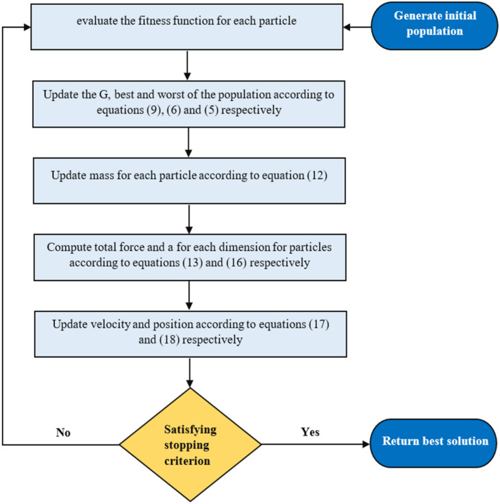
Step eight: Repeat steps two to seven until the stop criteria are reached; these eight steps are illustrated by a flowchart shown in Fig. 2.
Fig. 2.
GSA flowchart.
2.2. Convolutional neural networks
In this section, the main structure of any CNN architecture will be illustrated. Additionally, the transfer learning method and how to apply this method using a pre-trained CNN architecture will be explained.
Network Structure: CNN architectures consist of two bases, namely convolutional base and classifier base.
The convolutional base includes three significant types of layers are: convolutional layers [31], activation layers [32], and pooling layers [33]. These types of layers are used to discover the basic features of input images, which are called feature maps. A feature map is getting by performing convolution processes to the input image or prior features using a linear filter, merging a bias term. Then passing this feature map through a non-linear activation function such as Sigmoid [34] and Rectified Linear Unit (RELU) [35]. In contrast, the classifier base includes the dense layers combined with the activation layers to convert the feature maps to one dimension vectors to expedite the classification task using many neurons. Usually, one or more dropout layers [36] are added to the classifier base to minimize the overfitting that may encounter CNN architectures and improve their generalization. Adding any dropout layer to the classifier base introduces a new hyperparameter called dropout rate. This hyperparameter determines the probability at which outputs of the layer are removed, or reciprocally, the probability at which outputs of the layer are kept. Typically, the dropout rate is set in the range from 0.1 to 0.9 [37].
Transfer Learning: One of the famous and very influential techniques for dealing with small datasets is using a pre-trained network. A pre-trained network is a network that was trained on a vast dataset, usually in the task of categorizing images, and then its architecture and weights were preserved. If this initial dataset is big enough and general enough, the set of features that the pre-trained network has learned can be useful as a general visual model. Therefore, these features can help several different computer vision tasks, even if the new tasks may contain fully different categories from the initial task [38], [39]. For example, networks that have been trained on the ImageNet database, such as DenseNet121 [40], can reset to something as remote as exploring medical image features. Transfer learning from a pre-trained network can be applied in two ways, namely feature extraction and fine-tuning. The Feature extraction involves taking the convolutional base of a pre-trained network to extract the new dataset features and then training a new classifier on top of these outputs. The fine-tuning is complementary to the feature extraction method, where it involves unfreezing the last layers of the frozen convolutional base utilized for the feature extraction. The unfrozen layers are then retrained in combination with the new classifier previously learned in the feature extraction method. The fine-tuning method aims to adjust the pre-trained model’s most abstract features to make them more relevant to the new task. The steps for using these ways can be explained as follows [41]:
-
-
A pre-trained network is taken, and its classifier base is removed.
-
-
The convolutional base of the pre-trained model is frozen.
-
-
A new classifier is added and trained on top of the convolutional base of the pre-trained network.
-
-
Unfreeze some layers of the convolutional base of the pre-trained network.
-
-
Finally, both these unfrozen layers and the new classifier are jointly trained.
3. Binary COVID-19 dataset description
The binary COVID-19 dataset used in this paper is a combination of two datasets. The first dataset is the COVID19 Chest X-ray dataset made available by Dr. Joseph Paul Cohen of the University of Montreal [42]. The COVID19 Chest X-ray dataset consists of 150 chest X-ray and CT images as of the time of writing this paper, 121 images of this dataset represent cases infected with the COVID-19. While 11 images represent cases infected with SARS, and four images represent cases infected with acute respiratory distress syndrome (ARDS). This dataset also contains five pneumocystis cases and six cases of streptococcus, as shown in Table 1.
Table 1.
Number of cases of COVID-19, SARS, ARDS, Pneumocystis and Streptococcus, number of cases diagnosed with X-rays, and CT scans in each cause of pneumonia, and the total number of cases in the COVID19 Chest X-ray dataset.
| The cause of pneumonia | Total number of samples | Number of cases diagnosed with X-ray images | Number of cases diagnosed with CT scans |
|---|---|---|---|
| COVID-19 | 121 | 99 | 22 |
| SARS | 11 | 11 | – |
| ARDS | 4 | 4 | – |
| Pneumocystis | 6 | 6 | – |
| Streptococcus | 2 | 2 | – |
| Undefined | 6 | 6 | – |
| Total | 150 | 128 | 22 |
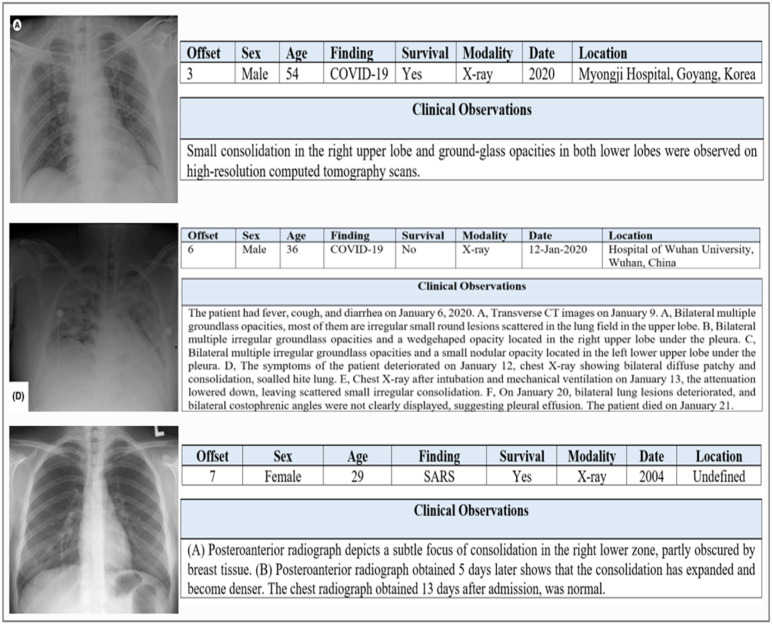
The COVID19 Chest X-ray dataset contains many metadata for each image. The most important of which are: offset, sex, age, finding, survival, modality, date, location, and clinical observations about the radiograph in particular, not just the patient. The offset is the number of days since the onset of symptoms or hospitalization; the offset values ranged from 0 to 32. The ages of the patients enrolled in this dataset ranged from 12 to 87. While the finding field explains the cause of pneumonia, and the surviving field clarifies whether the patient is still alive or not. The modality defines how the diagnosis was made, either X-ray or CT scan. Fig. 3 shows some samples of the COVID19 Chest X-ray dataset and metadata for each sample.
Fig. 3.
Some images of the COVID19 Chest X-ray dataset, next to each image is its metadata.
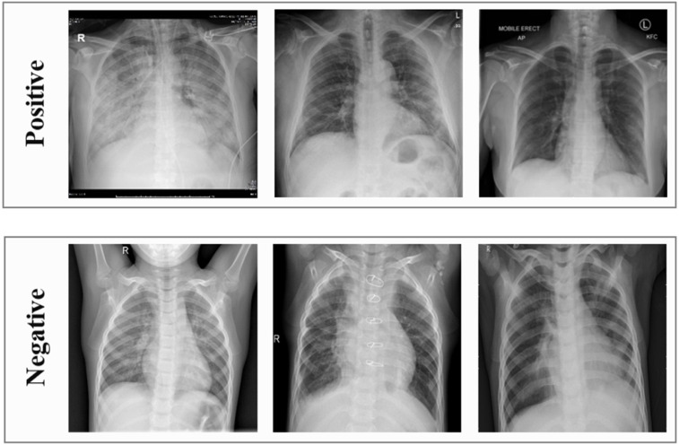
The second dataset is the Kaggle Chest X-ray dataset made available for a Data Science competition [43]. This dataset consists of 5811 X-ray images, 1538 images represent normal cases, and 4273 images represent pneumonia cases. The binary COVID-19 dataset was built to distinguish COVID-19 cases from those suffering from other diseases and healthy cases using only X-ray images. The cases that were diagnosed using CT scans were excluded. The used dataset consists of two categories: positive and negative, as shown in Table 2. The positive category contains 99 X-ray images representing cases infected with the COVID-19, taken from the COVID19 Chest X-ray dataset. The negative category contains 207 X-ray images, 104 images in this category represent healthy cases, and 80 images represent pneumonia cases, taken from the Kaggle Chest X-ray dataset. The other 23 images in the negative category represent cases affected by SARS, ARDS, pneumocystis, or streptococcus, taken from the COVID19 Chest X-ray dataset. Some images of each category of the binary COVID-19 dataset are shown in Fig. 4.
Table 2.
Details of samples included in each category of the binary COVID-19 dataset in terms of sample type, number of samples, and sample source. For each category, the total number of samples is reported.
| Category | Sample type | Number of samples | Sample source | Total number of samples in the category |
|---|---|---|---|---|
| Positive | COVID-19 | 99 | COVID19 Chest X-ray dataset | 99 |
| Negative | Healthy | 104 | Kaggle Chest X-ray dataset | 207 |
| Pneumonia | 80 | Kaggle Chest X-ray dataset | ||
| SARS | 11 | COVID19 Chest X-ray dataset | ||
| ARDS | 4 | COVID19 Chest X-ray dataset | ||
| Pneumocystis | 6 | COVID19 Chest X-ray dataset | ||
| Streptococcus | 2 | COVID19 Chest X-ray dataset | ||
Fig. 4.
Representative images of the positive and negative categories of the binary COVID-19 dataset.
4. The proposed GSA-DenseNet121-COVID-19 approach
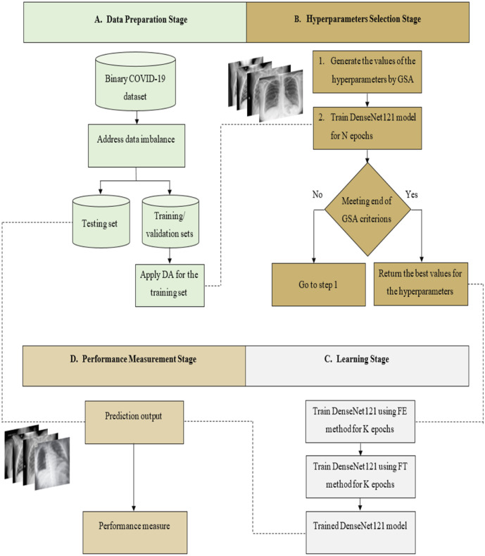
The proposed approach GSA-DenseNet121-COVID-19, relies on the transfer learning from a pre-trained CNN architecture. The pre-trained architecture utilized in the proposed approach is DenseNet121. For this architecture’s best performance, its hyperparameters have been optimized using the GSA. After determining the optimal values for these hyperparameters, DenseNet121 was trained using transfer learning techniques. Once this training is completed, it is evaluated using a separate test set. In other words, the training and validation sets were used to determine the optimal values for the hyperparameters of the DenseNet121 and trained it. Whereas the fully trained DenseNet121 is then evaluated using the test set. The proposed approach consists of four main stages, as shown in Fig. 5. The first stage is the data preparation, the second stage is the hyperparameters selection, the third stage is the learning, and the performance measurement is the fourth stage. Each stage will be explained in detail in the following sections.
Fig. 5.
The structural form of the proposed approach GSA-DenseNet121-COVID-19 for the binary COVID-19 dataset, DA=Data Augmentation, FE=Feature Extraction, FT=Fine Tuning.
4.1. Data preparation stage
As explained in the data description section, the positive category of the binary COVID-19 dataset contains 99 samples, while the negative category includes 207 samples, which means that this dataset is not balanced. In most cases, not all ML algorithms can handle this type of dataset well. Because most of the information available in this type of dataset belongs to the dominant category, making any ML algorithm learn to categorize the dominant class and not categorize the other minor category. Therefore, samples in the positive category have been increased by randomly copying some images after cutting each image. So that random copying does not cause the used CNN architecture to overfit the dataset. After that, the dataset became balanced, with each category containing 207 images.
The balanced binary COVID-19 dataset was divided into three sets: training set, validation set, and testing. The training set contains 70% of the dataset; that is, it has about 146 images in each category. While each of the validation and the test set contains 15% of the dataset samples; that is, each set includes 31 images in each category. Various data augmentation techniques [44] have been applied to increase the number of training samples to reduce overfitting and improve generalization. The data augmentation techniques used are brightness, rotation, width shift, height shift, shearing, zooming, vertical flip, and horizontal flip. Also, featurewise centering, featurewise standard deviation normalization and fill mode. Before the images were supplied to other stages, they were resized to a 180 x 180.
4.2. Hyperparameters selection stage
As previously reviewed in Section 2.2, the transfer learning method takes the same structure of the pre-trained network after making minor changes. The most crucial change is to replace the classifier with a new one, which requires changing the values of some hyperparameters or adding new ones. Examples of the hyperparameters that require modification are the batch size, the learning rat’s value, and the number of neurons in the dense layer. The hyperparameter that may add is the rate of the dropout layer. In the proposed GSA-DenseNet121-COVID-19, three hyperparameters have been optimized, namely the batch size, the rate of the newly added dropout layer, and the number of the neurons of the first dense layer. Therefore, the search space is three-dimensional, and each point in the space represents a mixture of these three hyperparameters.
4.3. Learning stage
The feature extraction and fine-tuning techniques are utilized to prepare the DenseNet121 architecture to learn from the binary COVID-19 dataset. In the feature extraction, the convolutional base is kept unchanged, Whereas, the original classifier base is replaced by a new one that fits the binary COVID-19 dataset. The new classifier consists of four stacked layers: a flatten layer, and two dense layers separated by a new dropout layer. GSA determines the number of neurons in the first dense layer that uses RELU as an activation function and the dropout layer rate. The second dense layer has one neuron with a sigmoid function. After training the new classifier for some epochs, the fine-tuning is configured by retraining the last two blocks of the convolutional base of the DenseNet121 with the newly added classifier simultaneously.
4.4. Performance measurement stage
At this phase, the proposed approach is evaluated. Six measures are utilized to evaluate the proposed approach, namely accuracy, precision, recall, F1 score, and confusion matrix. Accuracy is among the foremost remarkably used measures for measuring the performance of classification models. It is outlined as a proportion between correctly classified samples to the overall number of samples as shown in Eq. (19). The error rate is the complement of the accuracy; it represents the samples that are misclassified by the model and calculated as Eq. (20) [45].
| (19) |
| (20) |
Where P= the number of the positive samples, and N= the numbers of the negative samples.
Precision as shown in Eq. (21), it is the number of true positives divided by the number of true positives and false positives. In other words, it is the number of positive predictions divided by the total number of positive category values predicted. Precision can be considered a measure of the rigor of a classifier. A low precision can also indicate a large number of false positives [46].
| (21) |
Recall, which also termed as sensitivity is the number of true positives divided by the number of true positives and the number of false negatives as shown in Eq. (22). In other words, it is the number of positive predictions divided by the number of positive class values in the test set. Recall can be considered a measure of how complete a classifier is. A low Recall indicates many false negatives [46].
| (22) |
F1 score, which is also termed as F score, is a function of precision and recall and calculated as Eq. (23). It is used to seek a balance between precision and recall [46].
| (23) |
Confusion Matrix is a synopsis of the prediction results regarding the classification problem. The confusion matrix gives insight into not only the mistakes committed by the classifier but, more importantly, the types of errors that are made [47].
5. Experiment results
This section presents and analyzes the results obtained through the proposed approach described in detail in Section 4. All the proposed approach procedures have been executed on Google Colaboratory [48] and implemented using Python with Keras [49]. Keras is a high-level neural network API, written in Python and capable of running on top of TensorFlow, CNTK, or Theano. It was developed for rapid use and the ability to conduct several experiments and get results as quickly as possible and the lowest delay, which helps to conduct adequate research. The results are divided into five sections to display clearly.
5.1. Conducting the data augmentation techniques
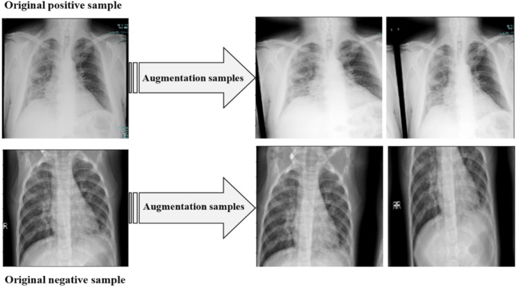
The Keras ImageDataGenerator was utilized to implement augmentation techniques to increase the number of images of the binary COVID-19 dataset’s training set. The data augmentation techniques used and the range used for each technique are listed in Table 3. Fig. 6 illustrates some of the images obtained by applying augmentation techniques to one image from each category.
Table 3.
The augmentation techniques and the range of each technique.
| Augmentation technique | Range |
|---|---|
| Shearing | 0.2 |
| Zooming | 0.3 |
| Width shift | 0.4 |
| Height shift | 0.4 |
| Rotation | 15 |
| Brightness | [0.5, 1.5] |
| Featurewise center | True |
| Featurewise standard deviation normalization | True |
| Fill mode | Reflect |
| Vertical flip | True |
| Horizontal flip | True |
Fig. 6.
Some samples generated from applying various augmentation techniques.
5.2. Setting up the GSA for the hyperparameters selection stage
The search space for hyperparameters whose values are to be set by the GSA was bounded as follows. The searching range of batch size was bounded by [1,64], and the searching space of the dropout rate was bounded by [0.1,0.9]. While the searching space of the number of neurons is bounded by [5,500], as listed in Table 4.
Table 4.
Preparation of the required parameter values for GSA in conjunction with DensNet121.
| Parameter | Value |
|---|---|
| Maximum number of iterations | 15 |
| Population size | 30 |
| Dimension | 3 |
| Batch size bounds | [1,64] |
| Dropout rate bounds | [0.1,0.9] |
| Number of neurons bounds | [50,500] |
| Maximum number of DenseNet121 training epochs | 10 |
The GSA parameters’ values were randomly specified, where the maximum number of iteration and population size set to 15 and 30, respectively, as listed in Table 4. The number of DenseNet121 training epochs was chosen by experimenting with more than one value. The experiment concluded that when using a number of epochs over ten, the training process for each of the GSA takes exponential time. While when using less than ten epochs, the results of the DenseNet121 were not sufficiently accurate. Therefore, the number of epochs used to train the DenseNet121 was set to ten epochs. The goal of using the GSA is to reduce the loss rate of the validation set as much as possible. The proposed GSA solutions’ suitability is evaluated based on the achieved loss rate of the validation set using these proposed solutions after ten network training periods.
After completing the approximately 11-hour GSA training, the optimum values for the batch size, dropout rate, and number of neurons of the first dense layer were determined. Table 5 shows the optimal values for the hyperparameters selected by GSA, where the batch size, dropout and the number of neurons are 8, 0.1, 110 respectively.
Table 5.
Optimal values for the hyperparameters that were determined by GSA.
| Hyperparameters | Optimal values |
|---|---|
| Batch size | 8 |
| Dropout rate | 0.1 |
| Number of neurons of the first dense layer | 110 |
5.3. Learning the DenseNet121 using the optimized hyperparameters
At this stage, the DenseNet121 was trained using the optimal values for the hyperparameters chosen by GSA. DenseNet121 architecture was trained on the training set and evaluated on the validation set for K number of epochs. To determine the value of K, several experiments were conducted, and it was found that the DenseNet121 achieved the best results on the validation set around the 30th epoch within the feature extraction method. While about the 40th epoch within the fine-tuning method and that no improvement was observed after that. Thus, the value of K was marked to 30 within the feature extraction and 40 within the fine-tuning. To minimize the overfitting, the process of the training was forced to finish before repetition K if no improvement was perceived for seven iterations, this control was made using early stopping [50]. As the COVID-19 dataset used is a binary-class classification problem, the DenseNet121 is compiled with the binary cross-entropy [51]. The Adam optimizer algorithm [52] was used with a constant learning rate =2e-5 within the feature extraction method. Within the fine-tuning method, a step decay schedule [53] was utilized, where the initial learning rate , and the value of the learning rate drops by 0.5 every 10 training epochs. The use of a low learning rate in the fine-tuning method is due to the fact that the number of changes that will occur in this method should be very small. So that the features learned from the feature extraction method are not lost.
5.4. Measuring the performance of GSA-DenseNet121-COVID-19
This section presents the results of the performance evaluation of the DenseNet121 architecture using hyperparameters values specified by the GSA. The performance of the proposed approach GSA-DenseNet121-COVID-19 was evaluated using accuracy, loss rate, precision, recall, and F1 score. The proposed approach achieved 98.38% accuracy in the test set, the average precision, recall, and f1 score were 98.5%, 98.5%, and 98%, respectively. The macro average and weighted average for the precision, recall, and F score was equal as the values for both were 98%, as listed in Table 6.
Table 6.
The performance of the proposed approach GSA-DenseNet121-COVID-19 and the overall performance is calculated using macro and weighted average.
| Categories | Precision | Recall | F1 score |
|---|---|---|---|
| Negative | 97% | 100% | 98% |
| Positive | 100% | 97% | 98% |
| Average | 98.5% | 98.5% | 98% |
| Macro Average | 98% | 98% | 98% |
| Weighted Average | 98% | 98% | 98% |
To find out the number of samples incorrectly classified by the proposed approach
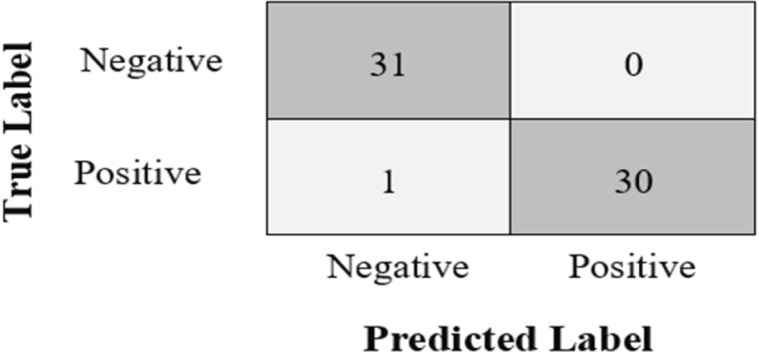
GSA-DenseNet121-COVID-19. As well as the number of samples that it was able to classify correctly, the confusion matrix was used as shown in Fig. 7. The dark-colored shaded cells of the confusion matrix represent samples that were correctly categorized in each category. Whereas, the light-colored shaded cells of the confusion matrix represent incorrectly categorized samples in each category.
Fig. 7.
The confusion matrix obtained from the proposed approach GSA-DenseNet121-COVID-19.
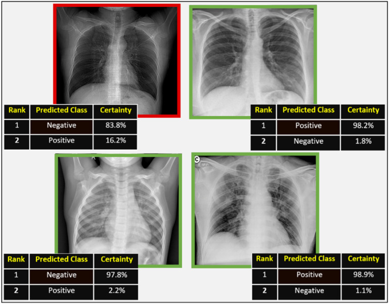
As shown in the confusion matrix in Fig. 7, the proposed approach GSA-DenseNet121-COVID-19 erroneously classified only one sample from the test group, while it succeeded in classifying all other samples. Fig. 8 shows the results of the proposed approach for four images. The images surrounded by a green rectangle represent the images that the proposed approach correctly classified. While the image surrounded by the red rectangle represents the only sample that the proposed approach has incorrectly classified. The image in the red rectangle is an image that belongs to the positive category. However, the proposed approach classified this image as belonging to the negative category with a certainty of 83.8% as a first decision and to a positive category with a certainty of 16.2% as a second decision.
Fig. 8.
Illustrative examples of some correctly labeled samples (enclosed in a green rectangle) and the incorrectly labeled sample (enclosed in a red rectangle) from the test set.
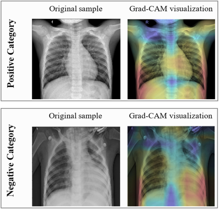
To know whether the proposed GSA-DenseNet121-COVID-19 is aware of X-rays as radiologists do, or whether it is learning unhelpful features to make predictions. The gradient weighted class activation mapping (Grad-CAM) [54] was used. As shown in Fig. 9, the Grad-CAM visualization of a positive sample and a negative sample, prove the effectiveness of the proposed approach in determining the important features relevant to each category.
Fig. 9.
The Grad-CAM visualization of a positive sample and a negative sample.
5.5. Comparison with other methods and related work
To ensure the effectiveness of the GSA in determining optimum values for the hyperparameters of the DenseNet121 architecture that can achieve the highest level of accuracy. It has been compared with the SSD algorithm [55] that has been proven effective in determining optimal values for the hyperparameters of the CNN architecture used to detect the nanoscience scanning electron microscope images [25]. For a fair comparison between GSA and SSD algorithm. The values of the SSD algorithm parameters have been set with the same values that have been set for the GSA parameters, as shown in Table 4. After the SSD algorithm has completed the training process, the batch size value was set to 6, while the number of neurons and the dropout rate were set to 220 and 0.71, respectively. The comparative results showed that the GSA is more suitable for pairing with the DenseNet121 to classify the binary COVID-19 dataset. Where the GSA was able to choose better values for the hyperparameters of DenseNet121 architecture, which in turn made this architecture achieve a higher accuracy ratio. Where the approach SSD-DenseNet121 achieved an accuracy rate of 94% on the test set. As well as the macro average for the precision, recall, F1 score of the SSD-DenseNet121 were equal as the values for both were 94%, as listed in Table 7.
Table 7.
Comparison of the proposed GSA-DenseNet121-COVID-19 performance with the performance of the SSD-GSA approach and Inception-v3. MA-Precisionmacro average of precision, MA-Recall macro average of recall, and MA-F score macro average of F-score.
| Comparison items | Proposed approach | SSD-DenseNet121 | Inception-v3 |
|---|---|---|---|
| Batch size | 8 | 6 | 10 |
| Dropout rate | 0.1 | 0.71 | 0.5 |
| Number of neurons | 110 | 220 | 150 |
| Accuracy | 98.38% | 94% | 95% |
| MA-Precision | 98% | 94% | 96% |
| MA-Recall | 98% | 94% | 95% |
| MA-F Score | 98% | 94% | 95% |
To ensure the performance of the proposed approach GSA-DenseNet121-COVID-19 as a whole. It was compared with the Inception-v3 architecture based on the manual search. The manual search indicates that the values of the Inception-v3 hyperparameters were randomly chosen. Where the values of batch size, dropout rate, and the number of neurons were set manually to 16, 0.5, 250, respectively. The results of this comparison showed that the proposed GSA-DenseNet121-COVID-19 was superior to the Inception-v3 architecture based on the manual search. Where, the accuracy of the Inception-v3 architecture is 95%, while the macro average precision, recall, and F1 score of this architecture are 95%, 96%, 95%, 95%, respectively, as shown in Table 7.
The proposed GSA-DenseNet121-COVID-19 performance was also compared with other published approaches that were introduced for the same purpose of diagnosing COVID-19 using X-ray images. The other approaches included in [14], [15], [16], [17], [19] were selected for comparison, as they relied on CNN architectures and were trained on a variety of data samples. The proposed approach has been compared to other approaches in terms of the number and variety of samples used, accuracy, precision, recall, and f score, as shown in Table 8. In [14], many of the CNN architectures were evaluated to classify two datasets. However, the best performance was for the MobileNet architecture on the second dataset containing 224 samples of COVID-19, 504 healthy samples, and 714 samples of pneumonia. The MobileNet obtained an accuracy, precision, and recall rate of 96.78%, 96.46%, and 98.66%, respectively, in the second dataset classification when it was treated as a binary classification problem, as shown in the second row of Table 8. In [15], the proposed DarkCovidNet was able to be more accurate by classifying the two categories more than classifying the three categories, as shown in rows 3 and 4 of Table 8. Whereas in [16], after the CNN-SA approach was trained in healthy and COVID-19 cases only, it was able to achieve a rate of 96% for both accuracy, precision, recall, and f score. The CoroNet proposed in [17] has performed better in the binary classification that includes only healthy and COVID-19 cases, than the multi-category classification that includes various types of samples, as shown in rows 5, 6, and 7 of Table 8. While the Deep Bayes-SqueezeNet approach [19], having been trained on a relatively large number of samples, was able to achieve 97% for both accuracy, precision, recall, and f score, as shown in the eighth row of Table 8.
Table 8.
A comparison between the results of the proposed approach and the best results achieved by the other proposed approaches listed in [14], [15], [16], [17], [19].
| Approach | Number of original samples | Number of classes | Accuracy | Average precision |
Average Recall |
Average F score |
|---|---|---|---|---|---|---|
| MobileNet [14] | 224 COVID-19 504 Healthy 714 Pneumonia (400 bacterial + 314 viral) |
2 classes | 96.78% | 96.46% | 98.66% | – |
| DarkCovidNet [15] | 125 COVID-19 500 No- Findings |
2 classes | 98.08%. | 98.03% | 95.13% | 96.51% |
| DarkCovidNet [15] | 125 COVID-19 500 No- Findings 500 Pneumonia |
3 classes | 87.02% | 89.96% | 85.35% | 87.37% |
| CNN-SA [16] | 403 COVID-19 721 Normal |
2 classes | 95% | 95% | 95% | 95% |
| CoroNet [17] | 284 COVID-19 310 Normal 330 Pneumonia Bacterial 327 Pneumonia Viral |
4 classes | 89.6% | 90% | 89.92% | 89.8% |
| CoroNet [17] | 284 COVID-19 310 Normal 657 Pneumonia (330 bacterial + 327 viral) |
3 classes | 95% | 95% | 96.9% | 95.6% |
| CoroNet [17] | 284 COVID-19 310 Normal |
2 classes | 99% | 98.3% | 99.3% | 98.5% |
| Deep Bayes-SqueezeNet [19] | 76 COVID-19 4290 Pneumonia (bacterial + viral) 1583 Normal |
3 classes | 98.3% | 98.3% | 98.3% | 98.3% |
|
Proposed GSA-DenseNet121-COVID-19 |
99 COVID-19 11 SARS 4 ARDS 6 Pneumocystis 2 Streptococcus 104 Healthy 80 pneumonia |
2 classes | 98.38% | 98.5% | 98.5% | 98% |
Table 8 shows that although the proposed GSA-DenseNet121-COVID-19 has been trained in a smaller and more diverse number of samples than its counterparts. The proposed GSA-DenseNet121-COVID-19 managed to outperform both DarkCovidNet and CNN-SA. Likewise, the results of GSA-DenseNet121-COVID-19 outperformed the results of MobileNet in terms of accuracy and precision but were slightly smaller in the recall. The proposed GSA-DenseNet121-COVID-19 is very competitive with the Deep Bayes-SqueezeNet. Since the results of GSA-DenseNet121-COVID-19 are better than the results of Deep Bayes-SqueezeNet in terms of precision and recall, they are approximately equal in accuracy and slightly less in result f score. The DenseNet121-COVID-19 was superior to the CoroNet when the latter was trained on a variety of samples, just as the DenseNet121-COVID-19 was trained.
6. Conclusions and future work
This paper proposes an approach called GSA-DenseNet121-COVID-19 that can be used to diagnose COVID-19 cases through chest X-ray images. The proposed GSA-DenseNet121-COVID-19 consists of four main stages are (1) data preparation stage, (2) the hyperparameters selection stage, (3) the learning stage, (4) the performance measurement stage. In the first stage, the binary COVID-19 dataset was handled from the imbalance and then divided into three sets, namely training set, validation set, and test set. After increasing the number of samples of the training set in the first stage using different data augmentation techniques, they were used in the second stage with the validation set. In the second stage, GSA is used to optimize some of the hyperparameters in the CNN architecture used which is called DenseNet121. In the third stage, DenseNet121 was completely trained using the values of the hyperparameters that were identified in the previous stage which in turn helped this architecture to diagnose 98.38% of the test set in the fourth stage. The proposed approach was compared to more than one approach, and the results of the comparison showed the effectiveness of the proposed approach in diagnosing the COVID-19. In future work, the number of samples used to train the proposed approach can be increased to improve its performance in the diagnosis of COVID-19. In addition, the number of other diseases causing pneumonia may be increased and the proposed approach can be used to distinguish them from the COVID-19.
Declaration of Competing Interest
The authors declare that they have no known competing financial interests or personal relationships that could have appeared to influence the work reported in this paper.
References
- 1.Vivaldo G. The emergence of SARS, MERS and novel SARS-2 coronaviruses in the 21st century. Arch. Virol. 2020;165(7):1517–1526. doi: 10.1007/s00705-020-04628-0. [DOI] [PMC free article] [PubMed] [Google Scholar]
- 2.Fouchier R.A. Aetiology: Koch’s postulates fulfilled for SARS virus. Nature. 2003;423(6937) doi: 10.1038/423240a. 240–240. [DOI] [PMC free article] [PubMed] [Google Scholar]
- 3.Zaki A.M. Isolation of a novel coronavirus from a man with pneumonia in Saudi Arabia. New Engl. J. Med. 2012;367(19):1814–1820. doi: 10.1056/NEJMoa1211721. [DOI] [PubMed] [Google Scholar]
- 4.Centers for Disease Control and Preventio . second ed. U.S. Department of Health and Human Services; Atlanta: 1992. Principles of Epidemiology. [Online]. Available: https://www.cdc.gov/csels/dsepd/ss1978/lesson1/section9.html. [Google Scholar]
- 5.Broughton J.P. CRISPR–Cas12-based detection of SARS-CoV-2. Nature Biotechnol. 2020;38:870–874. doi: 10.1038/s41587-020-0513-4. [DOI] [PMC free article] [PubMed] [Google Scholar]
- 6.Alireza T. Real-time RT-PCR in COVID-19 detection: issues affecting the results. Expert Rev. Mol. Diagnost. 2020;20(5):1–2. doi: 10.1080/14737159.2020.1757437. [DOI] [PMC free article] [PubMed] [Google Scholar]
- 7.Talo M., Baloglu U.B., Yıldırım Ö., Acharya U.R. Application of deep transfer learning for automated brain abnormality classification using MR images. Cogn. Syst. Res. 2019;54(14):176–188. [Google Scholar]
- 8.Ismael S.A.A., Mohammed A., Hefny H. An enhanced deep learning approach for brain cancer MRI images classification using residual networks. Artif. Intell. Med. 2020;102 doi: 10.1016/j.artmed.2019.101779. [DOI] [PubMed] [Google Scholar]
- 9.Khalifa N.E.M., Taha M.H.N., Ali D.E., Slowik A., Hassanien A.E. Artificial intelligence technique for gene expression by tumor RNA-seq data: A novel optimized deep learning approach. IEEE Access. 2020;8:22874–22883. [Google Scholar]
- 10.Ho C., Jean N., Hogan C.A., Blackmon L., Jeffrey S.S., Holodniy M., Banaei N., Saleh A.A.E., Ermon S., Dionne J. Rapid identification of pathogenic bacteria using Raman spectroscopy and deep learning. Nature Commun. 2019;10(1):1–8. doi: 10.1038/s41467-019-12898-9. [DOI] [PMC free article] [PubMed] [Google Scholar]
- 11.Haque I.R.I., Neubert J. Deep learning approaches to biomedical image segmentation. Inf. Med. Unlocked. 2020;18 [Google Scholar]
- 12.LeCun Y., Bengio Y., Hinton G. Deep learning. Nature. 2015;521(7553):436–444. doi: 10.1038/nature14539. [DOI] [PubMed] [Google Scholar]
- 13.Erickson B.J., Korfiatis P., Kline T.L., Akkus Z., Philbrick K., Weston A.D. Deep learning in radiology: Does one size fit all? J. Am. Coll. Radiol. 2018;15(3):521–526. doi: 10.1016/j.jacr.2017.12.027. [DOI] [PMC free article] [PubMed] [Google Scholar]
- 14.Apostolopoulos I.D., Mpesiana T.A. Covid-19: automatic detection from X-ray images utilizing transfer learning with convolutional neural networks. Phys. Eng. Sci. Med. 2020;43(2):635–640. doi: 10.1007/s13246-020-00865-4. [DOI] [PMC free article] [PubMed] [Google Scholar]
- 15.Ozturk T., Talo M., Yildirim E.A., Baloglu U.B., Yildirim O., Acharya U.R. Automated detection of COVID-19 cases using deep neural networks with X-ray images. Comput. Biol. Med. 2020;121 doi: 10.1016/j.compbiomed.2020.103792. [DOI] [PMC free article] [PubMed] [Google Scholar]
- 16.Waheed A., Goyal M., Gupta D., Khanna A., Al-Turjman F., Pinheiro P.R. CovidGAN: Data augmentation using auxiliary classifier GAN for improved Covid-19 detection. IEEE Access. 2020;8:91916–91923. doi: 10.1109/ACCESS.2020.2994762. [DOI] [PMC free article] [PubMed] [Google Scholar]
- 17.Khan A.I., Shah J.L., Bhatc M.M. CoroNet: A deep neural network for detection and diagnosis of COVID-19 from chest x-ray images. Comput. Methods Programs Biomed. 2020;196 doi: 10.1016/j.cmpb.2020.105581. [DOI] [PMC free article] [PubMed] [Google Scholar]
- 18.Ucara F., Korkmazb D. COVIDiagnosis-Net: Deep Bayes-SqueezeNet based diagnosis of the coronavirus disease 2019 (COVID-19) from X-ray images. Med. Hypotheses. 2020;140 doi: 10.1016/j.mehy.2020.109761. [DOI] [PMC free article] [PubMed] [Google Scholar]
- 19.Koutsoukas A., Monaghan K.J., Li X., Huan Jun. Deep-learning: investigating deep neural networks hyper-parameters and comparison of performance to shallow methods for modeling bioactivity data. J. Cheminformat. 2017;9(42) doi: 10.1186/s13321-017-0226-y. [DOI] [PMC free article] [PubMed] [Google Scholar]
- 20.Albelwi S., Mahmood A. A framework for designing the architectures of deep convolutional neural networks. Entropy. 2017;19(6):242. [Google Scholar]
- 21.Bergstra J., Bengio Y. Random search for hyper-parameter optimization. J. Mach. Learn. Res. 2012;13(1):281–305. [Google Scholar]
- 22.Young S.R., Rose D.C., Karnowski T.P., Lim S., Patton R.M. Proceedings of the Workshop on Machine Learning in High-Performance Computing Environments (MLHPC 2015) ACM; Austin, Texas: 2015. Optimizing deep learning hyper-parameters through an evolutionary algorithm; pp. 1–5. [Google Scholar]
- 23.Yoo Y. Hyperparameter optimization of deep neural network using univariate dynamic encoding algorithm for searches. Knowl.-Based Syst. 2019;178:74–83. [Google Scholar]
- 24.Darwish A., Ezzat D., Hassanien A.E. An optimized model based on convolutional neural networks and orthogonal learning particle swarm optimization algorithm for plant diseases diagnosis. Swarm Evol. Comput. 2020;52 [Google Scholar]
- 25.Ezzat D., Taha M.H.N., Hassanien A.E. Proceedings of the International Conference on Advanced Intelligent Systems and Informatics 2019 (AISI 2019) Springer; Cairo, Egypt: 2020. An optimized deep convolutional neural network to identify nanoscience scanning electron microscope images using social ski driver algorithm; pp. 492–501. [Google Scholar]
- 26.Rashedi E., Nezamabadi-pour H., Saryazdi S. GSA: A gravitational search algorithm. Inform. Sci. 2009;179(13):232–2248. [Google Scholar]
- 27.Holliday D., Resnick R., Walker J. John Wiley and Sons; 2013. Fundamentals of Physics. [Google Scholar]
- 28.Schutz B.F. Cambridge University Press; 2003. Gravity from the Ground Up: An Introductory Guide to Gravity and General Relativity. [Google Scholar]
- 29.Mansouri R., Nasseri F., Khorrami M. Effective time variation of G in a model universe with variable space dimension. Phys. Lett. 1999;259(3–4):194–200. [Google Scholar]
- 30.Yuana X., Ji B., Zhang Shuangquan., Tiana H., Houa Y. A new approach for unit commitment problem via binary gravitational search algorithm. Appl. Soft Comput. 2014;22:249–260. [Google Scholar]
- 31.Rawat W., Wang Z. Deep convolutional neural networks for image classification: A comprehensive review. Neural Comput. 2017;29(9):2352–2449. doi: 10.1162/NECO_a_00990. [DOI] [PubMed] [Google Scholar]
- 32.Jang J., Cho H., Kim J., Lee J., Yang S. Deep neural networks with a set of node-wise varying activation functions. Neural Netw. 2020;126:118–131. doi: 10.1016/j.neunet.2020.03.004. [DOI] [PubMed] [Google Scholar]
- 33.Suárez-Paniagua V., Segura-Bedmar I. Evaluation of pooling operations in convolutional architectures for drug-drug interaction extraction. BMC Bioinformatics. 2018;19(8):39–47. doi: 10.1186/s12859-018-2195-1. [DOI] [PMC free article] [PubMed] [Google Scholar]
- 34.Wang Y., Li Y., Song Y., Rong X. The influence of the activation function in a convolution neural network model of facial expression recognition. Appl. Sci. 2020;10(5):1897. [Google Scholar]
- 35.X. Glorot, A. Bordes, Y. Bengio, Deep sparse rectifier neural networks, in: Proceedings of the 14th International Conference on Artificial Intelligence and Statistics, Fort Lauderdale, FL, USA, 2011, pp. 315–323.
- 36.Srivastava N., Hinton G., Krizhevs.ky A., Sutskever I., Salakhutdinov R. Dropout: A simple way to prevent neural networks from overfitting. J. Mach. Learn. Res. 2014;15(1):1929–1958. [Google Scholar]
- 37.Goodfellow I., Bengio Y., Courville A. MIT Press; Cambridge: 2016. Deep Learning, vol. 1. [Google Scholar]
- 38.Lumini A., Nanni L. Deep learning and transfer learning features for plankton classification. Ecol. Inform. 2019;51:33–43. [Google Scholar]
- 39.Barbedo J.G.A. Impact of dataset size and variety on the effectiveness of deep learning and transfer learning for plant disease classification. Comput. Electron. Agric. 2018;153:46–53. [Google Scholar]
- 40.G. Huang, Z. Liu, L. Van Der Maaten, K.Q. Weinberger, Densely Connected Convolutional Networks, in: Proceedings of the IEEE conference on computer vision and pattern recognition, 2017, pp. 2261–2269.
- 41.Yamashita R., Nishio M., Do R.K.G., Togashi K. Convolutional neural networks: an overview and application in radiology. Insights Imaging. 2018;9(4):611–629. doi: 10.1007/s13244-018-0639-9. [DOI] [PMC free article] [PubMed] [Google Scholar]
- 42.2020. COVID-19 image data collection. [Online]. Available: https://github.com/ieee8023/covid-chestxray-dataset. (Accessed 25 March 25 2020) [Google Scholar]
- 43.2020. Chest X-ray images (Pneumonia) [Online]. Available: https://www.kaggle.com/paultimothymooney/chest-xray-pneumonia. (Accessed 25 March 25 2020) [Google Scholar]
- 44.Shorten C., Khoshgoftaar T.M. A survey on image data augmentation for deep learning. J. Big Data. 2019;6(1):60. doi: 10.1186/s40537-021-00492-0. [DOI] [PMC free article] [PubMed] [Google Scholar]
- 45.Tharwat A. Classification assessment methods. Appl. Comput. Inf. 2018 [Google Scholar]
- 46.Goutte C., Gaussier E. Proceedings of European Conference on Information Retrieval. Springer; Berlin, Heidelberg: 2005. A probabilistic interpretation of precision, recall and f-score, with implication for evaluation; pp. 345–359. [Google Scholar]
- 47.Ting K.M. Confusion Matrix. Springer; Boston, MA, USA: 2011. p. 209. (Encyclopedia of Machine Learning). [Google Scholar]
- 48.Carneiro T., Medeiros Da NóBrega R.V., Nepomuceno T., Bian G., De Albuquerque V.H.C., Filho P.P.R. Performance analysis of google colaboratory as a tool for accelerating deep learning applications. IEEE Access. 2018;6:61677–61685. [Google Scholar]
- 49.Chollet F. 2015. Keras: Deep learning for humans. [Online]. Available: https://github.com/fchollet/keras. [Google Scholar]
- 50.Prechelt L. Neural Networks: Tricks of the Trade. second ed. 2012. Early stopping - but when? pp. 53–67. [Google Scholar]
- 51.Bosman A.S., Engelbrecht A., Helbig M. Visualising basins of attraction for the cross-entropy and the squared error neural network loss functions. Neurocomputing. 2020;400:113–136. [Google Scholar]
- 52.Kingma D.P., Ba J. 2014. Adam: A method for stochastic optimization. [Online]. Available: arXiv:1412.6980. [Google Scholar]
- 53.A. Senior, G. Heigold, M. Ranzato, K. Yang, An empirical study of learning rates in deep neural networks for speech recognition, in: Proceedings of IEEE International Conference on Acoustics, Speech and Signal Processing, 2013, pp. 6724–6728.
- 54.R.R. Selvaraju, M. Cogswell, A. Das, R. Vedantam, D. Parikh, D. Batra, Grad-CAM: Visual explanations from deep networks via gradient-based localization, in: Proceedings of the IEEE International Conference on Computer Vision, 2017, pp. 618–626.
- 55.Tharwat A., Gabel T. Parameters optimization of support vector machines for imbalanced data using social ski driver algorithm. Neural Comput. Appl. 2019:1–14. [Google Scholar]


