Selective Detection of Water Pollutants Using a Differential Aptamer-Based Graphene Biosensor

Abstract

Graphene field-effect transistor (GFET) sensors are an attractive analytical tool for the detection of water pollutants. Unfortunately, this application has been hindered by the sensitivity of such sensors to nonspecific disturbances caused by variations of environmental conditions. Incorporation of differential designs is a logical choice to address this issue, but this has been difficult for GFET sensors due to the impact of fabrication processes and material properties. This paper presents a differential GFET affinity sensor for the selective detection of water pollutants in the presence of nonspecific disturbances. This differential design allows for minimization of the effects of variations of environmental conditions on the measurement accuracy. In addition, to mitigate the impact of the fabrication process and material property variations, we introduce a compensation scheme for the individual sensing units of the sensor, so that such variations are accounted for in the compensation-based differential sensing method. We test the use of this differential sensor for the selective detection of the water pollutant 17β-estradiol in buffer and tap water. Consistent detection results can be obtained with and without interferences of pH variations, and in tap water where unknown interferences are present. These results demonstrate that the differential graphene affinity sensor is capable of effectively mitigating the effects of nonspecific interferences to enable selective water pollutant detection for water quality monitoring.

1. Introduction

Close monitoring of environmental conditions, such as water pollutants, is critical to human health and food safety. Analytical methods currently used for water pollutant detection, such as gas chromatography/mass spectrometry (GC/MS) and high-performance liquid chromatography (HPLC), are costly, time-consuming and labor-intensive (Janssens et al. 2013; Yildirim et al. 2012). Nanomaterials, emerging as promising candidates, have enabled miniaturized and sensitive sensors to address these challenges for the quantification of pollutants. Graphene, due to its sensitivity and scalability, is of particular interest to enable electronically based environmental sensors (Li et al. 2016; Maity et al. 2017; Wang et al. 2015; Wu et al. 2017). To realize the selective detection of analytes of interest, graphene-based sensors are often functionalized with receptors (e.g., aptamers or antibodies) that possess specific affinity to the target (Lei et al. 2017; Li et al. 2017). Unfortunately, these sensors are also sensitive to nonspecific disturbances in parameters such as pH, ionic strength, and temperature (He et al. 2012). Small fluctuations of these conditions often significantly impact the sensor and produce false signals.

Two methods have been reported to address such nonspecific responses. The first method employs surface blocking, which uses chemicals such as ethanolamine and Tween 20 to block the unmodified surface sites and prevent nonspecific adsorption (Lei et al. 2017; Mao et al. 2017; Xu et al. 2018). However, the sensors are still susceptible to variations in environmental conditions. The second method relies on sample pretreatment. This can remove unwanted interfering molecules and stabilize the sensing conditions (Li et al. 2015; Liang et al. 2017; Tang et al. 2016), but prolongs the time needed to complete the detection process.

Differential measurement approaches, while effectively allowing the minimization or elimination of false signals originating from variations in environmental conditions (Adducci et al. 2016; Fritz et al. 2002; Wipf et al. 2013), have not been explored for graphene sensors in the presence of interferences (Shi et al. 2015). Here, we present a differential affinity sensor for the monitoring of water pollutants using graphene field-effect transistors (GFETs). The sensor consists of two sensing units: a measuring unit, which is sensitive to both analytes and interferences, and a reference unit, which is sensitive only to interferences. Using microfluidic channels, the individual sensing units are each efficiently functionalized with an aptamer. One of the aptamers specifically binds to the target analyte and allows specific analyte detection, while the other has no binding affinity to the analyte and serves as a reference for the detection. The differential design allows for minimization of the effects of other nonspecific interferences (e.g., environmental parameter variations) via common-mode cancelation. For graphene-based sensors, difficulties in precisely controlling the atomic crystal quality of chemical vapor deposition (CVD)-produced large-area graphene (Kidambi et al. 2017; Ma et al. 2017; Vicarelli et al. 2015; Xu et al. 2016) and the likelihood of graphene contamination during transfer and functionalization processes (Lupina et al. 2015; Pirkle et al. 2011) commonly result in significant differences in sensing properties of the individual sensing units in the sensor. Our differential design introduces a compensation scheme to effectively mitigate the impact of such sensing property differences, thereby achieving accurate differential graphene affinity nanosensing.

We test the differential graphene affinity sensor in buffer solution and tap water via the detection of 17β-estradiol (E2), an endocrine disrupting chemical (Fan et al. 2014; Han et al. 2016). Consistent detection results, such as the limit of detection (LOD = 34.70 and 37.26 pM, respectively) and the equilibrium dissociation constant (K_D = 4.67 and 4.21 nM, respectively) were obtained with and without interferences of pH variations. These results demonstrate that the differential sensor is capable of effectively mitigating the effects of nonspecific interferences for selective water pollutant detection in complex water samples for water quality monitoring.

2. Materials and Methods

2.1. Device Design and Principle

The schematic and the structure of the differential graphene sensor are shown in Fig. 1. Two graphene sensing units were fabricated in one device and gated by a shared planar electrode. Coupled to polydimethylsiloxane (PDMS, SYLGARD-184) microfluidic channels, the two units are referred to as the measuring unit (with associated data indicated by the label “Measuring” in all figures) and the reference unit (with associated data indicated by the label “Reference” in all figures), respectively. In order to functionalize graphene efficiently, different DNA aptamers were delivered and immobilized onto the appropriate sensor unit using microfluidic channels (Fig. S1 in Supplementary Information). The measuring unit was functionalized with an aptamer that binds with the analyte of interest, whereas the reference unit was functionalized with a different aptamer that is insensitive to the analyte. This design also allowed concurrent fabrication processes of graphene on the measuring and reference units, which was beneficial for the consistency of the behavior of the two units. To prevent nonspecific adsorption, the surfaces of the units were blocked using ethanolamine hydrochloride after the functionalization with aptamers.

Fig. 1.

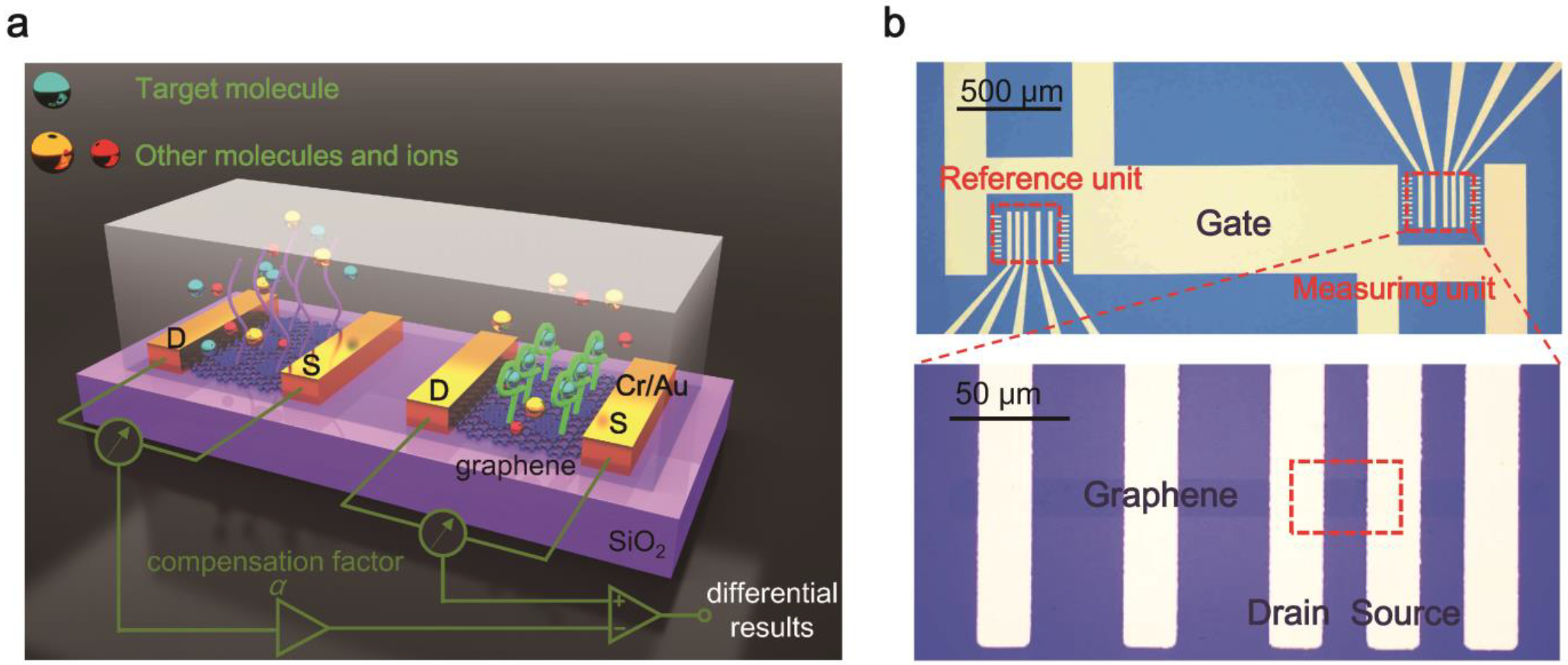
The differential GFET affinity sensor: (a) schematic and (b) optical micrographs.

To introduce the differential measurement method for the sensor, we first consider the transfer characteristics of graphene in the linear regime that can be described by (Kim et al. 2010): I_ds = μ(W/L)C_tot(V_gs−V_ch)V_ds, where μ is the carrier mobility, W/L is the width-to-length of the graphene conducting channel (W/L = 1 in this work), C_tot is the total gating capacitance per unit area, and V_ch is the chemical potential of graphene. This can be used to extract the transconductance (g_m), which represents the change of the (drain-source) current per unit gate voltage:

$$g_m=\frac{\partial I_{\text{ds}}}{\partial V_{\text{gs}}}=\mu (W/L)C_{\text{tot}}{V}_{\text{ds}}$$ (1)

Hence, the transconductance g_m can be calculated for a given value of the gate voltage V_gs.

As the transconductance can describe the sensitivity for graphene sensors (Wang et al. 2016), the extremum value of g_m is a suggested measure of the sensitivity of the graphene because it is commonly used to estimate the carrier mobility and amplification capability of GFETs (Dankerl et al. 2010; Farmer et al. 2009; Liao et al. 2010). On the transconductance curve, the negative extremum (denoted $g_{m,\text{max}}^{-}$) on the hole branch (Wang et al. 2016; also see the shaded region in Fig. 2c below) was selected as a sensitivity indicator for the sensor (and its sensing units) due to the low operating value of V_gs. Since V_ds for the sensing and reference units was set to the same value, we define a compensation factor by

$$\alpha =g_{m,\text{M},\text{max}}^{-}/g_{m,\text{R},\text{max}}^{-}$$ (2)

Since the transconductance represents the change of current per unit voltage and the measuring and reference units were subjected to the same gate voltage, this compensation factor represents the ratio of the current changes of the sensing and reference units. That is, α is a measure of the discrepancies in the responses of the measuring and reference units.

Fig. 2.

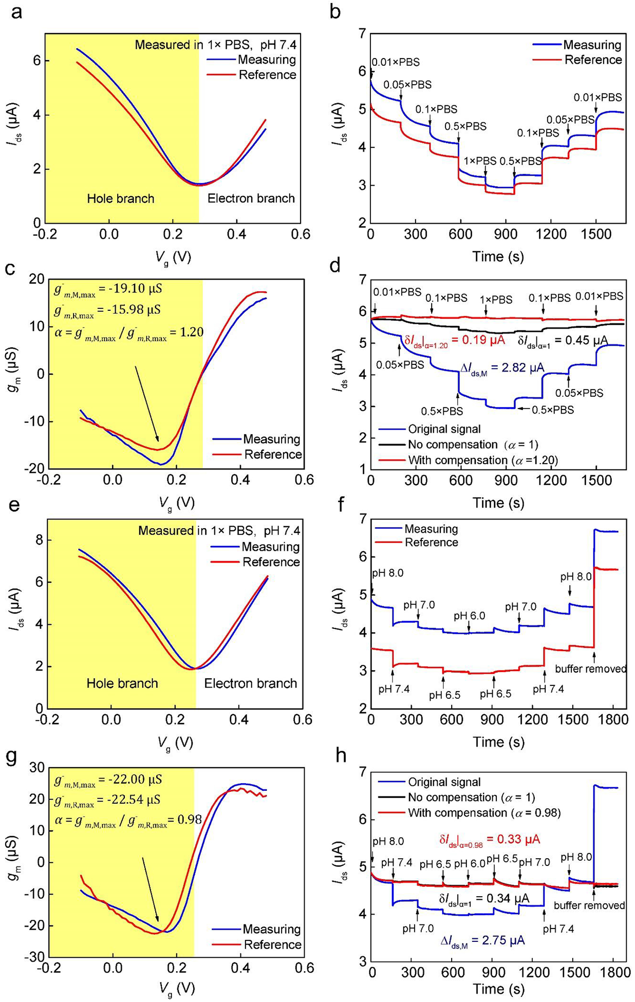
Blank test results in PBS buffer in the presence of interferences. (a)–(d) Ionic strength interference (pH 7.4). (a) Transfer characteristic curves of the sensing and reference units. The majority carrier is holes for data shown in the shaded area. (b) As-measured drain-source current (I_ds) in the presence of ionic strength variations in the units. (c) Transconductance profiles extracted from data shown in (a). $g_{m,\text{M},\text{max}}^{-}$: maximum transconductance of the measuring unit; $g_{m,\text{R},\text{max}}^{-}$: maximum transconductance of the reference unit. The compensation factor (α) was calculated for the hole branch. (d) The drain-source current change (ΔI_ds) for the measuring unit. The current change of the reference unit (ΔI_ds,R) was subtracted from the that of the measuring unit (ΔI_ds,M) by not using (δI_ds|_α=1) and by using compensation (δI_ds|_α=1.20), respectively. (e)–(h) Effects of pH interference (1× PBS). (e) Transfer characteristic curves of the measuring and reference units. (f) As-measured ΔI_ds for the units. (g) Transconductance profiles extracted from data shown in (e). (h) Current change of the measuring unit (ΔI_ds,M) and the differential sensor response (δI_ds|_α=1 and δI_ds|_α=0.98) as described in (d).

In response to an external influence (e.g., exposure to a target analyte or an interfering factor such as ionic strength or pH variation), a sensor unit will generate a current change: ΔI_ds = I_ds − I_ds0, where I_ds0 and I_ds are the current values before and after the application of the influence. Using the compensation factor, we define the differential sensor response by

$$\delta I_{\text{ds}}=\Delta I_{\text{ds},\text{M}}-\alpha \Delta I_{\text{ds},\text{R}}$$ (3)

where ΔI_ds,M and ΔI_ds,R are current changes of the measuring and reference units, respectively. That is, in this compensation-based differential scheme, the current change of the reference unit is scaled by the compensation factor to account for differences in the properties of the two sensing units. When α = 1, this equation reduces to the differential scheme that does not use compensation, as is common practice for differential sensors (Adducci et al. 2016; Fritz et al. 2002; Huang et al. 2014; Huang et al. 2013). Experimental results below will demonstrate that the compensation-based differential scheme can effectively reduce the effects of interferences (e.g., ionic strength and pH variations) on the sensor accuracy.

2.2. Device Fabrication

The standard MEMS fabrication procedure was used for the device fabrication. Briefly, the gate, drain and source electrodes were patterned onto the 285 nm SiO₂/Si substrate through photolithography. Then the patterned electrodes were deposited with Cr/Au (3 nm/40 nm) using electron beam evaporation (AJA International Orion 8E) followed by the lift-off process. Then the monolayer CVD graphene was transferred onto the substrate to bridge the appropriate electrodes using wet etching (Suk et al. 2011) and then patterned (line width: 20 μm) using the oxygen plasma (IoN 40 Plasma System, 120 W, 500 mTorr, 3 min). Finally, all the photoresist on the graphene was removed using Remover PG (Micro Chem).

For microfluidic channels, a photoresist (Micro Chem, SU-8 2075) was used to fabricate a mold on a Si wafer with a height of 150 μm. The PDMS precursor and the curing agent were mixed at a 10:1 ratio and then poured onto the mold. After vacuum degassing and baking on a hotplate (72°C for 45 min), the PDMS was peeled off the SU-8 mold. Finally, the PDMS surface was treated using oxygen plasma (IoN 40 Plasma System, 120 W, 500 mTorr, 20 s), and then bonded onto the substrate surface.

2.3. Characterization and Testing Procedure

Raman spectrum, X-ray photoelectron spectroscopy spectrum, and electrical measurement were utilized to characterize each functionalization process on the graphene sensor (Fig. S2). During all electrical measurements, the gate voltage (V_gs) and the drain-source voltage (V_ds) were supplied using digital SourceMeters (Keithley 2400, Tektronix). Each SourceMeter was connected in one drain-source loop through testing probes. The drain-source current (I_ds) was measured concurrently when V_ds was supplied. As the measuring and reference units shared the gate electrode, V_gs modulated both units simultaneously at the same value. In order to collect current measurements in real-time, the gate voltage was set to V_gs = 0 V. V_ds was fixed at 10 mV to limit I_ds, preventing the risk of damaging the device. All the measurements were controlled and recorded through a Labview program.

2.4. Materials and Reagents

All single-strained DNA (E2 aptamer sequence 5’-NH₂-AAG GGA TGC CGT TTG GGC CCA AGT TCG GCA TAG TG-3’ and random sequence 5’-NH₂-ACG GGT GGC CGC CAG GTC TTG AAG TGG CAG TAT TA-3’) was purchased from Integrated DNA Technologies (Coralville, IA) and purified using HPLC. The testing buffer, 0.05 × phosphate buffered saline (0.05 × PBS, pH 7.4), with 5% dimethyl sulfoxide (DMSO, Sigma-Aldrich), was diluted and adjusted from 1 × PBS (Life Technologies). All analytes were dissolved, separately, in DMSO for 5 mM as stocking solutions and diluted with testing buffer or tap water for variable concentrations.

3. Results and Discussion

3.1. Blank Test

To assess the effectiveness of the compensation-based differential measurement scheme for the minimization of environmental interferences on analyte detection, we first carried out blank tests in PBS buffer solutions without analytes. Since the ionic strength and the pH value are the most important fluctuating parameters in the aquatic environment, we intentionally changed the ionic strength and pH to test this compensation-based differential scheme. We first adjusted PBS buffer (1 × PBS, pH 7.4, ionic strength ~ 163.65 mM) to different ionic strengths (0.01 × PBS, 0.05 × PBS, 0.1 × PBS, 0.5 × PBS). Fig. 2a showed the transfer characteristic curves of graphene of the measuring and reference units, and these two curves did not fully overlap with each other. Moreover, the real-time current responses (I_ds) in the two units in the presence of variations in ionic strength (Fig. 2b), while exhibiting the same trend that is in agreement with results from previously reported GFETs (He et al. 2012), differed quantitatively. For example, consider a current change due to a change of buffer concentration (i.e., ionic strength) as shown in Fig. 2b: ΔI_ds = I_ds − I_ds|_t=0, where I_ds|_t=0 is the current value at time t = 0 (the instant when the sensor was exposed to 0.01×PBS), and I_ds is the approximate equilibrium current value at a given buffer concentration. For example, ΔI_ds|_1×PBS = I_ds|_1×PBS − I_ds|_t=0, where I_ds|_1×PBS is the approximate equilibrium current during the sensor’s exposure to 1×PBS (achieved at t = 900 s). This current change was (ΔI_ds,M)|_1×PBS = 2.82 μA for the measuring unit (blue curve), and (ΔI_ds,R)|_1×PBS = 2.37 μA for the reference unit (red curve).

First, it is important to note that the sensor would give a significant nonzero output of (ΔI_ds,M)|_1×PBS = 2.82 μA if used non-differentially. Since buffer changes are considered as interferences to the specific detection of target analytes and this output should ideally be zero, the sensor operating non-differentially would incur a rather large error. This error can be reduced by differential measurement. In particular, if using the non-compensated differential scheme (α = 1 in Equation (3)), we obtain ΔI_ds,M − ΔI_ds,R = 0.45 μA. Thus, if using this differential current as the sensor output, the measurement error would be reduced by 84%. Below we show that this error reduction can be further improved using the compensation-based differential scheme (Equation (3) with α defined by Equation (2)).

We first consider the effectiveness of the compensation factor in representing differences of the measuring and reference units. Continuing to focus on the current change for 1×PBS (ΔI_ds|_1×PBS), we noted above that (ΔI_ds,M)|_1×PBS = 2.82 μA and (ΔI_ds,R)|_1×PBS = 2.37 μA for the measuring and reference units, respectively. These indicate that there are significant differences between the two units (even though their designs were identical), and the ratio of the current change values was (ΔI_ds,M)|_1×PBS/(ΔI_ds,R)|_1×PBS = 1.19. Now, using Equation (2) (with transconductance given in Fig. 2c), the compensation factor was calculated: α = 1.20, which is well in agreement with the current change ratio. This shows that the compensation factor appropriately captures differences between the measuring and reference units that arise from the fabrication process and material property variations.

It is also interesting to examine the consistency of the compensation factor at different ionic strengths. This is achieved by considering the standard deviation of the values of α obtained at different ionic strengths. For measurement data given in Fig. 2c, this standard deviation was determined to be 0.01 for α values at all of the buffer concentrations tested (Fig. S3). Thus, it was concluded that the compensation factor did not change significantly with the ionic strength variations and remained highly consistent.

Using the compensation factor, we evaluated the compensation-based differential scheme. Again focus on 1×PBS (Fig. 2b) with α = 1.20, Equation (3) was used to obtain δI_ds|_1×PBS = 0.19 μA. This is a 93% reduction from (ΔI_ds,M)|_1×PBS = 2.82 μA if the sensor was used non-differentially, and a further 58% reduction from the aforementioned differential current change without compensation (0.45 μA). The ability of the compensation-based differential scheme to effectively reduce the effects of ionic strength variations on the sensor response can also be seen at other buffer concentrations (Fig. 2d, where the differential response curves have been translated such that they coincide with the as-measured measuring unit current change ΔI_ds,M at time zero).

Finally, in the presence of interferences of pH variations, results similar to those from the blank test with ionic strength interferences are shown in Fig. 2e–h, which also consistently demonstrate that using the compensation-based differential scheme can significantly and more effectively compensate for the effects of measuring and reference unit differences (arising from fabrication and material properties) on the ability of differential measurements to minimize the impact of environmental interferences. Thus, the compensation-based differential scheme will be used throughout analyte detection below unless otherwise noted.

3.2. Detection of E2 in Buffer

We tested this sensor for the selective detection of the pollutant E2, and all measurements were based on three different devices. Based on the affinity binding between E2 molecules and aptamers, the structure change of aptamers would result in a redistribution of charge on the graphene surface (Fig. S4), and I_ds would change, correspondingly. We first used the sensor to detect E2 in the testing buffer, a conditioned media, where the E2 concentration was the only variable. The I_ds values in the measuring and reference units (Fig. 3a) were obtained concurrently and plotted using the current change ΔI_ds=ΔI_ds(t)−ΔI_ds(0), where I_ds(t) is the current at time t and I_ds(0) is the current when t = 0. For each concentration, it took approximately 5 min for the response to achieve the approximate equilibrium. ΔI_ds for the measuring unit (blue curve) increased due to the change of E2 concentrations, while ΔI_ds for the reference unit (red curve) only showed more modest fluctuations which could be the result of surface disturbances when there the sample solution was replenished. To further verify the binding between aptamers and E2 molecules, the transfer characteristic curves of the measuring unit were measured at the concentrations of 0 and 5000 nM (Fig. 3b). At 5000 nM, the curve shifted to the right, and the current on the hole branch was also higher when compared to the case of 0 nM. These changes confirmed the p-type doping of the graphene and the specific binding between the aptamer and E2 molecules. Further, the $g_{m,\text{max}}^{-}$ values in the measuring unit at these two concentrations were calculated. The value slightly decreased from −22.64 to −22.70 μS, implying that the transconductance value on the hole branch remained stable as reported in other related work (Hao et al. 2017).

Fig. 3.

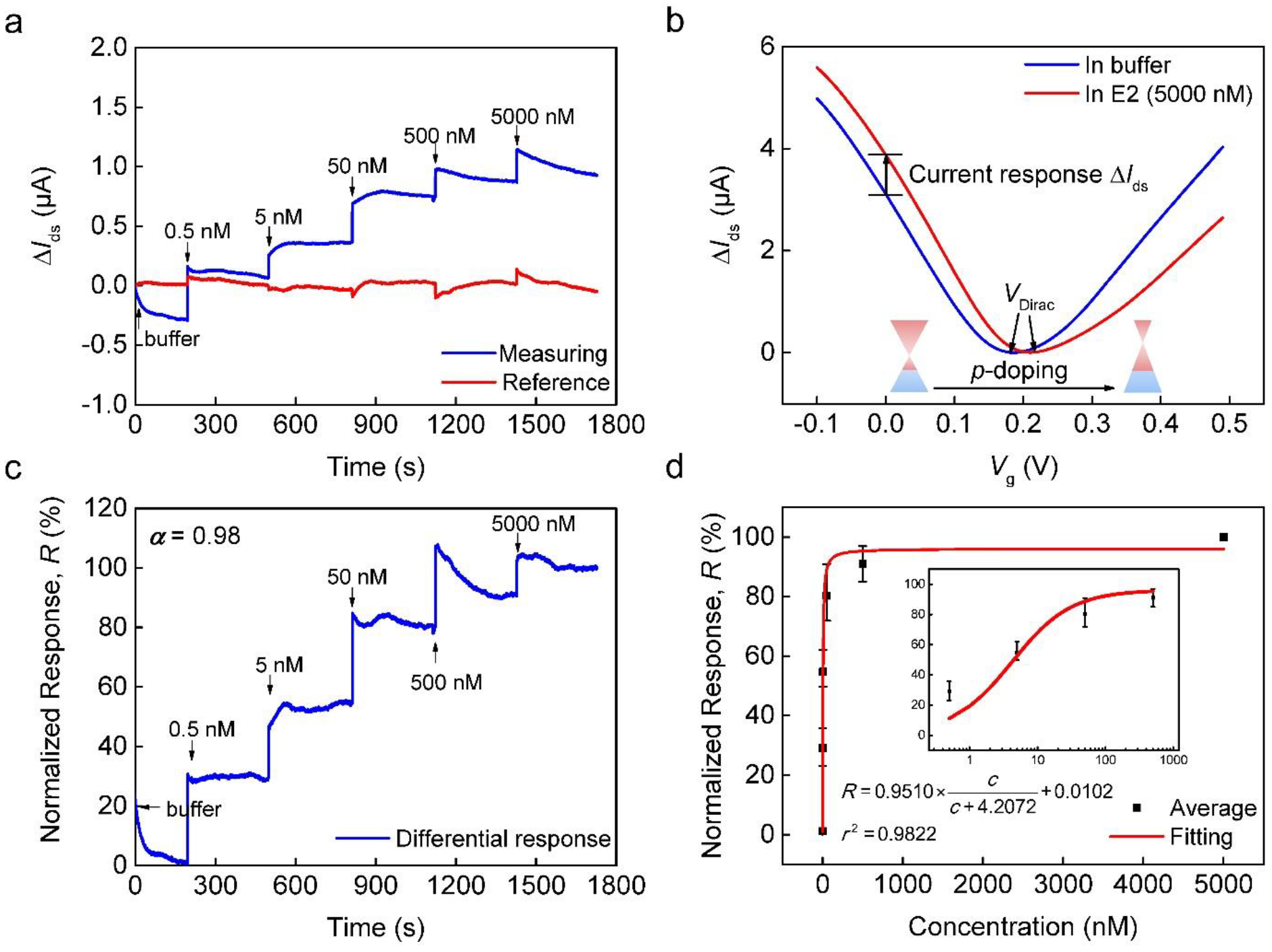
Detection of 17β-estradiol (E2) in testing buffer without interferences. (a) As-measured drain-source current change ΔI_ds at varying E2 concentrations. (b) Transfer characteristic curves of the measuring unit at two different E2 concentrations. (c) Normalized differential responses extracted from data shown in (a) using compensation. (d) Normalized equilibrium response shown as a function of E2 concentration and fitted to the Langmuir equation. Inset: the response plotted on a logarithmic scale for the E2 concentration from 0.5 to 500 nM.

To reduce the impact of fluctuations during testing due to replenishment of samples with different concentrations in the measuring unit and also to account for device-to-device variations of sensor properties, the differential sensor response (Equation (3)) is normalized as follows:

$$R=\left({\delta I_{\text{ds}}-{\delta }_{\text{ds}}|}_{c=0}\right)/\left({\delta I_{\text{ds}}|}_{c=5000}-{\delta I_{\text{ds}}|}_{c=0}\right)$$ (4)

where δI_ds|_c=0 and δI_ds|_c=5000 are the differential response at an analyte concentration of 0 and 5000 nM, respectively. This normalized sensor response is computed for the data in Fig. 3a, and is shown in Fig. 3c. The approximate equilibrium normalized responses at each E2 concentration (i.e., the value of the real-time normalized response, as shown in Fig. 3c, at a sufficiently large time) were further obtained and are depicted in Fig. 3d (6 data points), with the inset providing a zoom-in view of the normalized response (on logarithmic scale) for an E2 concentration range of 0.5 to 500 nM. These normalized responses as a function of E2 concentration were fitted to the Langmuir equation R=δI_ds,max(c/(c+K_D))+D, where D is the overall offset reflecting the response to the pure buffer (Ohno et al. 2010). This allowed the determination of the equilibrium dissociation constant (K_D = 4.21 nM). In addition, the LOD, defined as three times the standard deviation of E2 concentration measurements and determined based on the noise level of the sensor response (σ = 0.0023), was estimated to be 37.26 pM using a method described elsewhere (Li et al. 2017). This LOD is appropriate for detecting E2 in the aquatic environment (Huang et al. 2015). Finally, the specificity of E2 detection by the sensor was confirmed by testing on E2 analog molecules as well as other common endocrine disrupting chemicals (details are described in Supplementary Information).

Next, we introduced an intentionally imposed interference, the pH variation, to the detection process. The testing samples were titrated to different pH values (pH = 6.5, 7.4, 8.0) using NaOH or HCl solution while the other detection conditions were kept the same. As shown in Fig. 4a, current signals in the measuring and reference units responded to pH variations; hence, the response in the measuring unit can be regarded as the combined signal arising from the E2 binding and the pH interference. Notably, the current dropped suddenly when 5000 nM, a higher concentration, was detected due to the pH interference. To reduce the signal caused by pH variations, the same differential sensing scheme was thus implemented. Fig. 4b depicts the normalized sensor response. The signal from pH interferences was reduced, and δI_ds changed in accordance with the change of E2 concentration. We also fitted the result to the Langmuir equation (Fig. 4c) and obtained the equilibrium dissociation constant (K_D = 4.67 nM) and the limit of detection (LOD = 34.70 pM). They were consistent with the values obtained in the absence of interferences, demonstrating that satisfactory detection results could be obtained using our differential sensor even in the presence of pH interferences. Since the pH value in the aquatic environment could fluctuate with time, this interference emulates situations that could result in false responses in water monitoring, which can be rejected by our device.

Fig. 4.

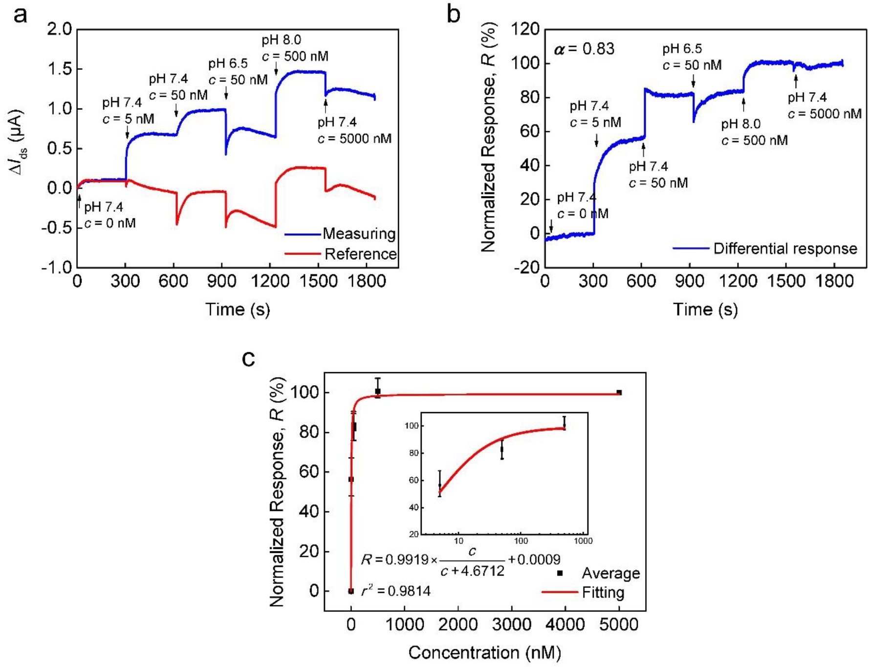
Detection of E2 in buffer in the presence of pH interferences. (a) As-measured ΔI_ds at varying E2 concentrations in the presence of variations in pH. (b) Normalized differential responses extracted from data shown in (a) using compensation. (c) Normalized equilibrium response shown as a function of E2 concentration and fitted to the Langmuir equation. Inset: the response plotted on a logarithmic scale for the E2 concentration from 5 to 500 nM.

3.3. Detection of E2 in Tap Water

We performed detection of E2 in tap water. Tap water is highly relevant to human health as its direct consumption by people is common; yet it contains a large number of chemicals (e.g., transformation products or chemicals that remain after water treatment) (Escher et al. 2013) and is complex. We prepared testing samples by spiking tap water using E2 stocking solution. Transfer characteristic curves were measured in both tap water and testing buffer (Fig. 5a). We noticed that graphene obtained heavier p-type doping in tap water according to the right shift of V_Dirac as shown in Fig. 5a. Moreover, ΔI_ds values for the units increased when tap water (c = 0) was introduced to replenish testing buffer (Fig. 5b). Since the pH value of the tap water was similar to that of the testing buffer (pH 7.3 and 7.4, respectively), it is possible that the different ionic strength in the tap water might have caused this interference. Using the differential sensing scheme (Fig. 5c), the current change, caused by the replenishment of the sensing media (as an ionic strength interference), was reduced. Further, the results were fitted to the Langmuir equation, and the equilibrium dissociation constant (K_D = 27.2 nM) and the limit of detection (LOD = 757.6 pM) were obtained and compared (Fig. 5d). It was found that K_D and LOD were both larger than the corresponding values obtained in the testing buffer. Also, the difference between δI_ds|_c=0 and δI_ds|_c=5000 (~0.10 μA) in Fig. 5b was one order of magnitude less than that (~1.00 μA) in Fig. 3a and 4a, which implies the sensitivity was different when tap water was used. These differences could be related to the lower ionic strength of tap water than that of the buffer. This would cause the Debye length to increase (Pacios et al. 2012) and the strongly charged aptamer molecules to remain inside the electrical double layer before and after they bind to the E2 molecules. Hence the aptamer-E2 binding would result in less charge redistribution in tap water than that in testing buffer.

Fig. 5.

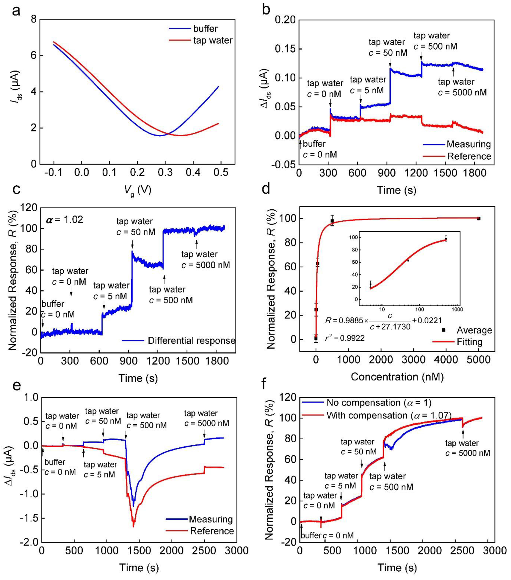
Detection of E2 detection in tap water. (a) Transfer characteristic curves measured in tap water and buffer. (b) As-measured ΔI_ds at varying E2 concentrations. (c) Normalized differential responses extracted from data shown in (b) using compensation. (d) Normalized equilibrium response shown as a function of E2 concentration. The data were fitted to the Langmuir equation. Inset: the response plotted on a logarithmic scale for the E2 concentration from 5 to 500 nM. (e) As-measured ΔI_ds at varying E2 concentrations. When E2 (500 nM) was introduced, a current change occurred for both the measuring and reference units possibly due to unknown interferences in the tap water. (f) Normalized differential responses using (blue curve) and not using compensation (red curve), respectively.

Fig. 5e shows an additional set of measurement results in tap water. Noting that ΔI_ds decreased and then increased within 20 min after the 500 nM sample was introduced. Since this observable interference was not intentionally imposed, we suspect some unknown interferences in tap water might have caused this variation (e.g., non-specific adsorption), and that the current change might display the adsorption and desorption processes. Although the interference source is unknown, we can still implement the differential sensing scheme for the result. It was apparent that such false response was completely eliminated (Fig. 5f, red curve). Again for comparison, we implemented the differential scheme without compensation. Notably, the unknown interference was only partially minimized (Fig. 5f, blue curve). Therefore, false signals caused by the ionic strength and unknown interferences could be reduced to obtain more accurate detection results using the compensation-based differential scheme.

3.4. Reproducibility

Finally, we examined the reproducibility of our device in the analyte detection. The normalized sensor output did not significantly vary from device to device, as can be seen from the error bars in Figure 3(d), 4(c) and 5 (d). Specifically, the relative standard deviations (RSDs) of the sensor response was within 17.66%. It can be seen that our differential GFET nanosensor offers a comparable reproducibility and a lower LOD to other methods in the presence of nonspecific interferences as shown in Table 1.

Table 1.

Comparison of the response characteristics of the nanosensor and other detection methods

Receptor	Analytical techniques	LODa (M)	RSDb(%)	Reference
Aptamer	Fluorescence	3.75×10−9	≤2.91%	(Qi et al. 2018)
Aptamer	Fluorescence	2.1×10−9	≤5%	(Yildirim et al. 2012)
Aptamer	Fluorescence	3.7×10−8	≤10.1%	(Huang et al. 2016)
Antibody	Surface-enhanced Raman Scattering	2.4×10−12	≤20%	(Wang et al. 2016)
Aptamer	Surface-enhanced Raman Spectroscopy	5×10−14	≤27.6%	(Liu et al. 2018)
Polymer	Electrochemistry	2×10−8	≤8%	(Lahcen et al. 2017)
Polymer	Electrochemistry	2.76×10−9	≤3.9%	(Han et al. 2016)
Antibody	Electrochemistry	3.7×10−11	≤15.4%	(Wang et al. 2018)
Aptamer	Colorimetry	2.00×10−10	-	(Alsager et al. 2015)
Aptamer	Photoelectrochemistry	3.3×10−16	≤7.4%	(Du et al. 2017)
Aptamer	Field-effect transistor	5×10−8	-	(Zheng et al. 2015)
Aptamer	Field-effect transistor	3.47×10−11	≤17.66%	This work

^aDetection limit;

^bRelative standard deviation.

4. Conclusion

In this paper, we presented a differential GFET affinity sensor for the selective detection of water pollutants in the presence of nonspecific disturbances and demonstrated the compensation-based differential scheme by the detection of the water pollutant 17β-estradiol (E2) in buffer solution and tap water. This differential design offered an effective rejection of fluctuations in the sensor’s environmental conditions and allowed selective detection of water pollutants. An effective compensation scheme was used to mitigate the impact of variations of fabrication processes and material properties on the differential sensor operation. In the detection of E2, signals originating from pH variations were effectively reduced, allowing E2 to be detected at concentrations ranging from 5 to 5000 nm with a limit of detection of LOD = 34.70 pM and an equilibrium dissociation constant of K_D = 4.67 nM. These results were consistent with those from interference-free detection, for which LOD = 37.26 pM and K_D = 4.21 nM. Moreover, in tap water, where unknown interferences were present, E2 was detected with LOD = 757.6 pM and K_D = 27.2 nM. These results demonstrated that the differential graphene affinity sensor was capable of effectively mitigating the effects of nonspecific interferences. While we focused on tap water as an example of a practically important form of complex water samples, our future work would address the application of the differential graphene nanosensors to surface water (e.g., river and lake) samples, which generally contain even more complex interfering molecules. Such studies would eventually allow us to fully test the potential utility of the differential sensors for water quality monitoring.

Highlights:

• An integrated differential graphene affinity sensor based on field-effect transistors.

• First demonstration of the selective detection of analytes in the presensce of nonspecific disturbances using a graphene sensor.

• A compensation scheme mitigating the impact of fabrication process and material property variations on differential sensing, addressing the challenge for developing differential graphene electronic sensors.

• A compensation-based differential scheme for accurate nanosensing.

References:

- Adducci BA, Gruszewski HA, Khatibi PA, Schmale DG, 2016. Biosens. Bioelectron 78, 160–166. [DOI] [PubMed] [Google Scholar]
- Alsager OA, Kumar S, Zhu B, Travas-Sejdic J, McNatty KP, Hodgkiss JM, 2015. Anal. Chem 87(8), 4201–4209. [DOI] [PubMed] [Google Scholar]
- Dankerl M, Hauf MV, Lippert A, Hess LH, Birner S, Sharp ID, Mahmood A, Mallet P, Veuillen J, Stutzmann M, Garrido JA, 2010. Adv. Funct. Mater 20(18), 3117–3124. [Google Scholar]
- Du X, Dai L, Jiang D, Li H, Hao N, You T, Mao H, Wang K, 2017. Biosens. Bioelectron 91, 706–713. [DOI] [PubMed] [Google Scholar]
- Escher BI; van Daele C; Dutt M; Tang JYM; Altenburger R, 2013. Environ. Sci. Technol 47, 7002–7011. [DOI] [PubMed] [Google Scholar]
- Fan L, Zhao G, Shi H, Liu M, Wang Y, Ke H, 2014. Environ. Sci. Technol 48(10), 5754–5761. [DOI] [PubMed] [Google Scholar]
- Farmer DB, Chiu H, Lin Y, Jenkins KA, Xia F, Avouris P, 2009. Nano Lett. 9(12), 4474–4478. [DOI] [PubMed] [Google Scholar]
- Fritz J, Cooper EB, Gaudet S, Sorger PK, Manalis SR, 2002. Proc. Natl. Acad. Sci. U. S. A 99(22), 14142–14146. [DOI] [PMC free article] [PubMed] [Google Scholar]
- Han Q, Shen X, Zhu W, Zhu C, Zhou X, Jiang H, 2016. Biosens. Bioelectron 79, 180–186. [DOI] [PubMed] [Google Scholar]
- Hao Z, Zhu Y, Wang X, Rotti PG, DiMarco C, Tyler SR, Zhao X, Engelhardt JF, Hone J, Lin Q, 2017. ACS Appl. Mater. Interfaces 9(33), 27504–27511. [DOI] [PMC free article] [PubMed] [Google Scholar]
- He RX, Lin P, Liu ZK, Zhu HW, Zhao XZ, Chan HLW, Yan F, 2012. Nano Lett. 12(3), 1404–1409. [DOI] [PubMed] [Google Scholar]
- Huang B, Sun W, Li X, Liu J, Li Q, Wang R, Pan X, 2015. Ecotox. Environ. Safe 112, 169–176. [DOI] [PubMed] [Google Scholar]
- Huang H, Shi S, Gao X, Gao R, Zhu Y, Wu X, Zang R, Yao T, 2016. Biosens. Bioelectron 79, 198–204. [DOI] [PubMed] [Google Scholar]
- Huang X, Leduc C, Ravussin Y, Li S, Davis E, Song B, Li D, Xu K, Accili D, Wang Q, Leibel R, Lin Q, 2014. Lab Chip 14(2), 294–301. [DOI] [PMC free article] [PubMed] [Google Scholar]
- Huang X, Li S, Davis E, Leduc C, Ravussin Y, Cai H, Song B, Li D, Accili D, Leibel R, Wang Q, Lin Q, 2013. J. Micromech. Microeng 23(5), 55020. [DOI] [PMC free article] [PubMed] [Google Scholar]
- Janssens G, Mangelinckx S, Courtheyn D, Prévost S, De Poorter G, De Kimpe N, Le Bizec B, 2013. J. Agr. Food Chem 61(30), 7242–7249. [DOI] [PubMed] [Google Scholar]
- Kidambi PR, Boutilier MSH, Wang L, Jang D, Kim J, Karnik R, 2017. Adv. Mater 29(19), 1605896. [DOI] [PubMed] [Google Scholar]
- Kim BJ, Jang H, Lee S, Hong BH, Ahn J, Cho JH, 2010. Nano Lett. 10(9), 3464–3466. [DOI] [PubMed] [Google Scholar]
- Lahcen AA, Baleg AA, Baker P, Iwuoha E, Amine A, 2017. Sens. Actuators, B 241, 698–705. [Google Scholar]
- Lei Y, Xiao M, Li Y, Xu L, Zhang H, Zhang Z, Zhang G, 2017. Biosens. Bioelectron 91, 1–7. [DOI] [PubMed] [Google Scholar]
- Li G, Yu X, Liu D, Liu X, Li F, Cui H, 2015. Anal. Chem 87(21), 10976–10981. [DOI] [PubMed] [Google Scholar]
- Li P, Liu B, Zhang D, Sun Y, Liu J, 2016. Appl. Phys. Lett 109(15), 153101. [Google Scholar]
- Li Y, Wang C, Zhu Y, Zhou X, Xiang Y, He M, Zeng S, 2017. Biosens. Bioelectron 89, 758–763. [DOI] [PubMed] [Google Scholar]
- Liang Y, Yu L, Yang R, Li X, Qu L, Li J, 2017. Sens. Actuators, B 240, 1330–1335. [Google Scholar]
- Liao L, Bai J, Qu Y, Lin YC, Li Y, Huang Y, Duan X, 2010. Proc. Natl. Acad. Sci. U. S. A 107(15), 6711–6715. [DOI] [PMC free article] [PubMed] [Google Scholar]
- Liu S, Cheng R, Chen Y, Shi H, Zhao G, 2018. Sens. Actuators, B 254, 1157–1164. [Google Scholar]
- Lupina G, Kitzmann J, Costina I, Lukosius M, Wenger C, Wolff A, Vaziri S, Östling M, Pasternak I, Krajewska A, Strupinski W, Kataria S, Gahoi A, Lemme MC, Ruhl G, Zoth G, Luxenhofer O, Mehr W, 2015. ACS Nano 9(5), 4776–4785. [DOI] [PubMed] [Google Scholar]
- Ma R, Huan Q, Wu L, Yan J, Guo W, Zhang Y, Wang S, Bao L, Liu Y, Du S, Pantelides ST, Gao H, 2017. Nano Lett. 17(9), 5291–5296. [DOI] [PubMed] [Google Scholar]
- Maity A, Sui X, Tarman CR, Pu H, Chang J, Zhou G, Ren R, Mao S, Chen J, 2017. ACS Sens. 2(11), 1653–1661. [DOI] [PubMed] [Google Scholar]
- Mao S, Chang J, Pu H, Lu G, He Q, Zhang H, Chen J, 2017. Chem. Soc. Rev 46(22), 6872–6904. [DOI] [PubMed] [Google Scholar]
- Ohno Y, Maehashi K, Matsumoto K, 2010. J. Am. Chem. Soc 132(51), 18012–18013. [DOI] [PubMed] [Google Scholar]
- Pacios M, Martin-Fernandez I, Borrisé X, Del Valle M, Bartrolí J, Lora-Tamayo E, Godignon P, Pérez-Murano F, Esplandiu MJ, 2012. Nanoscale 4(19), 5917–5923. [DOI] [PubMed] [Google Scholar]
- Pirkle A, Chan J, Venugopal A, Hinojos D, Magnuson CW, McDonnell S, Colombo L, Vogel EM, Ruoff RS, Wallace RM, 2011. Appl. Phys. Lett 99(12), 122108. [Google Scholar]
- Qi X, Hu H, Yang Y, Yunxian P, 2018. Analyst 143 (17), 4163–4170. [DOI] [PubMed] [Google Scholar]
- Shi J, Li X, Chen Q, Gao K, Song H, Guo S, Li Q, Fang M, Liu W, Liu H, Wang X, 2015. Nanoscale 7(17), 7867–7872. [DOI] [PubMed] [Google Scholar]
- Suk JW, Kitt A, Magnuson CW, Hao Y, Ahmed S, An J, Swan AK, Goldberg BB, Ruoff RS, 2011. ACS Nano 5(9), 6916–6924. [DOI] [PubMed] [Google Scholar]
- Tang S, Tong P, You X, Lu W, Chen J, Li G, Zhang L, 2016. Electrochim. Acta 187, 286–292. [Google Scholar]
- Vicarelli L, Heerema SJ, Dekker C, Zandbergen HW, 2015. ACS Nano 9(4), 3428–3435. [DOI] [PMC free article] [PubMed] [Google Scholar]
- Wang C, Kim J, Zhu Y, Yang J, Lee G, Lee S, Yu J, Pei R, Liu G, Nuckolls C, Hone J, Lin Q, 2015. Biosens. Bioelectron 71, 222–229. [DOI] [PMC free article] [PubMed] [Google Scholar]
- Wang C, Li Y, Zhu Y, Zhou X, Lin Q, He M, 2016. Adv. Funct. Mater 26(42), 7668–7678. [Google Scholar]
- Wang R, Chon H, Lee S, Cheng Z, Hong SH, Yoon YH, Choo J, 2016. ACS Appl. Mater. Interfaces 8(17), 10665–10672. [DOI] [PubMed] [Google Scholar]
- Wang Y, Luo J, Liu J, Li X, Kong Z, Jin H, Cai X, 2018. Biosens. Bioelectron 107, 47–53. [DOI] [PubMed] [Google Scholar]
- Wipf M, Stoop RL, Tarasov A, Bedner K, Fu W, Wright IA, Martin CJ, Constable EC, Calame M, Schönenberger C, 2013. ACS Nano 7(7), 5978–5983. [DOI] [PubMed] [Google Scholar]
- Wu G, Dai Z, Tang X, Lin Z, Lo PK, Meyyappan M, Lai KWC, 2017. Adv. Healthcare Mater 6(19), 1700736. [DOI] [PubMed] [Google Scholar]
- Xu S, Jiang S, Zhang C, Yue W, Zou Y, Wang G, Liu H, Zhang X, Li M, Zhu Z, Wang J, 2018. Appl. Surf. Sci 427, 1114–1119. [Google Scholar]
- Xu X, Zhang Z, Qiu L, Zhuang J, Zhang L, Wang H, Liao C, Song H, Qiao R, Gao P, Hu Z, Liao L, Liao Z, Yu D, Wang E, Ding F, Peng H, Liu K, 2016. Nat. Nanotechnol 11(11), 930–935. [DOI] [PubMed] [Google Scholar]
- Yildirim N, Long F, Gao C, He M, Shi H, Gu AZ, 2012. Environ. Sci. Technol 46(6), 3288–3294. [DOI] [PubMed] [Google Scholar]
- Zheng HY, Alsager OA, Wood CS, Hodgkiss JM, Plank NOV, 2015. J. Vac. Sci. Technol., B: Nanotechnol. Microelectron. : Mater., Process., Meas., Phenom 33(6), 6F904. [Google Scholar]
Associated Data
This section collects any data citations, data availability statements, or supplementary materials included in this article.