Mathematical analysis of spread and control of the novel corona virus (COVID-19) in China

Abstract

Number of well-known contagious diseases exist around the world that mainly include HIV, Hepatitis B, influenzas etc., among these, a recently contested coronavirus (COVID-19) is a serious class of such transmissible syndromes. Abundant scientific evidence the wild animals are believed to be the primary hosts of the virus. Majority of such cases are considered to be human-to-human transmission, while a few are due to wild animals-to-human transmission and substantial burdens on healthcare system following this spread. To understand the dynamical behavior such diseases, we fitted a susceptible-infectious-quarantined model for human cases with constant proportions. We proposed a model that provide better constraints on understanding the climaxes of such unseen disastrous spread, relevant consequences, and suggesting future imperative strategies need to be adopted. The main features of the work include the positivity, boundedness, existence and uniqueness of solution of the model. The conditions were derived under which the COVID-19 may extinct or persist in the population. Sensitivity and estimation of those important parameters have been carried out that plays key role in the transmission mechanism. To optimize the spread of such disease, we present a control problem for further analysis using two control measures. The necessary conditions have been derived using the Pontryagin’s maximum principle. Parameter values have been estimated from the real data and experimental numerical simulations are presented for comparison as well as verification of theoretical results. The obtained numerical results also present the verification, accuracy, validation, and robustness of the proposed scheme.

1. Introduction

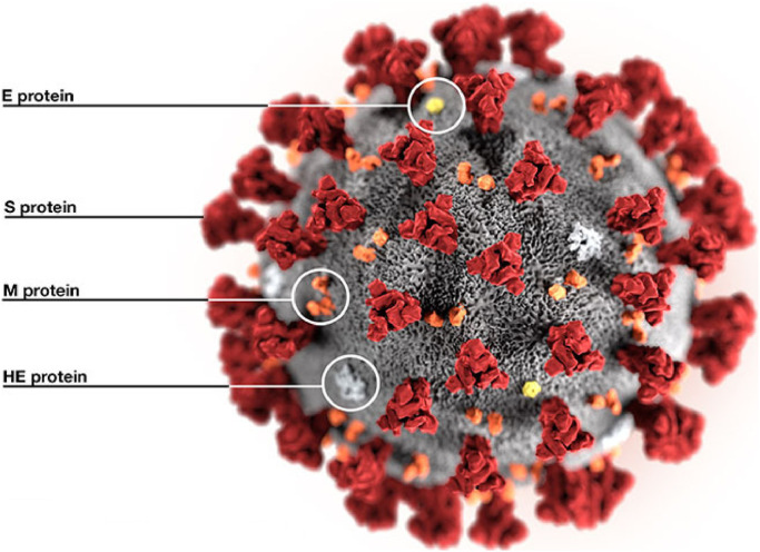
On the basis of genetic properties the coronaviranae family comprises of four genera, which include genus Betacoronavirus, genus Gammacoronavirus and genus Deltacoronavirus etc., [1]. RNA genome of the coronavirus is the largest RNA among the all reported virus RNA ranging from 26 to 32 kb [2]. The coronavirus can infect aves reptiles mammals including homo sapiens. The coronavirus mainly infect subclinical [1], [2], [3]. The severe respiratory syndrome (SARS-CoV) and Middle East respiratory syndrome coronavirus (MERS-CoV) are zoonotic pathogens which are related to the genus of Betacoronavirus causing severe respiratory infections in man. The COVID-19 can rapidly adapt to the new host and ecological niches and attain the tendency for genetic recombination and strengthen the inherently mutation rate of typical RNA viruses [4], [5]. The typical structural representation of the COVID-19 is shown in Fig. 1 highlighting various segments of proteins namely E-Protein, S-Protein, M-Protein, and HE-Protein [3].

Fig. 1.

Structure of COVID-19 [3].

Not yet the definite source of this virus is still under consideration. Apart, the infections in family and health workers clusters confirm the spread from human to human, while the mood of transmission is still open for confirmation. However, on January 21, 2020, WHO approved human to human transmission [3], [5], [6].

Till March 16, 2020, a total of 81,009 confirm cases were reported in Mainland China due to pneumonia/COVID-19 and the same time new patients were also reported worldwide including Thailand, South Korea, Japan, United Kingdom, USA, India etc. The COVID-19 appeared to cause mild from viral pneumonia with low capability from person to person transmission which is different from SARS-CoV [4]. The attitude behind this maybe because of the recombination within receptor-binding of glycoprotein of the virus originated form the snake, wildlife or from both. Accordingly, the COVID-19 will likely be attenuated upon infection to humans. Still the concern about the adaptation in humans may acquire more competence to efficiently replicate and provide feasible route transmit rapidly via close contacts with the infected bodies [7].

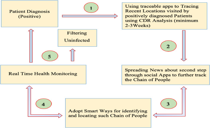
In order to identify the mechanism from which CoVs infected patients are passing, we developed a flow diagram in Fig. 2 . In the first step, an infected patient is identified. Further, we will use any traceable app to track back the record of locations recently visited by the positively diagnosed patients. For this purpose, CDR analysis can be used with minimum $2-3$ weeks of records. Followed by this, the awareness about this disease will be increased among the public. For this aim, we shall spread the news of the result of the second step through social media platforms such as apps. It will also lead to further trace the chain of the infected people. Furthermore, we will use any easiest and possible method to get the chain of people who interacted with patient and the places visited by them. The identified confirmed coronavirus infected patients will comply with strict health and security monitoring. Finally, the same strategy shall be used for all infected patients.

Fig. 2.

COVID-19 patients identification and its protocol.

To properly know the mechanism of transmission and hence control the COVID-19 mathematically, we will formulate a model with the help of available literature. The current study is actually divided into three main parts; the statistic, dynamic and control. In the first part, we just studied the qualitative aspects of the disease and estimated the key rates form the real data. In the dynamics part, the authors have tried to answer questions like when the disease will dies out of the Hubie province? When does it will persist in the population? Which parameters are more responsible for the disease spreading? Mathematically, we will calculate the possible equilibria of the model and its stability analysis will be carried out using the methods of linearization, the Lyapunov theory and geometrical approach. The last part is devoted to control theory of COVID-19. In this part, we have chosen two control measures and formulated a control problem for further mathematical analysis. To obtain an optimal control problem along with characterization of control variables, using the Pontrygin’s principle. The obtained analytical results and real data will be compared with numerical solutions using standard numerical method.

Formal organization of the manuscript are as: In the 2nd section, the statistics analysis of Coronavirus (COVID-19) will be presented. The data to be used for the study is till March 2, 2020. We proposed the Coronavirus (COVID-19) model in Section 3 using the previous knowledge on epidemic modeling. Further, we deliberate the properties of existence, positivity, boundedness of solution to the problem and biologically feasibility. In Section 4, the reproductive number will be calculated and it will be used for analyzing both local and global behavior of the disease free state. The dynamics with local properties as well as global properties around endemic state will be carried out in Section 5. Also, local sensitivity analysis will be a part of this section. In Section 6, we will present numerical simulation for supporting theoretical results related to dynamical behavior of the problem under discussion. Section 7 is devoted to the formulation of the optimal control problem, development of suitable objective functional, existence of control variables, optimality condition and characterization of the control variables. The numerical results will be derived both for control and without control problems and a comparison may be presented between real data and the obtained findings. Finally, Section 8 and 9 will be presented which are discussion and conclusion of the study, respectively.

2. Statistical analysis of COVID-19

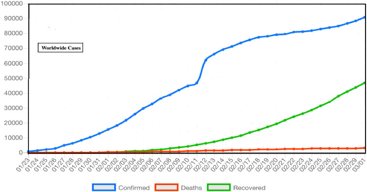
The 2019 novel coronavirus (COVID-19) was identified by using the next-generation sequencing. Until 28th January,2020, about 5900 confirmed cases and about 9000 suspected cased were reported via Chinese authorities due to COVID-19 in various region of Mainland China [7]. In the same time various cases of COVID-19 have been reported in other countries like Italy, Iran, Japan, Spain, USA, Germany, South Korea and Singapore etc. The medical worker and family member were also reported infected causing human to human transmission upon exposure to infected person of COVID-19. The usual symptoms of novel COVID in an infected subject are high fever, some had dyspnea, while the chest radiographs reveals invasive lesions in lungs [5], [6], [7]. The epidemiological curve in Fig. 3 for the worldwide case reported and upon data implementation, can suggests the trend of infected, death and recovered cases from COVID-19.

Fig. 3.

Daily new number of epidemiological curve of COVID-19 (infected, deaths, recovered) worldwide.

On December 31, 2019 Wuhan health authority release a public notice about the outbreak after confirmation, with no evidence from human to human transmission of the virus and suggest that the disease is preventable and controllable after implementing proper precautionary measurements while going out. The WHO was also formally informed about the outbreak shortly [7]. Later on January 20, 2020 scientists from the China’s National Health Commission expressed their potential from one human to another upon the confirmation of two cases in Guangdong, upon the visit of infected family visited to Wuhan. Later the Wuhan authorities also announced new measurements for the control and prevention of this epidemic by canceling Chinese New Year celebrations, and start examine of body temperature upon traveling in public transport on 14th January, 2020. Beside all these for the general public safeguard a quarantine period was introduce on January 23rd, 2020 and lock-down Wuhan was initiated [7], [8].

On January 26th, 2020, a high level tasked force was initiated for the prevention and control of newly rise epidemic by COVID-19, which decided to implement new measurements for the control and prevention aiding extension of spring festival holidays [9]. Besides on 1st February, Huanggang, Hubei authorities permitted single person for purchasing necessary household items on alternative days. Then same measurements was implemented in other parts of the Mainland China. Till 20th of February, 2020, the number of reported cases were 75,465 in China according to NRS [10], [11].

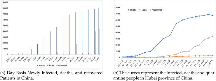
NRS updated the record on daily basis for the cumulative confirmed, as well as suspected, dead and new cases. Beside Hubie, each province hold a media talk at 1300hr daily and update about the CoVID-19 and compare with the previous day [10], [11]. From Fig. 4 a, the curves for epidemics are drawn with the help of Infectious Disease Information System (IDIS) data China’s National, which need every case of covid and therefore have been reported electronically by authorities immediately after diagnosed. It contain cases which are reported as asymptomatic and data is updated in real time, while individually cases are reported and downloaded after every 2400hr. Fig. 4b represents the epidemiological curve of the reported cases of Hubei province. The curves includes the graphical presentation of the infected, death and quarantine cases [5], [6], [7].

Fig. 4.

The daily and total infected, death, recovered and quarantined cases.

3. Corona model formulation

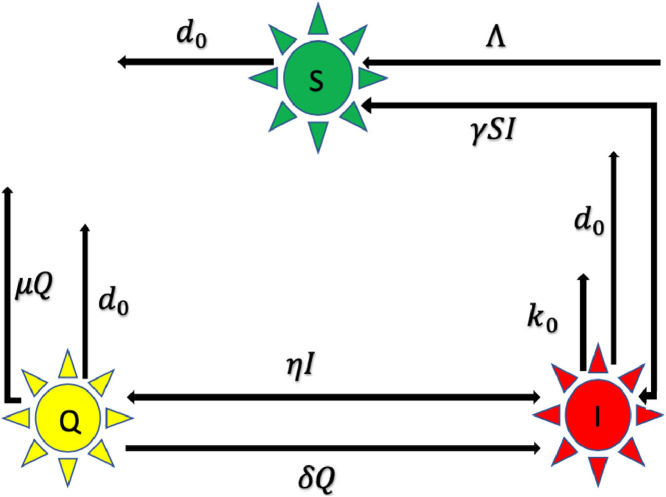
We discuss transmission dynamics of the novel coronavirus a mathematical model according to the component of the virus transmittal [12], [13], [14]. We subdivide the human host populace (T(t)) in three groups: susceptible individuals S(t) as vulnerable for the infection; infected I(t) i.e., confirmed infected; Q(t) those who have contact history with an infectious individual and may or may not be infected with COVID-19 and whose activities have been restricted for a specific period of time. SIQ models are appropriate to model COVID-19 as quarantine destabilizes the epidemic and lead to sustained oscillations in the dynamics of the disease. The COVID-19 model whose the transmission structure is depicted in the Fig. 5 .

Fig. 5.

Flowchart of our proposed model (1).

Moreover, we also put some assumptions before presenting the proposed model in the following form:

• [a ₁.] All parameters as well as variable and state variables are positive as well as non-negative respectively.

• [a ₂.] The susceptible agents goes to the infection classes and there is a constant inflow into the susceptible population.

• [a ₃.] Initially infected or suspected people move to quarantined class and confirmed cases from quarantined come back to the infected compartment.

Keeping in view the 5 and assumptions $a_1-a_3$ we can describe the dynamics of COVID-19 in Hubie in the form of the system of three differential equations:

$$\begin{array}{cc}\frac{d}{dt}S\left(t\right)\hfill & =\Lambda -\gamma S\left(t\right)I\left(t\right)-d_{0}S\left(t\right),\hfill \\ \frac{d}{dt}I\left(t\right)\hfill & =\gamma S\left(t\right)I\left(t\right)-(d_0+k+\eta )I\left(t\right)+\sigma Q\left(t\right),\hfill \\ \frac{d}{dt}Q\left(t\right)\hfill & =\eta I\left(t\right)-(d_0+\mu +\sigma )Q\left(t\right),\hfill \end{array}$$ (1)

with initial conditions

$$S\left(0\right)=S_0>0,I\left(0\right)=I_0\ge 0,Q\left(0\right)=Q_0\ge 0,$$ (2)

where the parameters detail and its associated description are explained in the table. 1 given below.

Table 1.

Model parameters with detailed description.

Notation	Parameters description
Λ	Recruitment rate
γ	Disease transmission rate
d0	Natural death rate
η	Rate of getting quarantine
μ	Disease-related death rate in quarantined individuals
σ	Rate at which quarantined people getting infection
k	Disease death in the infected group

We discuss the well possedness of the proposed model in the form of the following axioms.

Proposition 1

The model (1) in orthant $R_{+}^3$ is invariant.

Proof

Let $Y={(S,I,Q)}^T,$ then system (1) becomes

$$\frac{dY\left(t\right)}{dt}=LY+C,$$ (3)

where

$$\begin{array}{cc}L\hfill & =\left(\begin{array}{ccc}-(\gamma I\left(t\right)+d_0)& 0& 0\\ \gamma I\left(t\right)& -(d_0+k+\eta )& \sigma \\ 0& \eta & -(d_0+\mu +\sigma )\end{array}\right),\hfill \\ C\hfill & =\left(\begin{array}{c}\Lambda \\ 0\\ 0\end{array}\right).\hfill \end{array}$$

Clearly, C ≥ 0 and L preserve the axioms of Metzler matrix, so system (1) is invariant in $R_{+}^3$. □

Proposition 2

The solution of (1) i.e., (S, I, Q) with (2) are positive.

Proof

It could be clearly noted that the solution of the first equation of system (1) becomes

$$\frac{dS\left(t\right)}{dt}+(\gamma I\left(t\right)+d_0)S\left(t\right)=\Lambda .$$ (4)

The solution of Eq. (4) is

$$S\left(t\right)=e^{-{\int }_0^t(\gamma I\left(t\right)+d_0)dt}(S_0+\Lambda \int e^{{\int }_0^t(\gamma I\left(t\right)+d_0)dt}dt),$$ (5)

∀ t > 0, which shows that S(t) > 0. Similarly the second equation of (1) gives the form

$$I\left(t\right)=e^{-{\int }_0^t(d_0+k+\eta -\gamma S\left(t\right))dt}(I_0+\sigma \int Q\left(t\right)e^{{\int }_0^t(d_0+k+\eta -\gamma S\left(t\right))d\tau }dt),$$

which implies that I(t) ≥ 0. Continuing the same process it is very simple to prove that Q(t) is also positive. Thus (S, I, Q) is nonnegative. □

Proposition 3

The solution i.e., (S, I, Q) of the proposed problem is given by (1) – (2) is bounded.

Proof

Since

$$T\left(t\right)=S\left(t\right)+I\left(t\right)+Q\left(t\right).$$ (6)

The differentiation of the above Eq. (6) gives

$$\frac{dT}{dt}+d_{0}T=\Lambda -\mu Q-kI.$$ (7)

Clearly, $\frac{dT}{dt}+d_{0}T\le \Lambda$. Solving we obtain

$$0<T\left(t\right)\le \frac{\Lambda }{d_0}+T\left(0\right)e^{-d_{0}t},$$ (8)

which gives that $0<T(S,I,Q)\le \frac{\Lambda }{d_0}$ as t → ∞. □

Proposition 4

If $T\left(0\right)\le \frac{\Lambda }{d_0},$ then the proposed problem is stated by (1) – (2) is a well-defined dynamical system the region is given by

$$\Delta =\{(S,I,Q)\in {\mathbb{R}}_{+}^3:0<T\le \frac{\Lambda }{d_0}\},$$ (9)

which is biologically feasible. Moreover every solution in Δ remains in Δ for t ≥ 0.

Proof

It is very much clear that all the states variables of the proposed problem are nonnegative, so the problem as stated by (1)–(2) is well-posed and biologically feasible. From $T\left(0\right)\le \frac{\Lambda }{d_0},$ we concludes that $T\left(t\right)\le \frac{\Lambda }{d_0}$. So every solution of (1) along with (2) in Δ remains in Δ. □

4. Basic reproductive number and stability of disease-free equilibrium

Let

$$a=d_0+k+\eta ,b=d_0+\mu +\sigma .$$ (10)

The disease-free state (E ₁) takes the form

$$E_1=(S_1,0,0),S_1=\frac{\Lambda }{d_0}.$$ (11)

This disease free state is used to calculate the threshold parameter (${\mathcal{R}}_0$), also called the basic reproduction number i.e., the average of secondary number of infections, see for detail [15], [16], [17], [18]. Moreover, the threshold parameter (${\mathcal{R}}_0$) is used in the calculating of the endemic state. We follow the Watmough et al., method for the purposes of calculating the threshold parameter, whose detail is given in [14]. We know that I* > 0, so

$$I^{*}=\frac{\gamma \Lambda b-d_{0}ab+d_0\sigma \eta }{ab-\sigma \eta }.$$

By rearranging the terms, we can write I ^⋆ in the following way

$$I^{*}=\frac{b\Lambda \gamma -d_0(b(d_0+k)+\eta (d_0+\mu ))}{\gamma (b(d_0+k)+\eta (d_0+\mu ))}=\frac{d_0}{\gamma }({\mathcal{R}}_0-1).$$ (12)

The term ${\mathcal{R}}_0$ used in (12) and so called the threshold number or threshold quantity which is given by

$${\mathcal{R}}_0=\frac{b\Lambda \gamma }{d_0(b(d_0+k)+\eta (d_0+\mu ))}.$$ (13)

Lemma 1

If ${\mathcal{R}}_0<1$ then model (1) is stable locally at DFE (E ₁ ) defined in (11) .

Proof

The three eigen-values of the Jacobean matrix at DFE are ${\lambda }_1=-d_0,$ ${\lambda }_2=-b$ and ${\lambda }_3=\frac{b(d_0+k)+\eta (d_0+\mu )}{b}({\mathcal{R}}_0-1)-\frac{\eta \sigma }{b}$. Clearly, the first two eigenvalues are negative, whereas, the third eigenvalue is negative only if ${\mathcal{R}}_0<1$. Hence the proof. □

Theorem 1

Assume that ${\mathcal{R}}_0<1,$ then model (1) is stable globally at DFE (E ₁ ) (11) . Otherwise unstable.

Proof

We define a function is given by

$$F\left(t\right)=S_1(\frac{S}{S_1}-\ln \frac{S}{S_1})+I\left(t\right)+Q\left(t\right).$$

Differentiating F(t), we get

$$\begin{array}{cc}\frac{dF}{dt}\hfill & =(\frac{dS}{dt}-\frac{S_1}{S}\frac{dS}{dt})+\frac{dI}{dt}+\frac{dQ}{dt}\hfill \\ & =-\frac{S_1}{S}\frac{dS}{dt}+\frac{dS}{dt}+\frac{dI}{dt}+\frac{dQ}{dt}.\hfill \end{array}$$ (14)

Then

$$\begin{array}{ccc}\hfill \frac{dF}{dt}& & =-\frac{S_1}{S}(\Lambda -\gamma S\left(t\right)I\left(t\right)\hfill \\ & & -d_{0}S\left(t\right))+\Lambda -d_0(S+I+Q)-\mu Q-kI.\hfill \end{array}$$

The simplification and some re-arrangements gives

$$\frac{dF}{dt}=-\frac{(\Lambda -d_{0}S){}^2}{d_{0}S}+\frac{b\Lambda \gamma -d_{0}b(d_0+k)}{b{d}_0}I-(d_0+\mu )Q.$$

As $Q=\frac{\eta }{b}I,$ thus

$$\begin{array}{cc}\frac{dF}{dt}\hfill & =-\frac{{(\Lambda -d_{0}S)}^2}{d_{0}S}+\frac{b\Lambda \gamma -d_{0}b(d_0+k)}{b{d}_0}I-\frac{\eta (d_0+\mu )}{b}I,\hfill \\ & =-\frac{{(\Lambda -d_{0}S)}^2}{d_{0}S}+\frac{b\Lambda \gamma -d_{0}b(d_0+k)-d_0\eta (d_0+\mu )}{b{d}_0}I,\hfill \\ & =-\frac{{(\Lambda -d_{0}S)}^2}{d_{0}S}+\frac{b(d_0+k)+\eta (d_0+\mu )}{b}({\mathcal{R}}_0-1)I.\hfill \end{array}$$

Thus, when ${\mathcal{R}}_0<1,$ then $\frac{dF}{dt}<0$. Also, $\frac{dF}{dt}=0$ iff $S\left(t\right)=S_1,$ $I\left(t\right)=0$ and $Q\left(t\right)=0,$ which proves the conclusion. □

5. Existence and stability of endemic equilibrium

We discuss the endemic state (EE) in this section. To prove the stability of model (1) at endemic equilibrium, let $E_2^{*}$ is the EE and then by the use of Eq. (10) and Eq. (13) we arrive

$$E_2^{*}=(S^{*},I^{*},Q^{*}),$$ (15)

where

$$\begin{array}{cc}{S}^{*}\hfill & =\frac{ab-\sigma \eta }{\gamma b}=\frac{\Lambda }{d_0{\mathcal{R}}_0},\hfill \\ I^{*}\hfill & =\frac{\gamma \Lambda b-d_{0}ab+d_0\sigma \eta }{ab-\sigma \eta }=\frac{d_0}{\gamma }({\mathcal{R}}_0-1),\hfill \\ Q^{*}\hfill & =\frac{\gamma \Lambda b\eta -d_{0}ab\eta -d_0\sigma {\eta }^2}{\gamma a{b}^2-\gamma \sigma b\eta }=\frac{d_0\eta }{b\gamma }({\mathcal{R}}_0-1).\hfill \end{array}$$

Clearly, the relations (15) exists if ${\mathcal{R}}_0>1$.

Lemma 2

If ${\mathcal{R}}_0>1,$ then (15) exists for the problem as stated by (1) .

The local dynamics at EE (15) is discussed via the following theorem.

Theorem 2

If ${\mathcal{R}}_0>1,$ then system (1) is locally asymptotically stable at the endemic equilibrium $E_2^{*}$ defined in (15) . Otherwise, (1) is unstable.

Proof

Let J* is the Jacobian matrix of (1) at $E_2^{*}$ (15), then

$$J^{*}=\left(\begin{array}{ccc}-\gamma I^{*}-d_0& -\gamma S^{*}& 0\\ \gamma I^{*}& \gamma S^{*}-a& 0\\ 0& \eta & -b\end{array}\right).$$ (16)

For obtaining the characteristic polynomail, we set $|J^{*}-\lambda A|$=0, where A is identity matrix. Thus

$$det\left(\begin{array}{ccc}-\gamma I^{*}-d_0-\lambda & -\gamma S^{*}& 0\\ \gamma I^{*}& \gamma S^{*}-a-\lambda & 0\\ 0& \eta & -b-\lambda \end{array}\right)=0.$$ (17)

Expansion of the determinant in (17) gives us

$$\begin{array}{ccc}& & |J^{*}-\lambda A|=\hfill \\ & & -(b+\lambda )[-(\gamma I^{★}+d_0+\lambda )(\gamma S^{★}-a-\lambda )+{\gamma }^2{S}^{★}{I}^{★}]=0,\hfill \end{array}$$

implies that

$$(b+\lambda )[{\lambda }^2-(\gamma S^{★}-a-\gamma I^{★}-d_0)\lambda +a\gamma I^{★}-d_0\gamma S^{★}+a{d}_0]=0.$$

We noted that one of the eigenvalue of the matrix is ${\lambda }_1=-b$. For calculating the values of other eigenvalues, we will consider the quadratic equation

$${\lambda }^2-(\gamma S^{★}-a-\gamma I^{★}-d_0)\lambda +a\gamma I^{★}-d_0\gamma S^{★}+a{d}_0=0.$$

By using the values of the endemic equilibrium, we ca write the above equation in the form

$$\begin{array}{ccc}& & {\lambda }^2+\frac{\sigma \eta +d_{0}b{\mathcal{R}}_0}{b}\lambda \hfill \\ & & +\frac{d_0}{b}(b(d_0+k)+\eta (d_0+\mu ))({\mathcal{R}}_0-1)+\sigma \eta {\mathcal{R}}_0=0\hfill \end{array}$$ (18)

Now by Descartes’ rules of sign, if ${\mathcal{R}}_0>1$ then equation (18) has two negative real roots or complex with negative real parts. Hence all of the eigenvalues are negative and hence the theorem. □

Theorem 3

Assumption of ${\mathcal{R}}_0>1$ guarantees that endemic equilibrium $E_2^{*}=(S^{*},I^{*},Q^{*})$ of model (1) is globally asymptotically stable and unstable otherwise.

Proof

Let J ₂ and $J_2^{\mid 2\mid }$ be the Jacobian matrix and second additive compound matrix of the system containing only the model (1) and using Eq. (10). Then

$$\begin{array}{cc}{J}_2\hfill & =\left(\begin{array}{ccc}-\gamma I\left(t\right)-d_0& -\gamma S\left(t\right)& 0\\ \gamma I\left(t\right)& \gamma S\left(t\right)-(d_0+k+\eta )& \sigma \\ o& \eta & -(d_0+\mu +\sigma )\end{array}\right),\hfill \\ J_2^{\mid 2\mid }\hfill & =\left(\begin{array}{ccc}-\gamma I\left(t\right)-d_0+\gamma S\left(t\right)-a& \sigma & 0\\ \eta & -\gamma I\left(t\right)-d_0-b& -\gamma S\left(t\right)\\ 0& \gamma I\left(t\right)& \gamma S\left(t\right)-a-b\end{array}\right).\hfill \end{array}$$

Next, we will take into account the function $P\left(\chi \right)=P(S,I,Q)=\mathrm{diag}\{\frac{S}{I},\frac{S}{I},\frac{S}{I}\},$ then $P^{-1}\left(\chi \right)=\mathrm{diag}\{\frac{I}{S},\frac{I}{S},\frac{I}{S}\}$. By considering the derivative P_f(χ), we have

$$P_f\left(\chi \right)=\mathrm{diag}\{\frac{\dot{S}}{I}-\frac{S\dot{I}}{I^2},\frac{\dot{S}}{I}-\frac{S\dot{I}}{I^2},\frac{\dot{S}}{I}-\frac{S\dot{I}}{I^2}\}.$$

Thus, $P_f{P}^{-1}=\mathrm{diag}\{\frac{\dot{S}}{I}-\frac{\dot{I}}{I},\frac{\dot{S}}{I}-\frac{\dot{I}}{I},\frac{\dot{S}}{I}-\frac{\dot{I}}{I}\}$ and $P{J}_2^{\mid 2\mid }{P}^{-1}=J_2^{\mid 2\mid }$. Taking

$$B=P_f{P}^{-1}+P{J}_2^{\mid 2\mid }{P}^{-1}.$$

For simplicity, we write B, such that

$$B=\left(\begin{array}{ccc}\frac{\dot{S}}{I}-\frac{\dot{I}}{I}& 0& 0\\ 0& \frac{\dot{S}}{I}-\frac{\dot{I}}{I}& 0\\ 0& 0& \frac{\dot{S}}{I}-\frac{\dot{I}}{I}\end{array}\right)+\left(\begin{array}{ccc}-\gamma I\left(t\right)-d_0+\gamma S-\left(t\right)-a& \sigma & 0\\ \eta & -\gamma I\left(t\right)-d_0-b& -\gamma S\left(t\right)\\ 0& \gamma I\left(t\right)& \gamma S\left(t\right)-a-b\end{array}\right),$$

$$=\left(\begin{array}{ccc}\frac{\dot{S}}{I}-\frac{\dot{I}}{I}-\gamma I\left(t\right)-d_0+\gamma S\left(t\right)-a& \sigma & 0\\ \eta & \frac{\dot{S}}{I}-\frac{\dot{I}}{I}-\gamma I\left(t\right)-d_0-b& -\gamma S\left(t\right)\\ 0& \gamma I\left(t\right)& \frac{\dot{S}}{S}-\frac{\dot{I}}{I}+\gamma S\left(t\right)-d_0-a-b\end{array}\right),$$

$$=\left(\begin{array}{cc}{X}_{11}& X_{12}\\ X_{21}& X_{22}\end{array}\right),$$

where

$$\begin{array}{cc}& X_{11}=\frac{\dot{S}}{I}-\frac{\dot{I}}{I}-\gamma I\left(t\right)-d_0+\gamma S\left(t\right)-a,\hfill \\ \hfill & X_{12}=\left(\begin{array}{cc}\sigma & 0\end{array}\right),X_{21}=\left(\begin{array}{c}0\\ 0\end{array}\right),\hfill \end{array}$$

$$X_{22}=\left(\begin{array}{cc}\frac{\dot{S}}{I}-\frac{\dot{I}}{I}-\gamma I\left(t\right)-d_0-b& -\gamma S\left(t\right)\\ \gamma I\left(t\right)& \frac{\dot{S}}{S}-\frac{\dot{I}}{I}+\gamma S\left(t\right)-a-b\end{array}\right).$$

Let us assume that (X ₁, X ₂, X ₃) be a vector in ${\mathbb{R}}^3$ with the norm ‖ · ‖ defined by

$$\parallel X_1,X_2,X_3\parallel =\max \{\parallel X_1\parallel ,\parallel X_2\parallel +\parallel X_3\parallel \}.$$

Considering the Lozinski measure ℓ(B) [19], [20] with endowed norm defined above

$$\ell \left(B\right)\le \sup \{g_1,g_2\}=\sup \{\ell \left(X_{11}\right)+\parallel X_{12}\parallel ,\ell \left(X_{22}\right)+\parallel X_{21}\parallel \},$$

where $g_i=\parallel X_{ij}\parallel +\ell \left(X_{ii}\right)$ for $i,j=1,2$ and i ≠ j, which implies that

$$g_1=\parallel X_{12}\parallel +\ell \left(X_{11}\right),g_2=\parallel X_{21}\parallel +\ell \left(X_{22}\right),$$

where

$$\begin{array}{cc}\ell \left(X_{11}\right)\hfill & =\frac{\dot{S}}{S}-\frac{\dot{I}}{I}-\gamma I+\gamma S-2d_0-k-\eta ,\hfill \\ \ell \left(X_{22}\right)\hfill & =\frac{\dot{S}}{S}-\frac{\dot{I}}{I}-2d_0-\mu -\sigma .\hfill \end{array}$$

Since, $\parallel X_{12}\parallel =\sigma$ and $\parallel X_{21}\parallel =\eta ,$ therefore, g ₁ and g ₂ becomes

$$\begin{array}{cc}{g}_1\hfill & =\frac{\dot{S}}{S}-\frac{\dot{I}}{I}-\gamma (I-S)-2d_0-k-\gamma -k+\sigma ,\hfill \\ g_2\hfill & =\frac{\dot{S}}{S}-\frac{\dot{I}}{I}-2d_0-\mu -\gamma +\eta .\hfill \end{array}$$ (19)

Thus, we can also write Eq. (19) as

$$\begin{array}{cc}{g}_1\hfill & \le \frac{\dot{S}}{S}-2d_0-k-\eta +\sigma ,\hfill \\ g_2\hfill & \le \frac{\dot{S}}{S}-2d_0-\mu -\eta +\sigma .\hfill \end{array}$$

As a result, we get

$$\begin{array}{cc}\ell \left(B\right)\hfill & \le \sup \{g_1,g_2\},\hfill \\ & \le \sup \{\frac{\dot{S}}{S}-2d_0-min\{k+\eta -\sigma \}\le \frac{\dot{S}}{S}-2d_0,\hfill \\ & ifk+\eta >0and\mu +\sigma >\eta .\hfill \end{array}$$

Finally

$$\overline{q}=\underset{t\to \infty }{\lim }\sup \frac{1}{t}{\int }_0^t\ell \left(B\right)ds\le -2d_0<0,$$

So

$$\overline{q}\le -2d_0<0.$$

 □

Which proves the conclusion, that the proposed model is globally stable around the endemic equilibrium.

5.1. Local sensitivity analysis

The local sensitivity analysis discuss the relation between the threshold quantity (basic reproductive number) and the model parameters. To find these indices, we use the formula $Z_{\Pi }=\frac{\Pi }{{\mathcal{R}}_0}\frac{\partial {\mathcal{R}}_0}{\partial \Pi },$ which was used by many authors, e.g., see [21], [22]. This analysis provides the changes in the values of the epidemic parameters to the value of the threshold parameter and then to the disease control and spreading. For simplicity, we suppose that

$$\begin{array}{cc}F\hfill & =b\Lambda \gamma =\Lambda \gamma d_0+\Lambda \gamma \mu +\Lambda \gamma \sigma ,\hfill \\ G\hfill & =d_0(b(d_0+k)+\eta (d_0+\mu ))=d_0^3+d_0^{2}k+d_0^2\mu +d_0\mu k\hfill \\ & +d_0^2\sigma +d_{0}k\sigma +d_0^2\eta +\eta \mu d_0\hfill \end{array}$$

We perform the local sensitivity analysis using $Z_{\Pi }=\frac{\Pi }{{\mathcal{R}}_0}\frac{\partial {\mathcal{R}}_0}{\partial \Pi }$ along with the following parameter’s values $\Lambda =0.03805333333,$ $\eta =0.144211141,$ $\gamma =0.00594474,$ $d_0=0.007121000000,$ $\mu =0.007121000000,$ $k=0.027864676,$ and $\sigma =0.0052281$. We get the following sensitivity indices

$$\begin{array}{cc}{Z}_{\sigma }\hfill & =\frac{\sigma }{{\mathcal{R}}_0}\frac{\partial {\mathcal{R}}_0}{\partial \sigma }=\frac{\sigma }{\mathcal{F}}\left(\frac{G\left(\Lambda \gamma \right)-F(d_{0}k+d_0^2)}{G}\right)=-0.03348,\hfill \\ Z_{\gamma }\hfill & =\frac{\gamma }{{\mathcal{R}}_0}\frac{\partial {\mathcal{R}}_0}{\partial \gamma }=\frac{\gamma }{\mathcal{F}}(\Lambda d_0+\Lambda \mu +\Lambda \sigma )=1,\hfill \\ Z_{\eta }\hfill & =\frac{\eta }{{\mathcal{R}}_0}\frac{\partial {\mathcal{R}}_0}{\partial \eta }=-\frac{\eta (d_0^2+\mu d_0)}{\mathcal{G}}=-0.7509,\hfill \\ Z_{\mu }\hfill & =\frac{\mu }{{\mathcal{R}}_0}\frac{\partial {\mathcal{R}}_0}{\partial \mu }=\frac{\mu }{\mathcal{F}}\left(\frac{G\left(\Lambda \gamma \right)-F(d_{0}k+d_0^2+\eta d_0)}{G}\right)=-0.0052\hfill \end{array}$$ (20)

It is worthy noted that Eq. (20) demonstrates the indices of η, σ, γ, μ. On the basis of these it is easy to find the essential parameters related to the disease dominance and spreading. The above equations states that γ is proportional to threshold parameter in a direct way. Therefore increasing in this parameter leads to increasing the value of threshold quantity $\left({\mathcal{R}}_0\right)$. On the other side η, μ and σ are proportional to $\left({\mathcal{R}}_0\right)$ in inverse direction. This indicate that increase will make decrease in the value of threshold quantity. Thus it is easy to formulate a control analysis on the basis of above sensitivity analysis

6. Simulations on dynamical results of novel coronavirus (COVID-19)

We carry out the simulation of the model to verify the previous analytical results with the help of graphical representations. We use 4th order Runge-Kutta technique. The application of Runge-kutta method of order 4th on the proposed model leads to the following system

$$\begin{array}{cc}\frac{S^{i+1}-S^i}{n}\hfill & =\Lambda -\gamma S^{i}I-d_0{S}^{i+1},\hfill \\ \frac{I^{i+1}-I^i}{n}\hfill & =\gamma S{I}^i-(d_0+k+\eta )I^{i+1}+\sigma Q^i,\hfill \\ \frac{Q^{i+1}-Q^i}{n}\hfill & =\eta I^i-(d_0+\mu +\sigma )Q^{i+1},\hfill \end{array}$$ (21)

Algorithm

Step 1. For $S\left(0\right)=0,I\left(0\right)=0,Q\left(0\right)=0,$

Step 2. For $i=1,2,3,4,\dots ,n-1,$

$$\begin{array}{cc}{S}^{i+1}\hfill & =S^i+\frac{n\Lambda }{1+\Lambda (\gamma I^i+d_0)},\hfill \\ I^{i+1}\hfill & =I^i+\frac{\delta Q^i}{1+\Lambda (d_0+k+\eta -\gamma S^i)},\hfill \\ Q^{i+1}\hfill & =Q^i+\Lambda \eta I,\hfill \end{array}$$ (22)

Step 3. For $i=1,2,3,\dots ,n-1,$ writing

$S^{*}\left(t_i\right)=S^{*},$ $I^{*}\left(t_i\right)=I^{*},$ $Q^{*}\left(t_i\right)=Q^{*}$.

We used the available data from Section 2 and estimated the values of some important parameters like γ, η, σ, k. Whereas, the values of other parameters such as Λ, d ₀ and μ were taken from the available sources. Precisely, the following set of parameters is considered

$$X_1=\{\Lambda ,\gamma ,d_0,\eta ,\mu ,\sigma ,k\},$$

where its corresponding numerical values and sources are presented in Table 2 .

Table 2.

Values and sources of parameter used in numerical simulation.

Parameter	Value	Source
Λ	0.03805333333	fitted
γ	0.00594474	estimated
d0	0.007121000000	[3]
η	0.144211141	estimated
ν	0.007121000000	[3]
σ	0.0052281	estimated
k	0.027864676	estimated

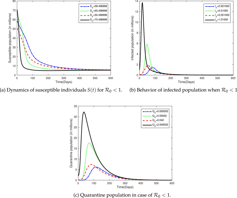
For this set of parameter values, the value of ${\mathcal{R}}_0$ and S ⁰ were calculated 0.2261469439 and 5.343818752, respectively. The simulation was carried out for this set of data as shown in Fig. 6 .

Fig. 6.

The plot shows the dynamics of susceptible, infected and quarantined individuals for different initial population in case of ${\mathcal{R}}_0<1$.

By using the values shown in Table 2, sample simulation were carried out for susceptible population. We have consider four different initial population of susceptible individual, that is, $S_0=58.498998,65.498998,50.498998,$ 70.498998 where the population was considered in million and 58.498998 million is the actual population of the Hubie province. Fig. 6a shows that all of the susceptible population will approach to 5.343818752 irrespective of its initial values whenever ${\mathcal{R}}_0<1$. In the case of ${\mathcal{R}}_0<1,$ each solution curve S(t) almost taking 550 days in order to reach to its equilibrium value $S^0=5.343818752$. It means that if the we wish to eliminate the disease from the community, still it will take almost one and half year. Further, the figures shows that the disease will effect a major portion of the population during the indicated course of outbreak.

The dynamics of infected population in case of ${\mathcal{R}}_0<1$ was plotted in Fig. 6b for initial infected population $I\left(t\right)=0.001000\text{actual},0.01000,0.051000,1.01000$ millions. It is clear from the plot that the if we increase the initially infected people, it will markedly contribute to infected population at initial stages. However, the infection may completely eliminated from the community after 250 days irrespective of the initial infected population if we kept ${\mathcal{R}}_0<1$. It means that if we able to reduce the basic reproduction rate was decreased to less than one, the disease will dies out from the province after more than eight months. In the same way, we plotted Q(t) for different values of Q(0), i.e., 0.000002 actual, 0.00002, 0.042, 2.000002 millions for ${\mathcal{R}}_0<1$ in Fig. 6c. During initial period of the infection, quarantine people may be increased if we increased the initial value of Q(0). However, in long run (almost 400 days) all of the solution curves Q(t) approaches zero irrespective of its initial values. Thus, for elimination of COVID-19 form Hubie it is necessary to keep the value of ${\mathcal{R}}_0<1$. During initial phase of outbreak, more people have close contact history with infected so one must quarantine major portion of the population. However, as the time evolves, the quarantine people will tend to decline and eventually goes to zero. Further, Figs. 6a-6 c verify our theoretical findings that the disease-free equilibrium is locally and globally asymptotically stable if and only if ${\mathcal{R}}_0<1$.

Next, we assumed the real value of Λ, i.e., $\Lambda =0.3805333333$ and use the same values of other parameters as in Table 2 and study the dynamical analysis of the model under discussion numerically. The corresponding values of ${\mathcal{R}}_0$ and endemic equilibrium was calculated as follows:

$${\mathcal{R}}_0=2.261469439,S^{*}=23.62985172,$$

$$I^{*}=1.511070942,Q^{*}=11.19220059.$$ (23)

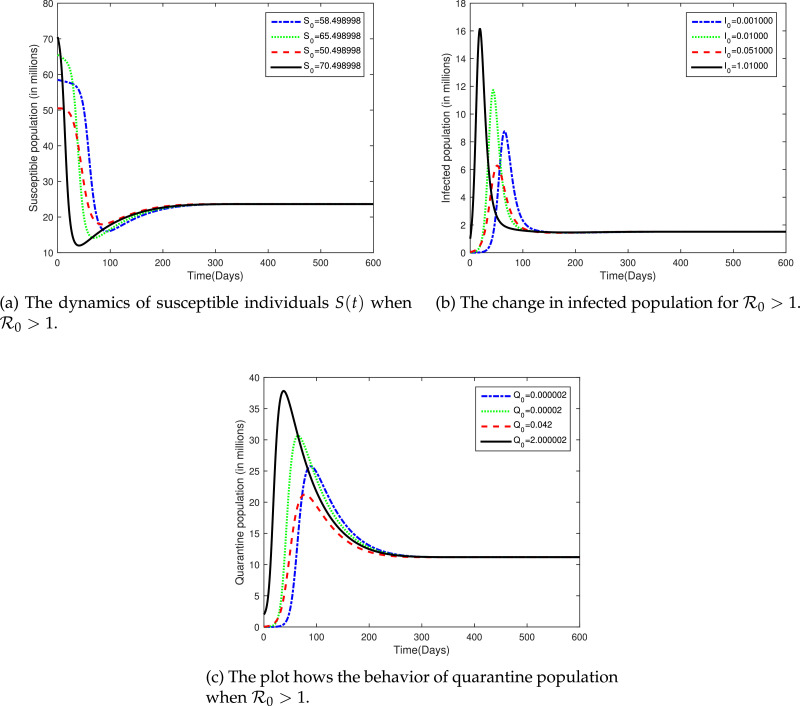
The global analysis of all of the classes were presented in Fig. 7 for ${\mathcal{R}}_0>1$.

Fig. 7.

The plot shows the dynamical behavior of susceptible, infected and quarantine classes for different values of initial population for ${\mathcal{R}}_0>1$.

In Fig. 7a, we have consider again the same initial population of susceptible individual, i.e., 58.498998, 65.498998, 50.498998, 70.498998 millions, however, the value of ${\mathcal{R}}_0$ is now greater than unity. It is clear from the figure, that the susceptible population will tend to decrease/increase during initial 250 days of the infection and afterward it will show no effect. That is, in long run the susceptible population will stabilize itself and will approaches 23.62985172.

Fig. 7 b shows that due to an increase in the initially infected people a sudden increase may be observed later on, i.e., initial 50–80 days. The infection will increase in first 50 days and afterward decreases gradually. However, using the current epidemic status in the province, it is to be noted that the disease will persist in the population. The disease will attain its endemic status during initial 150 days and after that 1.511070942 million infected people will persist in the community if control measures were not implemented properly. In Fig. 7c, we plotted sample simulations of Q(t) for different initial value of the state. All of the curves tend to stabilize itself during initial 300 days. A sudden increase could be observed at early stages and then a gradual decrease in quarantine population irrespective of the initial population. It is clear from the figure that as ${\lim }_{t\to \infty }Q\left(t\right)=11.19220059=Q^{★}$. These figures suggest that the infection will persist in the Hubie province if the current situation remains the same. However, now Chinese data suggest that COVID-19 is well-controlled by Chinese government.

7. Optimal control analysis

One of the very applied and effective analysis to design the control programme for infectious diseases is optimal control theory, see for detail [12], [20], [22], [23], [24], [25], [26], [27], [28], [29], [30]. The optimal control theory will be utilized to design a control mechanism for COVID-19 on the basis of local sensitivity analysis. Here our main purposes are:

• •Reducing vulnerability to COVID-19 by isolating susceptible population and limiting its movement to only non-dangerous zones. This control will be implemented to susceptible population and will be denoted by u ₁(t).
• •Reducing COVID-19 infected people via treatment. Our strategy is to imposed this control on infected people and amount of this control at any time t will be represented by u ₂(t).
• •Most importantly we will maximize the size of the class Q(t) in order to reduce the spread of the disease with minimum cost.

Here it could be noted that it would make sense if the isolation of the vulnerable population but the treatment of infected agents are taken. For this we modify system (1) by incorporating isolation u ₁(t) for S(t) and treatment u ₂(t) for I(t). So from this it is straight forward that model (1) becomes a special case control model if we let $u_1\left(t\right)=0$ (the case of no isolation) and $u_2\left(t\right)=0$ (the case of no treatment). There are various types of representations of the control variables in the corresponding system. Majority of the researchers used $(1-u(t\left)\right)I\left(t\right)$ type of representation (like in [31]), whereas, other use u(t)I(t) (like in [32]) or r ₀ u(t)I(t) (like in [1]) etc. In the present study, the authors used the techniques of [32]. For minimization purpose, we formulate the objective functional of the form

$$\begin{array}{ccc}& & \mathcal{J}(u_1,u_2)=\hfill \\ & & {\int }_0^T[{\xi }_{1}S\left(t\right)+{\xi }_{2}I\left(t\right)-{\xi }_{3}Q\left(t\right)+\frac{1}{2}({\xi }_4{u}_1^2\left(t\right)+{\xi }_5{u}_2^2\left(t\right))]dt,\hfill \end{array}$$ (24)

subject to

$$\begin{array}{cc}\frac{d}{dt}S\left(t\right)\hfill & =\Lambda -\gamma S\left(t\right)I\left(t\right)-d_{0}S\left(t\right)-S\left(t\right)u_1\left(t\right),\hfill \\ \frac{d}{dt}I\left(t\right)\hfill & =\gamma S\left(t\right)I\left(t\right)-(d_0+k+\eta )I\left(t\right)+\sigma Q\left(t\right)-u_2\left(t\right)I\left(t\right),\hfill \\ \frac{d}{dt}Q\left(t\right)\hfill & =\eta I\left(t\right)-(d_0+\mu +\sigma )Q\left(t\right)+S\left(t\right)u_1\left(t\right)+u_2\left(t\right)I\left(t\right),\hfill \end{array}$$ (25)

with

$$S_0>0,I\left(0\right)=I_0\ge 0,Q\left(0\right)=Q_0\ge 0.$$ (26)

In the objective functional (24), ξ ₁, ξ ₂ and ξ ₃ are the weights constants. Moreover ξ ₄ and ξ ₅ are also the positive constants, measures the relative cost on isolation and treatment respectively. Eq. (24) has a clear goal: to decrease the number of people who are at risk as well as infected persons and maximizing the quarantined population. Many researchers assumed that the susceptible population has no concern with the objective functional. However, we believed that more susceptible individual means more people at risk. The longer the time that a vulnerable individual stays in the susceptible state, the longer he or she will be exposed to the disease and it is more likely that individual will be infected. By minimizing vulnerability to the infection ultimately lead towards elimination of the disease from the community. That is why we included the susceptible population in the objective functional. A population can be protected from disease in many ways. For example, the number of susceptible individuals can be reduced through immunizations, the contact rate can be reduced through quarantines or public health campaigns, or the removal rate can be increased through better medical treatment of the sick. In this study, we included quarantine as immunization strategy in the model. It is worthy to notice that quarantine individuals do not participate in the total active population, thus, it should be maximized in any control program. We wish to minimize the objective functional, so a term with negative sign will be ultimately maximized and the same was reflected in our objective functional in case of Q(t). Thus, our objective is to find $(u_1^{*},u_2^{*})$ such that

$$\mathcal{J}(u_1^{*},u_2^{*})=\min \{\mathcal{J}(u_1,u_2),u_1,u_2\in U\},$$ (27)

subject to the control system (25) and (26), where U, the control set is as

$$\begin{array}{ccc}\hfill U:& & =\{(u_1,u_2)|0\le u_1\le l_1,0\le u_2\hfill \\ & & \le l_2,u_1,u_2\text{is}\text{Lebesgue}\text{measurable}\text{on}[0,T]\}.\hfill \end{array}$$ (28)

First we show the existence analysis of such controls.

7.1. Existence

We prove that there is a solution to problem (24)–(26), which exists. So clearly the control functions are Lebesgue measurable and not negative, therefore with nonnegativity of initial data it is very handy to investigate that a solution with the axiom of bounded-ness and positivity exists, for example see for more detail [24], [25], [26].

Let

$$\frac{d\Phi }{dt}=A\Phi +X\left(\Phi \right),$$ (29)

where

$$\begin{array}{cc}\Phi \hfill & =\left(\begin{array}{c}S\left(t\right)\\ I\left(t\right)\\ Q\left(t\right)\end{array}\right),\hfill \\ A\hfill & =\left(\begin{array}{ccc}-d_0-u_2\left(t\right)& 0& 0\\ 0& -(d_0+k+\eta +u_2\left(t\right))& \sigma \\ u_1\left(t\right)& u_2\left(t\right)+\eta & -(d_0+\mu +\sigma )\end{array}\right),\hfill \\ X\left(\Phi \right)\hfill & =\left(\begin{array}{c}\Lambda -\gamma S\left(t\right)I\left(t\right)\\ \gamma S\left(t\right)I\left(t\right)\\ 0\end{array}\right).\hfill \end{array}$$

Clearly Eq. (29) shows that it is a nonlinear equation and the coefficient are bounded. Now we set

$$G\left(\Phi \right)=A\Phi +\psi \left(\Phi \right),$$ (30)

which satisfies

$$\begin{array}{cc}\mid \psi \left({\Phi }_1\right)-\psi \left({\Phi }_2\right)\mid \hfill & \le n_1\mid S_1\left(t\right)-S_2\left(t\right)\mid +n_2\mid I_1\left(t\right)-I_2\left(t\right)\mid \hfill \\ & +n_3\mid Q_1\left(t\right)-Q_2\left(t\right)\mid \hfill \\ & \le N(\mid S_1\left(t\right)-S_2\left(t\right)\mid +\mid I_1\left(t\right)-I_2\left(t\right)\mid \hfill \\ & +\mid Q_1\left(t\right)-Q_2\left(t\right)\mid ,\hfill \end{array}$$ (31)

where $N=\max \left\{(n_1,n_2,n_3)\right\}$ is free of state variables of (1). We also write

$$\mid G\left({\Phi }_1\right)-G\left({\Phi }_2\right)\mid \le M\mid {\Phi }_1-{\Phi }_2\mid ,$$ (32)

where $M=\max \{N,\parallel A\parallel \}<\infty ,$ which implies that G is uniformly Lipschitz continuous. This from the control functions and non-negativity of state variables, it is easy to conclude existence of solution.

We show the optimal values of the control variable minimize the objective function in the following result.

Theorem 4

There exist optimal values of the controls namely $u^{*}=(u_1^{*},u_2^{*})\in U$ which is the solution of the control problem (24) – (26) .

Proof

It is already shown that the control and state functions are not negative. Further, the set U as stated by Eq. (28) that the controls functions are closed as well as convex. Moreover, the bounded-ness of system (25) shows that the necessary compactness holds. It is also to be noted that the state and control functions within objective functional indicated the convexity of objective functional. Hence there exist optimal controls $(u_1^{*},u_2^{*})$. □

7.2. Optimality conditions

To show the characterization of the optimal solution to (24)–(26), we need to define the Lagrangian as well as Hamiltonian for the proposed control problem. Let us symbolize $x=(S,I,Q)$ and $u=(u_1,u_2)$. Then the Lagrangian L is defined by

$$L(x,u)={\xi }_{1}S\left(t\right)+{\xi }_{2}I\left(t\right)-{\xi }_{3}Q\left(t\right)+\frac{1}{2}({\xi }_4{u}_1^2\left(t\right)+{\xi }_5{u}_2^2\left(t\right)),$$

and the associated Hamiltonian function H becomes

$$H(x,u,\lambda )=-L(x,u)+\lambda ·g(x,u),$$

where $\lambda =({\lambda }_1,\dots ,{\lambda }_3)$ and $g(x,u)=(g_1(x,u),\dots ,g_3(x,u))$ with

$$\begin{array}{cc}{g}_1(x,u)\hfill & =\Lambda -\gamma S\left(t\right)I\left(t\right)-d_{0}S\left(t\right)-S\left(t\right)u_1\left(t\right),\hfill \\ g_2(x,u)\hfill & =\gamma S\left(t\right)I\left(t\right)-(d_0+k+\eta )I\left(t\right)+\sigma Q\left(t\right)-u_2\left(t\right)I\left(t\right),\hfill \\ g_3(x,u)\hfill & =\eta I\left(t\right)-(d_0+\mu +\sigma )Q\left(t\right)+S\left(t\right)u_1\left(t\right)+u_2\left(t\right)I\left(t\right).\hfill \end{array}$$

Thus, the Hamiltonian function becomes

$$\begin{array}{ccc}& & H(x,u,\lambda )={\xi }_{1}S\left(t\right)+{\xi }_{2}I\left(t\right)-{\xi }_{3}Q\left(t\right)+\frac{1}{2}({\xi }_4{u}_1^2\left(t\right)+{\xi }_5{u}_2^2\left(t\right))\hfill \\ & & +{\lambda }_1\left(t\right)(\Lambda -\gamma S\left(t\right)I\left(t\right)-d_{0}S\left(t\right)-u_1\left(t\right)S\left(t\right))\hfill \\ & & +{\lambda }_2\left(t\right)(\gamma S\left(t\right)I\left(t\right)-(d_0+k+\eta )I\left(t\right)+\sigma Q\left(t\right)-u_2\left(t\right)I\left(t\right))\hfill \\ & & +{\lambda }_3\left(t\right)(\eta I\left(t\right)-(d_0+\mu +\sigma )Q\left(t\right)+S\left(t\right)u_1\left(t\right)+u_2\left(t\right)I\left(t\right)).\hfill \end{array}$$ (33)

Next, to find the optimal solution, we use the standard Pontryagin’s Maximum Principle [19], [20], if (x*, u*) is an optimal solution for the proposed control problem (24)–(26), then there exists a non-trivial vector function λ such that the Hamiltonian system

$$\{\begin{array}{c}{\displaystyle \frac{d\lambda \left(t\right)}{dt}=-\frac{\partial H}{\partial x}(x^{*}\left(t\right),u^{*}\left(t\right),\lambda \left(t\right)),}\hfill \\ {\displaystyle \frac{\partial H(x^{*}\left(t\right),u^{*}\left(t\right),\lambda \left(t\right))}{\partial u}=0,}\hfill \end{array}$$ (34)

the maximality condition

$$H(x^{*}\left(t\right),u^{*}\left(t\right),\lambda \left(t\right))=\underset{u\in [0,l_1]\times [0,l_2]}{\max }H(x^{*}\left(t\right),u,\lambda \left(t\right)),$$ (35)

and the transversality condition

$$\lambda \left(T\right)=0,$$ (36)

hold.

Theorem 5

Let S*, I*, and Q* be the optimal values of states variables associated to the optimal controls $(u_1^{*},u_2^{*})$ for problem (24) – (26) . Then, there exist adjoint variables λ_i(t), $i=1,2,3,$ satisfying

$$\begin{array}{cc}\frac{d{\lambda }_1\left(t\right)}{t}\hfill & =\gamma I\left(t\right){\lambda }_1\left(t\right)+d_0{\lambda }_1\left(t\right)+u_1\left(t\right){\lambda }_1\left(t\right)-\gamma I\left(t\right){\lambda }_2\left(t\right)\hfill \\ & -u_1\left(t\right){\lambda }_3\left(t\right)-{\xi }_1,\hfill \\ \frac{d{\lambda }_2\left(t\right)}{t}\hfill & =\gamma S\left(t\right)({\lambda }_1\left(t\right)-{\lambda }_2\left(t\right))+(d_0+k+\eta ){\lambda }_2\left(t\right)\hfill \\ & +u_2\left(t\right){\lambda }_2\left(t\right)-(\eta +u_2\left(t\right)){\lambda }_3\left(t\right)-{\xi }_2,\hfill \\ \frac{d{\lambda }_3\left(t\right)}{t}\hfill & =-\sigma {\lambda }_2\left(t\right)+(d_0+\mu +\sigma ){\lambda }_3\left(t\right)+{\xi }_3,\hfill \end{array}$$ (37)

with terminal (transversality) conditions

$${\lambda }_i\left(T\right)=0,i=1,2,3.$$ (38)

Moreover, the optimal control functions $u_1^{*}\left(t\right)$ and $u_2^{*}\left(t\right)$ are represented by

$$u_1^{★}\left(t\right)=\max \{0,\min \{\frac{({\lambda }_1\left(t\right)-{\lambda }_3\left(t\right))S^{★}\left(t\right)}{{\xi }_4},l_1\left\}\right\},$$ (39)

and

$$u_2^{★}\left(t\right)=\max \{0,\min \{\frac{({\lambda }_2\left(t\right)-{\lambda }_3\left(t\right))I^{★}\left(t\right)}{{\xi }_5},l_2\left\}\right\}.$$ (40)

Proof

The adjoint system (37) is calculated from equations (33) with the help of adjoint variables and Pontryagin Principle, while the conditions (38) are the direct consequences of transversality condition as stated by Eq. (36). To find the optimal values for control functions, differentiating H with respect to the control variables and then solving the pair of equations $\frac{\partial H}{\partial u_1}=0$ and $\frac{\partial H}{\partial u_2}=0$. Keeping in mind the upper and lower bounds of the control measures we can present the characterization of the control defined in (39)–(40) and hence proved. □

We founded that the optimal values of states and controls by solving analytically the optimal system, which includes the states (25) and the adjoint Eq. (37), boundary conditions (26) and (38), along with the characterization of optimal control variables $(u_1^{*},u_2^{*})$ in the form of (39) and (40).

7.3. Simulation on control strategies of COVID-19

In order to obtain the numerical solution for the control problem, we will use Runge-Kutta procedure of order four. More precisely, we descritize the original model (1), the control model (25), the adjoint system (37) and will coded the same in MATLAB along with subsidiary conditions (26), (38) and the characterization of the control (39)-(40). The parameter values used for simulating the control and uncontrolled problem is depicted in Table 3 .

Table 3.

Values and sources of parameter used in numerical simulation.

Parameter	Value	Source
Λ	0.3805333333	Calculated [3]
γ	0.00594474	Estimated
d0	0.007121000000	[3]
η	0.144211141	Estimated
ν	0.007121000000	[3]
σ	0.0052281	Estimated
k	0.027864676	Estimated
ξ1	30	Estimated
ξ2	400	Estimated
ξ3	0.005	Estimated
ξ4	2,000,000	Fitted
ξ5	500	Estimated

The simulation for the control and without control problems were carried out and a comparison was presented among real data, without control and with control curves in Fig. 8 for all classes.

Fig. 8.

Dynamics of real data, without control and with control problem.

Fig. 8 a shows the dynamics of susceptible population in three different perspective. If we compare the uncontrolled curve with real data, we reach to the conclusion that our model best fit the realistic scenario. Further, it is clear that without implication of the control strategies, more people will be vulnerable to the disease and eventually a particular portion of the population will be prone to the disease at all the time. However, if we imposed the control strategies upon the susceptible people, the population will tend to decline and after 100 days there will be no susceptible individual in the community.

Again, Fig. 8b shows that our proposed model best explain the dynamics of COVID-19 in the Hubie province. Figure suggest that if we ignore the control policy, the infection will tend to grow and the decrease and eventually persist constantly in the Hubie province for long run. However, after 100 days there will be no infection if one impose the control strategies in true spirit. Similarly, the usefulness of the proposed model and the best output of the control upon quarantine population could be observed in Fig. 8c. Thus, we can say that the model under consideration is correct up to the mark for explaining the dynamics of COVID-19 in Hubie province and to eliminate the disease, it is most beneficial and effective to adopt the same control strategies as outlined in the current study.

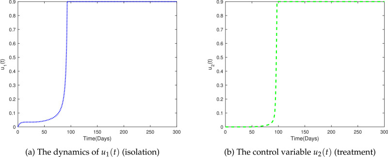
Figs. 9 a and 9 b shows the dynamics of the control variables u ₁(t) and u ₂(t). During initial phase of the control policy (up to 60 days), the control u ₁(t) have very low effect upon the susceptible people, afterward, the control tend to increase very fast and finally reach to its maximum value. Similarly, the control u ₂(t) is silent till initial 70 days and then start working with maximum returns.

Fig. 9.

The dynamics of control variables.

8. Discussion

Keeping in view the ongoing disastrous spread of the novel coronavirus (COVID-19) across the globe, we have proposed a robust mathematical model that is able of assisting the health regulatory authorities in adopting important safety measures and management strategies for controlling such spreads. In order to test the validity and accuracy of the proposed model, in this paper, we have considered Hubei Province of the People’s Republic of China, and is part of the Central China region. We have conducted a detailed analysis of our model, and applied it to study the Wuhan epidemic using publicly reported data. Parameters in the basic reproduction number ${\mathcal{R}}_0$ of this model comes from three compartments; i.e., from the quarantine individuals, the infected individuals, and susceptible individuals. We have established the global asymptotic stability of the disease-free equilibrium when ${\mathcal{R}}_0<1,$ and the global asymptotic stability of the endemic equilibrium when ${\mathcal{R}}_0>1$. Our numerical simulation results demonstrate the application of our model to the COVID-19 outbreak in Wuhan. Our model best fit the reported data very well. Through data fitting, we obtain an estimate of basic reproduction number, ${\mathcal{R}}_0=2.261469439$. Our model predicts the appearance of an epidemic peak, after which the infection level would decrease and approach an endemic state in the long run. We also find that if we use constant transmission rates instead, the model would predict a much higher and unrealistic epidemic peak. This is caused by the fixed transmission rates that do not reflect the impact of on-going disease control measures. It is an indication that using epidemiologically and environmentally dependent transmission rates can potentially generate more practical simulation results.

At present, many aspects regarding the pathology, ecology and epidemiology of the novel coronavirus remain unknown [30], which add challenges to mathematical modeling. Particularly, in our current model, we have employed a bilinear incidence rate based on the law of mass action to represent the human-to-human transmission route. Though, a saturation based incidence rate might better characterize the environmental pathogen, and we hope to investigate it in our future modeling efforts. Given the current development of COVID-19, it is widely speculated that this disease would persist in the human world and become endemic. Our mathematical analysis and numerical simulation results support this speculation. The findings in this study imply that we should be prepare our self to fight the coronavirus infection for a much longer term than that of the current epidemic wave, in order to reduce the endemic burden and potentially eradicate the disease eventually. Among other intervention strategies, new vaccines for the novel coronavirus, which are currently in research and development, could play an important role in achieving that goal. Further, our study strongly support the fact if we imposed the two indicated control measures, we can easily eliminate the COVID-19 in almost 100 days from Wuhan. We emphasize that our data fitting is based on the reported confirmed cases in Wuhan from January 21, to March 2, in 2020. These confirmed cases were determined by the method of nucleic acid testing kits. On February 12, 2020, the national health commission in China started including cases confirmed by another method; i.e, clinical diagnosis, which refers to using CT imaging scans to diagnose patients. This change of criteria led to a surge of confirmed cases on February 12, (with an increase of about 14,000 new cases for Wuhan in a single day). We plan to address the new development of the outbreak data in another piece of work in the near future. We also plan to expand our modeling efforts to the province and country levels beyond the epicenter, the city of Wuhan, and study the spread of the novel coronavirus in larger spatial scales.

In a nutshell, we can say that understanding the dynamics of a fast-moving disease (like COVID-19) in the early stages of a pandemic is indeed a challenging task for the health official and policy makers. A single model is not appropriate, and long-term predictions of such models are likely to be futile. Perhaps, one can use model to short-term data which will enables us to comprehend deeply the existing data as well as to make predictions when data is unavailable. For this purpose, fast-moving models should be developed and analyzed for better understanding of such diseases. The strategy of short-term data fits will definitely help us to control the spread of COVID-19 at earliest. As infectious disease will be always with us, thus, the results of a model could be applied to any next disease if not working for the current situation.

9. Conclusions

In this article, we have established a model for the transmission dynamic of novel CoVID-2019 by taking into account the classification of different phases of its spread in population. First, we studied the statistics of novel CoVID-2019 in Hubie, China and then we combined different characteristics of the disease and formulated a mathematical model which describe the dynamics of the infection. Further, we presented different mathematical analysis on the proposed model including boundedness, biological feasibility, positivity and existence of equilibria of the proposed model. For analysis purpose, initially we obtained the basic reproduction number and then derived all the disease-free and endemic equilibrium of the model. The local and global stability of the disease-free equilibrium was carried out by using the linearization and Lyapnove functional theory, respectively. The DFE is globally asymptotically stable if ${\mathcal{R}}_0<1$. Similarly, it is shown that the endemic equilibrium is locally, as well as globally asymptotically stable whenever ${\mathcal{R}}_0>1$. The value of ${\mathcal{R}}_0$ was calculated for the COVID-19 at Hubie and it was founded that the disease will persist for long term if not properly addressed. Finally, the numerical simulation and sensitivity analysis were presented to show the feasibility of the proposed model and effectiveness of the control strategies.

Declaration of Competing Interest

The authors declare that they have no known competing financial interests or personal relationships that could have appeared to influence the work reported in this paper.

References

- 1.Maclachlan, James N., Edward J. Academic press; 2010. Fenner’s veterinary virology. [Google Scholar]
- 2.Ji W., Wang W., Zhao X., Zai J., Li X. Crossspecies transmission of the newly identified coronavirus 2019ncov. J Med Virol. 2020;92(4):433–440. doi: 10.1002/jmv.25682. [DOI] [PMC free article] [PubMed] [Google Scholar]
- 3.Organization W.H. Switzerland, 24 January 2020. No. WHO/HEO/R&D Blueprint (nCoV)/2020.1. World Health Organization; 2020. WHO R&D Blueprint: informal consultation on prioritization of candidate therapeutic agents for use in novel coronavirus 2019 infection, geneva. [Google Scholar]
- 4.Lau, Susanna K.P., Fan R.Y.Y., Luk H.K.H., Zhu L., Fung J., Li K.S.M., Wong E.Y.M. Replication of MERS and SARS coronaviruses in bat cells offers insights to their ancestral origins. Emerg Microbe Infect. 2018;7(1):1–11. doi: 10.1038/s41426-018-0208-9. [DOI] [PMC free article] [PubMed] [Google Scholar]
- 5.Chan, Fuk-Woo J., Yuan S., Kok K.-H., To K.K.-W., Chu H., Yang J., Xing F. A familial cluster of pneumonia associated with the 2019 novel coronavirus indicating person-to-person transmission: a study of a family cluster. Lancet. 2020;395(10223):514–523. doi: 10.1016/S0140-6736(20)30154-9. [DOI] [PMC free article] [PubMed] [Google Scholar]
- 6.Huang, Chaolin, Wang Y., Li X., Ren L., Zhao J., Hu Y., Zhang L. Clinical features of patients infected with 2019 novel coronavirus in wuhan, china. Lancet. 2020;395(10223):497–506. doi: 10.1016/S0140-6736(20)30183-5. [DOI] [PMC free article] [PubMed] [Google Scholar]
- 7.Tavakoli, Ahmad, Vahdat K., Keshavarz M. Novel coronavirus disease 2019 (COVID-19): an emerging infectious disease in the 21st century. ISMJ. 2020;22(6):432–450. [Google Scholar]
- 8.Huang, Chaolin, Wang Y., Li X., Ren L., Zhao J., Hu Y., Zhang L. Clinical features of patients infected with 2019 novel coronavirus in wuhan, china. Lancet. 2020;395(10223):497–506. doi: 10.1016/S0140-6736(20)30183-5. [DOI] [PMC free article] [PubMed] [Google Scholar]
- 9.Chen, Nanshan, Zhou M., Dong X., Qu J., Gong F., Han Y., Qiu Y. Epidemiological and clinical characteristics of 99 cases of 2019 novel coronavirus pneumonia in wuhan, china: a descriptive study. Lancet. 2020;395(10223):507–513. doi: 10.1016/S0140-6736(20)30211-7. [DOI] [PMC free article] [PubMed] [Google Scholar]
- 10.Deng, Sheng-Qun, Peng H.-J., 9. Characteristics of and public health responses to the coronavirus disease 2019 outbreak in china. J Clin Med. 2020;(2):575. doi: 10.3390/jcm9020575. [DOI] [PMC free article] [PubMed] [Google Scholar]
- 11.Mission . Report of the WHO-china joint mission on coronavirus disease 2019 (COVID-19). Geneva 2020. 2020. WHO-China joint. [Google Scholar]
- 12.Khan T., Zaman G., Chohan M.I. The transmission dynamic and optimal control of acute and chronic hepatitis b. J Biol Dyn. 2017;11:172–189. doi: 10.1080/17513758.2016.1256441. [DOI] [PubMed] [Google Scholar]
- 13.LaSalle, Joseph P. The stability of dynamical systems. Siam. 1976;25 [Google Scholar]
- 14.van den Driessche P., Watmough J. Mathematical epidemiology, Lecture Notes in Math. vol. 1945. Springer; Berlin: 2008. Further notes on the basic reproduction number; pp. 159–178. [Google Scholar]
- 15.Atangana, Abdon Modelling the spread of COVID-19 with new fractal-fractional operators: can the lockdown save mankind before vaccination? Chaos Solitons Fractals. 2020;136:109860. doi: 10.1016/j.chaos.2020.109860. [DOI] [PMC free article] [PubMed] [Google Scholar]
- 16.Khan, Altaf M., Atangana A. Modeling the dynamics of novel coronavirus (COVID-19) with fractional derivative. Alexandria Eng J. 2020 [Google Scholar]
- 17.Mann J., Roberts M. Modelling the epidemiology of hepatitisb in newzealand. J Theor Biol. 2011;269:266–272. doi: 10.1016/j.jtbi.2010.10.028. [DOI] [PubMed] [Google Scholar]
- 18.Culshaw R.V., Ruan S., Spiteri R.J. Optimal HIV treatment by maximising immune response. J Math Biol. 2004;48:545–562. doi: 10.1007/s00285-003-0245-3. [DOI] [PubMed] [Google Scholar]
- 19.Kamien, Morton I., Nancy Lou S. Dynamic optimization: the calculus of variations and optimal control in economics and management. Cour Corp. 2012 [Google Scholar]
- 20.Zaman G., Kang Y.H., Jung I.H. Optimal treatment of an SIR epidemic model with time delay. BioSystems. 2009;98:43–50. doi: 10.1016/j.biosystems.2009.05.006. [DOI] [PubMed] [Google Scholar]
- 21.Dahlard J., Lukes L. Academic Press, Inc. [Harcourt Brace Jovanovich, Publishers]; London-New York: 1982. Differential equations, mathematics in science and engineering, vol. 162. [Google Scholar]
- 22.Din, Anwarud, Li Y., Liu Q. Viral dynamics and control of hepatitis b virus (HBV) using an epidemic model. Alexand Eng J. 2020;59(2):667–679. [Google Scholar]
- 23.Khan T., Ullah Z., Ali N., Zaman G. Modeling and control of the hepatitis b virus spreading using an epidemic model. Chaos Solit Fract. 2019;124:1–9. [Google Scholar]
- 24.Khan A., Zaman G. Optimal control strategy of SEIR endemic model with continuous age-structure in the exposed and infectious classes. Optim Control Appl Meth. 2018;39:1716–1727. [Google Scholar]
- 25.Li X., Yong J. Optimal control theory for infinite dimensional systems. Birkhuser: Boston. 1995 [Google Scholar]
- 26.Lukes D.L. Mathematics in science and engineering. Academic Press; New York: 1982. Differential equations: classical to controlled. [Google Scholar]
- 27.Anderson R.M., May R.M. Oxford University Press; Oxford: 1992. Infectious diseases of humans: dynamics and control. [Google Scholar]
- 28.Thater M., Chudej K., Pesch H.J. Optimal vaccination strategies for an SEIR model of infectious diseases with logistic growth. Math Biosci Eng. 2017;15(2):485–505. doi: 10.3934/mbe.2018022. [DOI] [PubMed] [Google Scholar]
- 29.Frew, Emma . Oxford University Press; 2010. Applied methods of cost-benefit analysis in health care. Vol. volume 4. [Google Scholar]
- 30.Tien J.H., Earn D.J.D. Multiple transmission pathways and disease dynamics in a waterborne pathogen model. Bull Math Biol. 2010;72:1506–1533. doi: 10.1007/s11538-010-9507-6. [DOI] [PubMed] [Google Scholar]
- 31.Jan R., Khan M.A., Gmez-Aguilar J.F. Asymptomatic carriers in transmission dynamics of dengue with control interventions. Optim Control Appl Meth. 2019:1–18. doi: 10.1002/oca.2551. [DOI] [Google Scholar]
- 32.Agusto F.B., Khan M.A. Optimal control strategies for dengue transmission in Pakistan. Math Biosci. 2018;305:102–121. doi: 10.1016/j.mbs.2018.09.007. [DOI] [PubMed] [Google Scholar]