Fluorescence imaging and Raman spectroscopy applied for the accurate diagnosis of breast cancer with deep learning algorithms

Abstract

Deep learning is usually combined with a single detection technique in the field of disease diagnosis. This study focused on simultaneously combining deep learning with multiple detection technologies, fluorescence imaging and Raman spectroscopy, for breast cancer diagnosis. A number of fluorescence images and Raman spectra were collected from breast tissue sections of 14 patients. Pseudo-color enhancement algorithm and a convolutional neural network were applied to the fluorescence image processing, so that the discriminant accuracy of test sets, 88.61%, was obtained. Two different BP-neural networks were applied to the Raman spectra that mainly comprised collagen and lipid, so that the discriminant accuracy of 95.33% and 98.67% of test sets were gotten, respectively. Then the discriminant results of fluorescence images and Raman spectra were counted and arranged into a characteristic variable matrix to predict the breast tissue samples with partial least squares (PLS) algorithm. As a result, the predictions of all samples are correct, with minor error of predictive value. This study proves that deep learning algorithms can be applied into multiple diagnostic optics/spectroscopy techniques simultaneously to improve the accuracy in disease diagnosis.

1. Introduction

Breast cancer is one of the most common malignant tumors. Therefore, it is of great significance to achieve accurate diagnosis and treatment of this disease. Common diagnostic methods include pre-operative, intra-operative and post-operative diagnosis. As a preoperative diagnostic technique, X-ray CT is widely used in clinical diagnosis. But it is not suitable for regular screening with its toxicity and insensitive to high-density breast tissue [1]. Magnetic resonance imaging (MRI) is non-toxic, whereas it is expensive and time-consuming [2]. Intra-operative frozen breast cancer diagnosis technique is one of the intra-operative diagnostic methods. However, its accuracy may be affected by age, tumor size and patients’ mammography calcified point situation [3]. As for postoperative diagnosis, the significance of pathological evaluation and morphological assessment in the field of diagnosis and treatment have become crucial since they provide important prognostic information [4,5]. However, the diagnosis of breast cancer mostly depends on experienced experts, the diagnosis process is not only time-consuming but also influenced by subjective factors. Thus, an automatic diagnosis technique for accurate and objective diagnosis of breast cancer in a short time is still necessary [6].

Deep learning algorithm is a popular machine learning algorithm that analyzes intricate structure in big data sets by using the backpropagation algorithm [7]. It is expert in translating biomedical big data into valuable information rapidly and insightfully [8]. Since its great potential in rapid and accurate diagnosis of disease, deep learning algorithm has been applied to different diagnostic techniques (such as histopathological imaging [9], biomarker score [10], and photoacoustic tomography imaging [6]) to investigate the possibility of automatic diagnosis of breast cancer. But these diagnostic techniques are often complex, sample-contaminating and time-consuming. Hence some rapid and label-free diagnostic techniques such as fluorescence imaging and Raman spectroscopy will have greater potential.

Fluorescence imaging is a molecular imaging technique that reflects the composition information of samples. It is non-toxic, rapid and widely used in biological sample detection [11]. As a potential cancer diagnostic tool [12], Raman spectroscopy is a molecular analytical technique based on the inelastic scattering of photons by molecular bond vibrations, which is nondestructive and unaffected by water. Fluorescence imaging and Raman spectroscopy have been used in breast cancer research in some previous studies. Mahadevan-Jansen's group used Raman spectroscopy to evaluate HER2 amplification status and acquired drug resistance in breast cancer cells [13]. They further explored the feasibility of Raman spectral markers in assessing metastatic bone in breast cancer [14]. Notingher's group combined Raman spectroscopy with fluorescence imaging for tissue detection [15,16] to achieve a rapid and objective intra-operative assessment of breast cancer during tissue-conserving surgery [17]. Puppels's group combined Raman spectroscopy with principal components analysis and K-means cluster analysis to achieve identification of different cellular compounds within the epithelial layer of breast tumors [18]. These studies indicate the potential of Raman spectroscopy combined with fluorescence imaging in breast cancer research.

Deep learning combined with fluorescence imaging had been used to detect subtle changes in nuclear morphometrics at single-cell resolution [19], as well as to classify compounds in chemical mechanisms of action [20]. A one-dimensional convolution neural network and a Raman spectra database were established and combined together to realize multi-identification blood species [21]. These studies show the potential of deep learning combined with either fluorescence imaging or Raman spectroscopy in detection of biological information. However, deep learning algorithm was usually used to combine with a single diagnostic technique. To combine deep learning algorithms to both fluorescence imaging and Raman spectroscopy simultaneously with PLS will be proposed as a promising way to improve the diagnostic accuracy of breast cancer for the first time.

2. Materials and method

2.1. Sample preparation

The breast tissues of 14 patients were harvested from Jiangsu cancer hospital, which was approved by the institutional review committees with informed consent. The specimens were processed in clinic and segmented into cancerous, paracancerous, and normal tissue samples in size of approximate 1 cm, respectively. Paracancerous samples were not used because it might contain both cancerous and normal tissues. The patients were marked as S1-S14 (each of S1-S9 contained both a cancerous and a normal samples; each of S10-S14 only had a cancerous sample). The number of cancerous and normal samples was 14 and 9, respectively.

After the samples were washed in saline and frozen in saline with liquid nitrogen, they were cut into a number of sections with thickness of 15-µm (for clear microscope view) and 150-µm (for strong Raman scattering) by using cryostat (Leica CM 1950, Germany). The sections were picked up by slides for fluorescence imaging and Raman spectral acquisition after air drying.

2.2. Convolutional neural network applied to fluorescence images

Auto-fluorescence images were acquired from 15-µm thick sections. The acquisition area should be close to the center of the sections to avoid possible paracancerous tissue at the edge of the sections. All auto-fluorescence images were collected by using epi-fluorescence microscope (BM2100POL, Nanjing Madison Instrument Co., Ltd). The light emitted from a mercury lamp passed through a excitation filter (BP460-495 nm), then was reflected by a dichroic mirror (DM505 nm) and focused onto the sample through a objective lens (20x). The auto-fluorescence of the sample passed through the dichroic mirror and a barrier filter (BA520 nm), then was collected by a 24-bit CCD (DC6000, Nanjing Madison Instrument Co., Ltd). The field of view was 1 mm. In the process of fluorescence images acquisition, the parameter settings of the acquisition software (ScopeImage 9.0) remained unchanged.

Total 120 fluorescence images were collected from each sample. Then the pseudo-color enhancement was performed on the fluorescence images. The detailed steps of pseudo-color enhancement processing are described as follow.

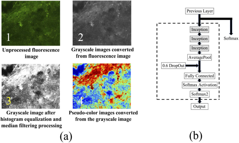
Firstly, the original fluorescence images were converted into grayscale images. Secondly, a histogram equalization algorithm was used to expand the contrast and grayscale range of the grayscale images. Thirdly, a median filtering algorithm was performed on the grayscale images to reduce the noise generated during histogram equalization process. Finally, a density segmentation coding algorithm [22] was used to convert the grayscale images into pseudo-color images.

The pseudo-color images of S9 and S14 were selected as test sets (including 1 normal and 2 cancerous samples, 360 images in total), which was used to evaluate the generalization ability of the neural network. For each remaining sample, 100 of the 120 pseudo-color images were randomly selected as training sets, and the others were used as validation sets.

It is necessary to perform data augmentation on the training sets to extend the amount of it and reduce the risk of over-fitting [23]. Horizontal, vertical, diagonal flipping and rotation at different angles were done to each pseudo-color image of training sets. 1% Gaussian noise was also added to the pseudo-color images to enhance the robustness of the neural network. After that the amount of training sets increased by 10 times to be a total of twenty thousand.

A classical convolutional neural network called GoogLeNet was applied to the pseudo-color images through transfer learning method [6]. Training and discrimination process were completed by MATLAB software programming. The hyperparameters of the training process were continuously adjusted according to the training results.

Receiver operating characteristic (ROC) curve was used to evaluate the performance of the trained neural network model [24]. When doing prediction, the predictive values of the test set were arranged from large to small. In turn, each predictive value was set as threshold, and the corresponding true-positive rate (TPR) and false-positive rate (FPR) of test set were calculated, so that multiple sets of TPR and FPR were obtained. The sets of FPR (as abscissa) and TPR (as ordinate) were plotted in figure to be ROC curve. Then the area-under-curve (AUC) of the ROC curve was calculated. If the value of AUC was greater than 0.9, it indicated that the neural network model has good performance.

2.3. BP-neural networks applied to Raman spectra

A home-made near-infrared micro Raman spectrometer was used in this study. The schematic diagram of its excitation and collection light paths is shown in Fig. 1.

Fig. 1.

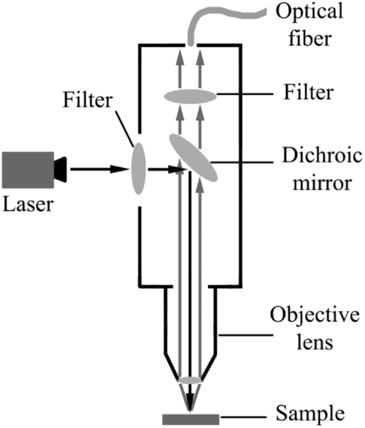
The schematic diagram of excitation and collection light paths in home-made micro Raman spectrometer.

An incident light from 785-nm laser (IPS, USA) with power of 100 mw entered into microscope system after passing through a filter, then was reflected by dichroic mirror and focused onto the sample (60 mW) through the objective lens. The Raman scattering light was collected by the objective lens, passed through dichroic mirror and filter, and then entered into the optical fiber. The Raman scattering light finally passed through the optical fiber and was detected in a dispersion system. The optical fiber had a core diameter of 400-µm and a numerical aperture of 0.22. The Raman scattering light was collected in a circular area of 20-µm diameter on the surface of the sample. A 16-bit cooling type CCD (Andor, iVac 316) with an operating temperature of -60 °C was installed in the dispersion system. The range of spectral collection was from 500 to 2000cm^-1 with spectral resolution of 3 cm^-1 [25]. Exposure time was set as 30s for each measurement with operating software of Andor Solis.

After 60 Raman spectra were collected from each sample, the fluorescence background was corrected by using the automated background subtraction algorithm developed by Zeng and colleagues [26]. Then data augmentation was performed on the Raman spectra. The spectra were translated left or right by one wave number, or multiplied by different ratios (total sum of ratios was 100%) and then added up. 1% Gaussian noise was also added to the spectra to improve the robustness of the networks. After that the spectral number of each sample was expanded to 100.

The spectra of S9 and S14 were selected as test sets (containing 300 spectra). For each remaining sample, 90 spectra were randomly selected as training sets, and the others were used as validation sets.

BP-neural networks were applied into the Raman spectral analysis. The training and discrimination process were completed by the neural network toolbox in MATLAB software. The hyperparameters of the training process were continuously adjusted according to the training results, which was similar to the training process of googLeNet. ROC curve and AUC were also used to evaluate the performance of the trained neural network models of Raman spectra.

2.4. PLS applied to samples prediction

All the fluorescence images and Raman spectra were discriminated by the trained neural network models, respectively. For each neural network model, the number of data discriminated as positive and negative was counted. Then the true-positive rate, true-negative rate (TNR), false-positive rate and false-negative rate (FNR) were calculated on this basis. The calculated results of each neural network model were merged into a characteristic variables matrix as the input of PLS model. The training and prediction of PLS model were completed by MATLAB programming. Specifically, normal and cancerous samples were labeled as 1 and 2, respectively. The coefficients and a constant term of a PLS regression equation were calculated from the characteristic variable matrix of the training sets. Then the characteristic variables matrix of test sets was imported into the PLS regression equation to obtain the predictive value. The threshold was set as 1.5, and the prediction results of the samples were determined by comparing the predictive value with the threshold. Leave-one-out cross validation (LOOCV) was used to evaluate the stability of the PLS model. In turn, one sample was selected as test set, the remaining samples were used as training sets to achieve PLS model training and prediction. In this way, the stability of the PLS model constructed on the total samples can be fully evaluated [27].

3. Results

3.1. Results of GoogLeNet with fluorescence images

Figure 2 shows the steps and results of the pseudo-color enhancement (Fig. 2(a)), and the modified parts of the GoogLeNet (Fig. 2(b)). Compared with the original fluorescence images, the pseudo-color images have higher contrast and richer color information, which confirms that performing pseudo-color enhancement on the fluorescence images is effective.

Fig. 2.

(a) The steps and results of the pseudo-color enhancement and (b) the modified parts of the GoogLeNet (contained in the dotted line).

In transfer learning process of GoogLeNet, it is necessary to control the number of parameters participating in training to avoid over-fitting. After a series of tests, the last 3 inception modules and the subsequent network layers of GoogLeNet are selected and modified for training. To further reduce the risk of over-fitting, a dropout layer with a probability of 0.6 is added between average-pool layer and fully-connected layer. The modified parts of GoogLeNet are shown in the dotted line in Fig. 2(b).

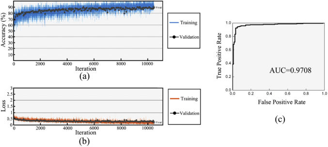
Figure 3 shows the training process and results of the GoogLeNet. When the discriminant accuracy curves of training sets and validation sets show a separation trend (Fig. 3(a)), the training process is stopped to avoid over-fitting. The total number of iterations was 10451. Figure 3(b) shows the loss function curve of training sets and validation sets. Both curves show downward trend, indicating that the training process is effective. Figure 3(c) shows the ROC curve of the test sets. The AUC of the ROC curve was calculated as 0.9708, which confirms the satisfied discriminant ability of the trained GoogLeNet.

Fig. 3.

(a) Discriminant accuracy curves of the training sets (blue curve) and validation sets (black scatter) in training process. (b) loss function curves of the training sets (red curve) and validation sets (black scatter) in training process. (c) The receiver operating characteristic curve of the test sets.

Table 1 shows the discriminant results of fluorescence images by using the trained GoogLeNet. The discriminant accuracy of training sets, validation sets and test sets are relatively close to each other, which further confirms low risk of over-fitting and excellent generalization ability of the trained GoogLeNet.

Table 1. The discriminant results of fluorescence images by using the trained GoogLeNet.

	Sample size	Correct discrimination	Wrong discrimination	Accuracy
Training sets	20000	18003	1997	90.02%
Validation sets	400	358	42	89.5%
Test sets	360	319	41	88.61%

3.2. Results of Raman spectra with bp-neural networks

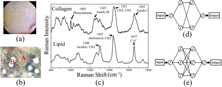
It is found that there are many globose structures that distribute in the extracellular matrix (ECM) in 150-µm thick sections under visible light, as shown in Fig. 4(a) & 4(b). Thus, a number of spectra were collected from the ECM and the globose structures for test. The average spectra of them are calculated and the corresponding characteristic peaks are compared in Fig. 4(c). It is proved that the Raman spectra collected from the ECM and the globose structures are mainly contributed by collagen (type I collagen) and lipid (triglyceride) in breast tissue, respectively [28–31]. Therefore, two BP-neural networks with different structures are constructed for collagen (Fig. 4(d)) and lipid (Fig. 4(e)) spectra.

Fig. 4.

Visible light photo of breast tissue section (150-µm thickness) under (a) 5x and (b) 20x objective lens. The positions marked as A and B in (b) represent the extracellular matrix and the globose structures in the section, respectively. (c) Average spectra of collagen and lipid collected from the ECM and the globose structures, respectively. (d) Schematic diagrams of the structure of BP-neural networks for collagen and (e) lipid.

In the process of spectra acquisition and data augmentation, the spectral amount of collagen is same as that of lipid. The training and discrimination process of collagen and lipid spectra are performed separately.

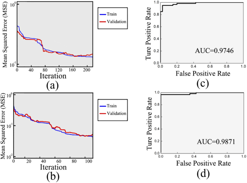
Figure 5 shows the training process and results of the BP-neural networks. Mean squared error (MSE) curves are used to evaluate the training process of BP-neural networks. In Fig. 5(a) & 5(b), all curves show downward trends, suggesting that the training process is effective. When the MSE curve of validation sets shows 10 consecutive upward trends, the training process is stopped to avoid over-fitting. Therefore, the total number of iterations of collagen and lipid spectra was 216 and 105, respectively. The ROC curves of collagen and lipid are obtained and drawn in Fig. 5(c) & 5(d). Then AUC of the ROC curves of collagen and lipid are calculated as 0.9746 and 0.9871, respectively, suggesting the satisfied discriminant ability of the trained BP-neural networks.

Fig. 5.

Mean squared error curves of (a) collagen and (b) lipid. The two curves in either graph correspond to training sets (blue curve) and validation sets (red curve), respectively. Receiver operating characteristic curve of (c) collagen and (d) lipid.

Table 2 shows the discriminant results of Raman spectra of collagen and lipid by using the trained BP-neural networks. Whether collagen or lipid, the discriminant accuracy of validation sets and test sets are high and relatively close to each other, which confirms low risk of over-fitting and excellent generalization ability of the trained BP-neural networks.

Table 2. The discriminant results of Raman spectra by using the trained BP-neural networks.

Component		Sample size	Correct discrimination	Wrong discrimination	Accuracy
Collagen	Training sets	900	892	8	99.11%
	Validation sets	100	97	3	97%
	Test sets	150	143	7	95.33%
Lipid	Training sets	900	890	10	98.89%
	Validation sets	100	100	0	100%
	Test sets	150	148	2	98.67%

In some cases, the collected spectra would be the mixture of collagen and lipid [13-18], so that a new corresponding neural network model must be built based on the mixed spectra to replace the neural network model of either collagen or lipid spectra.

3.3. Results of PLS prediction

Figure 6 shows the LOOCV results of 23 training and prediction processes of the PLS model. A dotted line means the threshold of 1.5. In general, whether the prediction result is correct or not is judged by comparing the predictive value with the threshold. It can be concluded from Fig. 6 that the prediction results of all samples are correct with minor error, which indicates excellent stability and high predictive accuracy of the PLS model.

Fig. 6.

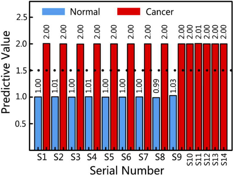
Predictive value of the breast samples with the PLS model. The dashed line represents the threshold of 1.5.

Table 3 is the prediction results of the PLS model based on the results of the neural network models above. The PLS prediction achieved 100% accuracy for all samples, which are better than that of sole neural network model.

Table 3. The prediction results of all samples by using PLS model.

Type of samples	Sample size	Correct discrimination	Wrong discrimination	Accuracy
normal	9	9	0	100%
cancerous	14	14	0	100%

4. Discussion

In the training process of the neural networks, a key issue is to reduce the risk of over-fitting. Once over-fitting occurred, the prediction and generalization ability of the neural networks would be affected seriously. Therefore, several methods as below are tried to reduce the risk of over-fitting in the training process.

The first one is to adjust the number of parameters of neural network participating in training. GoogLeNet is mainly composed of inception modules and contains a large number of parameters [32,33]. Therefore, a flexible training method, transfer learning, was applied to train a small part of the GoogLeNet [34]. Since Raman spectra are composed of one-dimensional variables, the application of the BP-neural networks of Raman spectra is suitable and efficient [35]. In the training process of BP neural networks, the number of parameters is controlled by adjusting the number of layers and nodes.

Second, increasing the amount of training data is effective to reduce the risk of over-fitting. Thus, it is necessary to perform data augmentation on the original data. Data augmentation of Raman spectra has been reported by Zhao's group [36]. And they further investigated the effect of noise on the neural network, showing that the performance of neural network model is scarcely affected by low-noise in spectral data augmentation. The Zhao's work and the results in this study indicate that the data augmentation of Raman spectra supports extending the amount of spectra and has little effect on the accuracy of neural network model.

Third, other method such as adding the dropout layer to the convolutional neural network is also helpful. Finally, the training process is stopped when the discriminant accuracy of validation sets is optimal. As a result, both the validation sets and the test sets of fluorescence images and Raman spectra have high discriminant accuracy, which confirms that the methods above are effective in reducing the risk of over-fitting.

Since no fluorescent dye is used, the brightness and contrast of the auto-fluorescence images obtained from breast tissue are low, and the color information is not rich. In this case, histogram equalization is introduced into fluorescence image processing to enhance textural information. Pseudo-color enhancement processing based on density segmentation coding algorithm further enhances the textural information and enriches the color information of fluorescence images. It was reported that the collagen accounts for up to 30% of breast tissues, which is a source of auto-fluorescence [37–39]. Furthermore, FAD and NADH are also common fluorophores [40,41] and contribute to the auto-fluorescence of breast tissues [40]. Therefore, fluorescence images may reflect the distribution and concentration of collagen, NADH and FAD in breast tissues. In addition, compared with normal breast tissues, the fluorescence of collagen in cancer tissues is reduced, which may be due to the reducing of quantum yield of collagen [42]. The reasons above make fluorescence imaging become an efficient diagnostic technique for detecting breast cancer.

The improvement of the section auto-fluorescence imaging technique compared with frozen section histopathology is that no additional processing is required for the sections. Additionally, the Pseudo-color enhancement processing of the sections is able to enhance the textural information and enrich the color information of fluorescence images.

The statistics of discriminant results of neural network models (TPR, FPR, TNR and FNR) has great differences between cancerous and normal samples. PLS is expert in extracting different information in data sets. Therefore, the PLS model based on the statistical results of multiple neural network models achieve higher prediction accuracy than sole neural network model. Notingher's group has achieved intra-operative rapid diagnosis of breast cancer by combining fluorescence imaging and Raman spectroscopy [17]. Hence, the combination ideas of deep learning with both fluorescence imaging and Raman spectroscopy will have the potential to further ensure and improve the accuracy of breast cancer intra-operative diagnosis.

5. Conclusion

In this paper both fluorescence imaging and Raman spectroscopy combined with deep learning and PLS have been applied for breast cancer diagnosis and diagnostic accuracy improvement for the first time. Firstly, GoogLeNet is applied to the fluorescence images. The discriminant accuracy is 89.5% and 88.61% for the validation sets and test sets. Secondly, two BP-neural networks are constructed and applied to the Raman spectra of collagen and lipid. The discriminant accuracy of the validation sets and test sets of the collagen is 97% and 95.33%, respectively. And the discriminant accuracy of the validation sets and test sets of the lipid is 100% and 98.67%, respectively. Finally, the discrimination results of the fluorescence images and the Raman spectra are counted and arranged into a characteristic variable matrix for training and prediction by using PLS algorithm. The prediction results of all samples are correct. This study confirms that the combination of multiple optics/spectroscopy and deep learning algorithm has the potential to achieve cancer diagnosis and improve the diagnostic accuracy of breast cancer even other diseases. It also provides references for future applications of deep learning algorithms in disease diagnosis.

Funding

National Natural Science Foundation of China10.13039/501100001809 (61378087); Six Talent Peaks Project in Jiangsu Province10.13039/501100010014 (SWYY-034).

Disclosures

The authors declare that there are no conflicts of interest related to this article.

References

- 1.Rosen E. L., Eubank W. B., Mankoff D. A., “FDG PET, PET/CT, and Breast Cancer Imaging,” RadioGraphics 27(suppl_1), S215–S229 (2007). 10.1148/rg.27si075517 [DOI] [PubMed] [Google Scholar]
- 2.Turnbull L., Brown S., Harvey I., Olivier C., Drew P., Napp V., Hanby A., Brown J., “Comparative effectiveness of MRI in breast cancer (COMICE) trial: a randomised controlled trial,” The Lancet 375(9714), 563–571 (2010). 10.1016/S0140-6736(09)62070-5 [DOI] [PubMed] [Google Scholar]
- 3.Kovama Y., Yoshizawa M., Manba N., Hasegawa M., Hatakeyama K., “The frozen section is superior to imprint cytology for intraoperative diagnosis of sentinel node biopsy for breast cancer,” Eur. J. Cancer Suppl. 6(7), 151 (2008). 10.1016/S1359-6349(08)70664-5 [DOI] [Google Scholar]
- 4.Elston C. W., “Pathological prognostic factors in breast cancer. I. The value of histological grade in breast cancer: experience from a large study with long-term follow-up,” Histopathology 19(5), 403–410 (1991). 10.1111/j.1365-2559.1991.tb00229.x [DOI] [PubMed] [Google Scholar]
- 5.Kurosumi M., “Recent trends in pathological diagnosis of breast cancer,” J. Nihon rinsho. 64(3), 451–460 (2006). [PubMed] [Google Scholar]
- 6.Zhang J. Y., Chen B., Zhou M., Lan H. R., Gao F., “Photoacoustic Image Classification and Segmentation of Breast Cancer: a feasibility study,” IEEE Access 7, 5457–5466 (2019). 10.1109/ACCESS.2018.2888910 [DOI] [Google Scholar]
- 7.Lecun Y., Bengio Y., Hinton G., “Deep learning,” Nature 521(7553), 436–444 (2015). 10.1038/nature14539 [DOI] [PubMed] [Google Scholar]
- 8.Hao X., Zhang G. G., Ma S., “Deep Learning,” J. IJSC. 10(03), 417–439 (2016). [Google Scholar]
- 9.Han Z. Y., Wei B. Z., Zheng Y. J., Yin Y. L., Li K. J., Li S., “Breast Cancer Multi-classification from Histopathological Images with Structured Deep Learning Model,” Sci. Rep. 7(1), 4172 (2017). 10.1038/s41598-017-04075-z [DOI] [PMC free article] [PubMed] [Google Scholar]
- 10.Vandenberghe M. E., Scott M. L. J., Scorer P. W., Söderberg M., Balcerzak D., Barker C., “Relevance of deep learning to facilitate the diagnosis of HER2 status in breast cancer,” Sci. Rep. 7(1), 45938 (2017). 10.1038/srep45938 [DOI] [PMC free article] [PubMed] [Google Scholar]
- 11.Pavlova I., Williams M., Naggar A. E., Kortum R. R., Gillenwater A., “Understanding the Biological Basis of Autofluorescence Imaging for Oral Cancer Detection: High-Resolution Fluorescence Microscopy in Viable Tissue,” Clin. Cancer Res. 14(8), 2396–2404 (2008). 10.1158/1078-0432.CCR-07-1609 [DOI] [PMC free article] [PubMed] [Google Scholar]
- 12.Chan J. W., Taylor D. S., Zwerdling T., Lane S. M., Huser K. T., “Micro-Raman Spectroscopy Detects Individual Neoplastic and Normal Hematopoietic Cells,” Biophys. J. 90(2), 648–656 (2006). 10.1529/biophysj.105.066761 [DOI] [PMC free article] [PubMed] [Google Scholar]
- 13.Bi X. H., Rexer B., Arteaga C. L., Guo M. S., Mahadevan-Jansen A., “Evaluating HER2 amplification status and acquired drug resistance in breast cancer cells using Raman spectroscopy,” J. Biomed. Opt. 19(2), 025001 (2014). 10.1117/1.JBO.19.2.025001 [DOI] [PMC free article] [PubMed] [Google Scholar]
- 14.Ding H., Nyman J. S., Sterling J. A., Perrien D. S., Mahadevan-Jansen A., Bi X. H., “Development of Raman spectral markers to assess metastatic bone in breast cancer,” J. Biomed. Opt. 19(11), 111606 (2014). 10.1117/1.JBO.19.11.111606 [DOI] [PMC free article] [PubMed] [Google Scholar]
- 15.Sinjab F., Kong K., Gibson G., Varma S., Williams H., Padgett M., Notingher I., “Tissue diagnosis using power-sharing multifocal Raman micro-spectroscopy and auto-fluorescence imaging Tissue diagnosis using power-sharing multifocal Raman micro-spectroscopy and auto-fluorescence imaging,” Biomed. Opt. Express 7(8), 2993–3006 (2016). 10.1364/BOE.7.002993 [DOI] [PMC free article] [PubMed] [Google Scholar]
- 16.Kong K., Rowlands C. J., Varma S., Perkins W., Leach I. H., Koloydenko A. A., Williams H. C., Notingher I., “Diagnosis of tumors during tissue-conserving surgery with integrated autofluorescence and Raman scattering microscopy,” Proc. Natl. Acad. Sci. U. S. A. 110(38), 15189–15194 (2013). 10.1073/pnas.1311289110 [DOI] [PMC free article] [PubMed] [Google Scholar]
- 17.Shipp D. W., Rakha E. A., Koloydenko A. A., Macmillan R. D., Ellis I. O., Notingher I., “Intra-operative spectroscopic assessment of surgical margins during breast conserving surgery,” Breast Cancer Res. 20(1), 69–73 (2018). 10.1186/s13058-018-1002-2 [DOI] [PMC free article] [PubMed] [Google Scholar]
- 18.Kneipp J., Schut T. B., Kliffen M., Menke-Pluijmers M., Puppels G., “Characterization of breast duct epithelia: a Raman spectroscopic study,” Vib. Spectrosc. 32(1), 67–74 (2003). 10.1016/S0924-2031(03)00048-1 [DOI] [Google Scholar]
- 19.Radhakrishnan A., Damodaran K., Soylemezoglu A. C., Uhler C., Shivashankar G. V., “Machine Learning for Nuclear Mechano-Morphometric Biomarkers in Cancer Diagnosis,” Sci. Rep. 7(1), 17946 (2017). 10.1038/s41598-017-17858-1 [DOI] [PMC free article] [PubMed] [Google Scholar]
- 20.Kandaswamy C., Silva L. M., Alexandre L. A., Santos J. M., “High-Content Analysis of Breast Cancer Using Single-Cell Deep Transfer Learning,” J. Biomol. Screening 21(3), 252–259 (2016). 10.1177/1087057115623451 [DOI] [PubMed] [Google Scholar]
- 21.Huang S., Wang P., Tian Y. B., Bai P. L., Chen D. Q., Wang C., Chen J. S., Liu Z. B., Zheng J., Wenming Y., Li J. X., Gao J., “Blood species identification based on deep learning analysis of Raman spectra,” Biomed. Opt. Express 10(12), 6129 (2019). 10.1364/BOE.10.006129 [DOI] [PMC free article] [PubMed] [Google Scholar]
- 22.Hu J., Peng X., Xu Z., “Study of gray image pseudo-color processing algorithms,” Proc. SPIE 19(11), 841519 (2012). 10.1117/12.977197 [DOI] [Google Scholar]
- 23.Yu X. R., Wu X. M., Luo C. B., Ren P., “Deep learning in remote sensing scene classification: a data augmentation enhanced convolutional neural network framework,” J. Gisci. Remote Sens. 54(5), 741–758 (2017). 10.1080/15481603.2017.1323377 [DOI] [Google Scholar]
- 24.Lieli R. P., Hsu Y. C., “Using the Area Under an Estimated ROC Curve to Test the Adequacy of Binary Predictors,” J. CEU Working Papers 31(1), 100–130 (2019). 10.1080/10485252.2018.1537440 [DOI] [Google Scholar]
- 25.Gao H., Wang X., Shang L. W., Zhao Y., Yin J. H., Huang B. K., “Design and application of small NIR-Raman spectrometer base on dichroic and transmission collimating,” J. Spectrosc. Spect. Anal. 38(6), 1933–1937 (2018). 10.3964/j.issn.1000-0593(2018)06-1933-05 [DOI] [Google Scholar]
- 26.Zhao J. H., Lui H., Mclean D. I., Zeng H. S., “Automated autofluorescence background subtraction algorithm for biomedical Raman spectroscopy,” J. Appl. Spectrosc. 61(11), 1225–1232 (2007). 10.1366/000370207782597003 [DOI] [PubMed] [Google Scholar]
- 27.Cawley G. C., Talbot N. L. C., “Efficient leave-one-out cross-validation of kernel fisher discriminant classifiers,” Pattern Recogn. 36(11), 2585–2592 (2003). 10.1016/S0031-3203(03)00136-5 [DOI] [Google Scholar]
- 28.Yu G., Xu X. X., Lu S. H., Zhang C. Z., Song Z. F., Zhang C. P., “Confocal Raman Microspectroscopic Study of Human Breast Morphological Elements,” J. Spectrosc. Spect. Anal. 26(5), 869 (2006). [PubMed] [Google Scholar]
- 29.Oshima Y., Sato H., Zaghloul A., Foulks G. N., Yappert M. C., Borchman D., “Characterization of Human Meibum Lipid using Raman Spectroscopy,” Curr. Eye Res. 34(10), 824–835 (2009). 10.3109/02713680903122029 [DOI] [PubMed] [Google Scholar]
- 30.Mansfield J., Moger J., Green E., Moger C., Winlove C. P., “Chemically specific imaging and in-situ chemical analysis of articular cartilage with stimulated Raman scattering,” J. Biophotonics 6(10), 803–814 (2013). 10.1002/jbio.201200213 [DOI] [PubMed] [Google Scholar]
- 31.Bergholt M. S., St-Pierre J. P., Offeddu G. S., Parmar P. A., Albro M. B., Puetzer J. L., Oyen M. L., Stevens M. M., “Raman Spectroscopy Reveals New Insights into the Zonal Organization of Native and Tissue-Engineered Articular Cartilage,” Acs Central Sci. 2(12), 885–895 (2016). 10.1021/acscentsci.6b00222 [DOI] [PMC free article] [PubMed] [Google Scholar]
- 32.Khan R. U., Zhang X. S., Kuma R., “Analysis of ResNet and GoogleNet models for malware detection,” J. Comput. Virol. Hack. Tech. 15(1), 29–37 (2019). 10.1007/s11416-018-0324-z [DOI] [Google Scholar]
- 33.Xie S., Zheng X., Chen Y., Xie L., Liu J., Zhang Y., Yan J., Zhu H., “Artifact Removal using Improved GoogLeNet for Sparse-view CT Reconstruction,” Sci. Rep. 8(1), 6700 (2018). 10.1038/s41598-018-25153-w [DOI] [PMC free article] [PubMed] [Google Scholar]
- 34.Shi Z. H., Hao H., Zhao M. H., Feng Y. N., He L. H., Wang Y. H., Suzuki K. J., “A deep CNN based transfer learning method for false positive reduction,” Multimed Tools Appl. 78(1), 1017–1033 (2019). 10.1007/s11042-018-6082-6 [DOI] [Google Scholar]
- 35.Tan X., Ji Z., Zhang Y., “Non-invasive continuous blood pressure measurement based on mean impact value method, BP neural network, and genetic algorithm,” J. Technol. Health Care 26(6), 87–101 (2018). 10.3233/THC-174568 [DOI] [PMC free article] [PubMed] [Google Scholar]
- 36.Zhao Y., Rong K., Tan A. L., “Qualitative Analysis Method for Raman Spectroscopy of Estrogen Based on One-Dimensional Convolutional Neural Network,” J. Spectrosc. Spect. Anal. 39(12), 3755–3760 (2019). 10.3964/j.issn.1000-0593(2019)12-3755-06 [DOI] [Google Scholar]
- 37.Saby C., Rammal H., Magnien K., Buache E., Pasco S. B., Gulick L. V., Jeannesson P., Maquoi E., Morjani H., “Age-related modifications of type I collagen impair DDR1-induced apoptosis in non-invasive breast carcinoma cells,” Cell Adhes. Migr. 12(1), 1–4 (2018). 10.1080/19336918.2017.1330244 [DOI] [PMC free article] [PubMed] [Google Scholar]
- 38.Taroni P., Comelli D., Pifferi A., “Torricelli and R. Cubeddu, Absorption Properties of Breast: The Contribution of Collagen,” in Biomedical Topical Meeting (Academic, 2006), pp.19–22. [Google Scholar]
- 39.Pandey K., Pradhan A., Agarwal A., Bhagoliwal A., Agarwal N., “A Fluorescence Spectroscopy: A New Approach in Cervical Cancer,” J. Obstet. Gynecol. India 62(4), 432–436 (2012). 10.1007/s13224-012-0298-6 [DOI] [PMC free article] [PubMed] [Google Scholar]
- 40.Conklin M. W., Provenzano P. P., Eliceiri K. W., Sullivan R., Keely P. J., “Fluorescence Lifetime Imaging of Endogenous Fluorophores in Histopathology Sections Reveals Differences Between Normal and Tumor Epithelium in Carcinoma In Situ of the Breast,” Cell Biochem. Biophys. 53(3), 145–157 (2009). 10.1007/s12013-009-9046-7 [DOI] [PMC free article] [PubMed] [Google Scholar]
- 41.Drzazga Z. K., Kluczewska-Gałka A., Michnik A., Kaszuba M., Trzeciak H., “Fluorescence Spectroscopy as Tool for Bone Development Monitoring in Newborn Rats,” J. Fluoresc. 21(3), 851–857 (2011). 10.1007/s10895-009-0584-6 [DOI] [PubMed] [Google Scholar]
- 42.Li W. Q., Wu Y., Lian E., Fu F. M., Wang C., Zhuo S. M., Chen J. X., “Quantitative changes of collagen in human normal breast tissue and invasive ductal carcinoma using nonlinear optical microscopy,” Proc. SPIE 9268, 926827 (2014). 10.1117/12.2071685 [DOI] [Google Scholar]