Abstract
In this work, we introduce a framework for efficient and accurate Monte Carlo (MC) simulations of spatially resolved reflectance (SRR) acquired by optical fiber probes that account for all the details of the probe tip including reflectivity of the stainless steel and the properties of the epoxy fill and optical fibers. While using full details of the probe tip is essential for accurate MC simulations of SRR, the break-down of the radial symmetry in the detection scheme leads to about two orders of magnitude longer simulation times. The introduced framework mitigates this performance degradation, by an efficient reflectance regression model that maps SRR obtained by fast MC simulations based on a simplified probe tip model to SRR simulated using the full details of the probe tip. We show that a small number of SRR samples is sufficient to determine the parameters of the regression model. Finally, we use the regression model to simulate SRR for a stainless steel optical probe with six linearly placed fibers and experimentally validate the framework through the use of inverse models for estimation of absorption and reduced scattering coefficients and subdiffusive scattering phase function quantifiers.
1. Introduction
Through the years diffuse reflectance (DR) spectroscopy has proved itself as a useful method for non-invasive study of biological tissues. The reflectance spectra can be efficiently collected with optical fiber probes [1] or imaging systems [2] and sufficiently described through the framework of radiative transport equation (RTE) [3]. For particular experimental settings [4,5] or large source-detector separations with dominant scattering [6] the RTE can be solved analytically. However, for complex experimental settings, the RTE needs to be solved numerically, which is commonly acomplished by the Monte Carlo (MC) method. Due to the stochastic nature of the MC method, a large number of photon packets has to be processed to obtain adequate quality of the simulated quantity. Since such simulations can quickly become time-consuming, the structure and geometry of the tissue and optical fiber probes is frequently described with some simplifications. The optical fiber probe tip model (PTM) is often approximated (Fig. 1) by a laterally uniform boundary with mismatched refractive indices [7–10], which allows radially symmetric detection schemes that lead to shorter simulation times. This approach can be valid in some cases, but in general, it could lead to significant errors in the MC simulated reflectance spectra [1,11,12]. To overcome these limitations, additional parameters of the fiber probe tip, such as the reflectivity of the stainless steel and refractive index of the black epoxy fill has to be taken into account. Unfortunately, using the full details of the probe tip in the MC simulations breaks down the radial symmetry of the detection scheme allowing collection of the photon packets only through the individual optical fibers. Consequently, the simulation time required to obtain a good quality spatially resolved reflectance (SRR) can quickly increase by more than two orders of magnitude.
Fig. 1.
Simplified PTM (left) considers only mismatch between the refractive indices of the sample and optical fibers, while realistic PTM (right) takes into account all the details of the optical fiber probe tip.
In this paper, we propose a deep artificial neural network-based (ANN) reflectance regression model (RRM) that maps reflectance, simulated with a simplified PTM, to reflectance, valid for realistic PTM. In Section 2, we present the light propagation model, reflectance datasets, inverse models for estimation of optical properties, the deep ANN-based RRM, experimental setup and description of turbid phantoms. Section 3 summarizes the performance evaluation of RRM, validation through the use of inverse models for estimation of optical properties and experimental validation by liquid turbid phantoms.
2. Materials and methods
2.1. Workflow
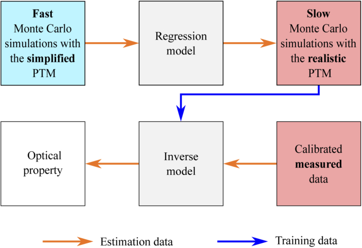
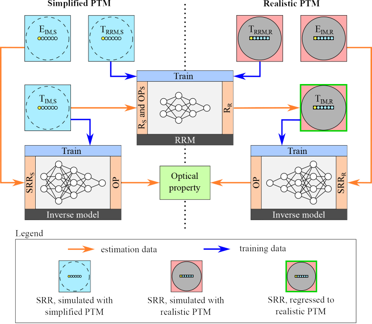
The basic idea of the methodology presented in this paper is summarized in Fig. 2. The SRR obtained by fast MC simulations utilizing a simplified PTM, which inaccurately describes the optical fiber probe tip and hence introduces errors into the simulated SRR, is rapidly transformed through the RRM to obtain accurate SRR. The accurate SRR can be also directly computed with MC simulations that utilize a realistic PTM, however such MC simulations are extremely slow. Detailed implementation of the RRM is discussed in Section 2.4 and the accuracy of the RRM is presented in Fig. 5. For additional numerical and experimental validation, the regressed reflectance was used to prepare inverse models for estimation of optical properties. Implementation details of the inverse models are presented in Section 2.5 and accuracy of the estimated optical properties is discussed in Section 3. A detailed workflow of the methodology that includes the RRM and inverse models is presented in Fig. 3.
Fig. 2.
Basic workflow of the proposed methodology. SRR that can be efficiently simulated with the simplified PTM but consequently subject to significant simulation errors is rapidly regressed to accurate SRR that could be directly obtained by much slower Monte Carlo simulations utilizing the realistic PTM. The regressed reflectance is used to substantially speed-up (up to 480 fold) the preparation of inverse models for estimation of optical properties from measured and calibrated SRR.
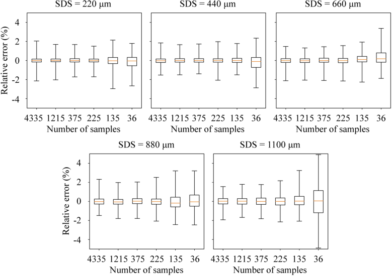
Fig. 5.
Distribution of the relative reflectance errors for the realistic PTM at 5 SDS obtained by the RRMs as a function of the training dataset size. The total number of SRR samples in the training datasets varies from 4335 (left) to 36 (right).
Fig. 3.
Illustration of the framework that includes training of the ANN-based RRMs that rapidly map SRR from the simplified PTM to the realistic PTM and training of the inverse models for estimation of optical properties from the SRR valid for the simplified or realistic PTMs. The and stand for reflectance at one source-detector separation, valid for the simplified and realistic PTMs, respectively. The and stand for the spatially resolved reflectance valid for the simplified and realistic PTM, respectively. The stands for optical property. (left) The SRRs simulated with the simplified PTM are passed through the inverse models for estimation of optical properties from the SRR valid for the simplified PTM. (right) The SRRs simulated with the realistic PTM are passed through the inverse models for estimation of optical properties from the SRR valid for the realistic PTM. Ideally, given that the RRM does not introduce additional errors into the regressed SRR, the estimation errors of the two inverse models should be similar and hence the inverse model of the simplified PTM serves as a performance baseline.
2.2. Light propagation model
In this study, the light propagation in sample was modeled by an experimentally validated OpenCLTM implementation of the MC method for a layered medium that follows the existing open source implementations [13,14]. All simulations of reflectance were prepared for an optical fiber probe with an outer diameter of 6.1 mm and six linearly placed optical fibers with a diameter of 200 µm and core-to-core spacing of 220 µm. Due to small source-detector separation (SDS), we took into account the so-called subdiffusive quantifiers of the scattering phase function (SPF), namely [15] and [16], as it has been shown, that they are important for accurate description of reflectance close to the source. Parameter is defined as a function of the first and second Legendre moments of SPF and is defined as a function of the first and third Legendre moments of SPF . The first Legendre moment is commonly termed as the anisotropy factor . Bodenschatz et al. demonstrated that higher-order Legendre moments carry information of large-angle scattering [17]. Two different approaches were used in the MC simulations to formulate the PTM that followed the work of Naglič et al. [18] (Fig. 1).
The first, simplified PTM, assumed a laterally uniform interface that took into account only the mismatch between the refractive indices of the sample (=1.33) and optical fibers (=1.452) [9]. Each MC simulation included at least photon packets that were launched uniformly with respect to the numerical aperture (NA=0.22) and diameter (200 µm) of the optical fiber core. To attain an acceptable and consistent signal-to-noise ratio of the SRR collected through the optical fibers, the MC simulations were terminated when the total weight of the photon packets, collected through the optical fiber with the largest SDS exceeded 1000. Due to the lateral uniformity of the PTM, the backscattered light was collected through a radially symmetric detection scheme (annual rings) centered at the position of the source optical fiber. The SRR collected through the 5 remaining fibers was derived from the output of the radially symmetric detection scheme.
The second, realistic PTM, accounted for the reflections from the polished stainless steel (0.5), the refractive index of the optical fibers ( = 1.452) [9] and the refractive index of the black epoxy resin ( = 1.6) (EpoTek 353ND Black, Epoxy Technology Inc., MA, USA), which were found to significantly affect the simulated reflectance [11,19]. Reflectivity of the stainless steel was measured by observing the attenuation of a reflected laser diode beam (670 nm) (Newport Optical Power Meter 1936-C and Thermopile Sensor 818P-001-12) and the reflectivity of the black epoxy resin was calculated by Fresnel’s equations. Once the photon packet hits the polished stainless steel or black epoxy surface of the probe tip, it reflects with a probability that equals reflectivity, otherwise it is considered completely absorbed Since the realistic PTM is not laterally uniform, the radial symmetry of the detection scheme breaks down and hence the reflectance was collected only through the individual optical fibers. To attain a signal-to-noise ratio of the simulated SRR similar to the simplified PTM, the minimum number of launched photon packets was increased by the ratio between the surface area of the most distant optical fiber and the corresponding annual ring of the radially symmetric detection scheme used for the simplified PTM. Consequently, at least photon packets were launched and the same MC termination criterion was used as for the simplified PTM.
2.3. Datasets
In this subsection we define the SRR datasets that were used to prepare and evaluate the RRM that maps the SRR valid for the simplified PTM to the SRR valid for the realistic PTM and the inverse models for estimation of optical properties. An overview of the datasets is provided in Table 1 and Fig. 3 shows the use of individual datasets within the proposed framework. Datasets denoted with letter T were utilized to train the ANN-based RMMs and inverse models, datasets denoted with letter V were utilized to control (validate) the training process and datasets denoted with letter E were used to test (independently evaluate) the trained ANNs. The range of optical properties was selected based on the values commonly reported for biological tissues [1,20–23]. However, the selected range can be customized to accommodate sample and application-specific requirements.
Table 1. Summary of datasets that includes the total number of SRR samples (), range of the optical properties (, , and ), source of the dataset (MC simulations or ANN-based reflectance regression model (RRM)) and probe tip model (PTM) complexity (simplified (S) or realistic (R)).
| Dataset name | (cm−1) | (cm−1) | Source | PTM | |||
|---|---|---|---|---|---|---|---|
| 108500 | 0.00-12.00 | 5.00-35.00 | 2.01-2.29 | 2.69-3.71 | MC | S | |
| 1680 | 0.19-11.82 | 5.30-32.85 | 2.06-2.27 | 2.84-3.68 | MC | S | |
| 512 | 0.00-12.00 | 5.00-35.00 | 2.09-2.20 | 2.83-3.52 | MC | S | |
|
| |||||||
| 4335 | 0.00-12.00 | 5.00-35.00 | 1.99-2.31 | 2.58-3.82 | MC | S | |
| 4335 | 0.00-12.00 | 5.00-35.00 | 1.99-2.31 | 2.58-3.82 | MC | R | |
| 1024 | 0.00-12.00 | 5.00-35.00 | 1.99-2.31 | 2.58-3.82 | MC | S | |
| 1024 | 0.00-12.00 | 5.00-35.00 | 1.99-2.31 | 2.58-3.82 | MC | R | |
|
| |||||||
| 108500 | 0.00-12.00 | 5.00-35.00 | 2.01-2.29 | 2.69-3.71 | RRM | R | |
| 1680 | 0.19-11.82 | 5.30-32.85 | 2.06-2.27 | 2.84-3.68 | RRM | R | |
| 512 | 0.00-12.00 | 5.00-35.00 | 2.09-2.20 | 2.83-3.52 | MC | R | |
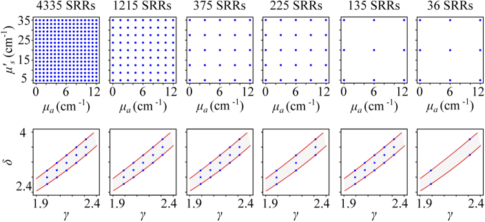
The points along the absorption coefficient () and reduced scattering coefficient () axes are equally spaced and form a regular grid in the plane. However, the points in the plane formed by the and subdiffuse SPF quantifiers are not located on a regular grid but are instead uniformly distributed in a way that includes the points that are laying on the boundary of the domain. We accomplish this by first uniformly distributing sample points along the axis within the selected range of values. At each sample point we compute intersections with the domain boundary of the GK [24] scattering phase function in the plane. The number of uniformly distributed sample points along the axis between the two intersections is selected in a way that keeps the distance between the sample points under a predefined value . Consequently, the total number of points in the plane is specified for each dataset. The distributions of sample points for all of the optical properties are presented in Fig. 4. All MC simulations of SRR were based on the Gegenbauer kernel (GK) [24] SPF. In the following, we provide a short description of the three groups of datasets summarized in Table 1.
Fig. 4.
Visualization of optical properties defined by the datasets summarized in Table 1. Red line shows the valid domain of and subdiffusive quantifiers for the GK scattering phase function.
-
1.Datasets that were used to prepare inverse models for estimation of optical properties from the SRR valid for the simplified PTM.
-
•The dataset was used to train the inverse models (35 equally spaced points along the axis, 50 equally spaced points along the axis and 62 points in the plane).
-
•The dataset was used to monitor the progress and stop the training of the inverse models (12 equally spaced points along the axis, 10 equally spaced points along the axis and 14 points in the plane).
-
•The dataset was used to independently evaluate the errors of the inverse models (8 equally spaced points along the axis, 8 equally spaced points along the axis and 8 points in the plane).
-
•
-
2.Datasets that were used to prepare RRMs that map SRR from the simplified to the realistic PTM.
-
•The and datasets were used to train the RRMs (17 equally spaced points along the axis, 17 equally spaced points along the axis and 15 points in the plane).
-
•The and datasets were used to independently evaluate the errors of the RRMs (8 equally spaced points along the axis, 8 equally spaced points along the axis and 16 points in the plane).
-
•
-
3.Datasets that were used to prepare inverse models for estimation of optical properties from the SRR valid for the realistic PTM.
-
•The dataset was regressed from the dataset and used to train the inverse models.
-
•The dataset was regressed from the dataset and used to monitor the progress and stop the training of the inverse models.
-
•The dataset was used to independently evaluate the errors of the inverse models.
-
•
2.4. Reflectance regression model (RRM)
The RRMs that map SRR from the simplified PTM to the realistic PTM were based on deep ANNs. One ANN model was trained for each SDS. The five inputs of the ANN-based RRMs were formed by the reflectance value at the selected SDS and the corresponding absorption coefficient , reduce scattering coefficient and SPF quantifiers and . The output of each ANN-based RRM was defined as the relative difference between the reflectance values at the selected SDS that were simulated with the simplified and the realistic PTM. The regression ANNs were trained using the dataset as the input and the relative difference between and as the output. A small three-layer deep ANN topology was used with 8, 4 and 1 nodes in the individual layers. A softplus activation function was applied to the first two layers and a hard-sigmoid activation function to the output layer. The training datasets and were gradually reduced in size as summarized in Table 2 and shown in Fig. 4 to obtain an estimate for the smallest dataset that is required to train sufficiently accurate RRMs.
Table 2. Summary of the decimated and datasets used to train the ANN-based RRMs that map SRR from the simplified PTM to the realistic PTM.
| Total number of SRR samples |
||||||
|---|---|---|---|---|---|---|
| Parameter | 4335 | 1215 | 375 | 225 | 135 | 36 |
| 17 | 9 | 5 | 5 | 3 | 3 | |
| 17 | 9 | 5 | 5 | 3 | 3 | |
| 5 | 5 | 5 | 3 | 5 | 2 | |
| 3 | 3 | 3 | 3 | 3 | 2 | |
The training of the ANNs was based on the Adam optimizer [25] using mean squared error cost function and fixed learning rate of . Due to the stochastic nature of the training process, 10 RRMs were trained for each SDS and dataset size. Subsequently, the model with the lowest regression error on the dataset was selected.
2.5. Inverse models
Dedicated ANN-based inverse models for estimation of optical properties from SRR were prepared for the simplified PTM and for the realistic PTM. The inverse models were prepared following our methodology presented in [26]. The inverse models for the simplified and realistic PTM were trained using the and datasets, respectively. The inputs of each inverse model were formed by the 5 SRR values collected through the optical fibers and one output represented the estimated optical property. A five-layer deep ANN topology was used with 30, 20, 10, 5 and 1 nodes in the individual layers. A linear activation function was used in the first layer, a hyperbolic tangent activation function was used in the hidden layers and a hard-sigmoid activation function was used in the output layer. The training of the ANNs was based on the Adam optimizer [25] using mean squared error cost function and adaptive learning rate that exponentially decayed with the number of training epochs . The training process was limited to 10000 epochs and was stopped early if the value of the cost function on a small validation dataset, for the simplified PTM and for the realistic PTM, did not sufficiently improve for 500 consecutive training epochs. Due to the stochastic nature of the training process, 5 inverse models were trained for each optical property and PTM. Subsequently, the inverse model with the lowest estimation error was selected. For notation simplicity, the inverse models prepared for the simplified PTM will be referred to as and the inverse models prepared for the realistic PTM will be referred to as , where n stands for the number of SRRs used to train the underlying RRM that produced the correspondent dataset (e.g. )
2.6. Turbid phantoms
We prepared five liquid turbid phantoms comprising a mixture of absorbers and scatterers following the procedure described in [18]. A green molecular dye found in fountain pen inks (Live Line Green) was used as the absorber. A 10 mm cuvette (Hellma Optik GmbH, Jena, Germany) and a cuvette holder (CUV-UV/VIS, Avantes, Apeldoorn, The Netherlands) were used to measure the absorption coefficient of diluted molecular dye by applying Beer-Lambert law to the attenuation of a collimated light beam, transmitted through the cuvette. Aqueous suspensions of µm and µm polysterene particles (microParticles GmbH, Berlin, Germany) were used as scatterers. The scattering coefficient and SPF quantifiers and of the liquid suspensions were computed using the Mie theory and the wavelength dependence of the polystyrene refractive index was taken from [27]. The MC simulations of turbid phantoms required numerical sampling of the scattering angles, which was implemented as detailed in [28]. The optical properties of the five turbid phantoms are summarized in Table 3.
Table 3. The range of optical properties (, , and ) spanned by the five liquid turbid phantoms (TP) that were prepared to experimentally validate the inverse models and the average diameter and standard deviation of polystyrene particles in the individual turbid phantoms.
| TP | (cm−1) | (cm−1) | (µm) | (µm) | ||
|---|---|---|---|---|---|---|
| 0.00 | 28.08-34.05 | 1.53-1.93 | 2.23-2.95 | 2.56 | 0.04 | |
| 0.00 | 18.71-22.69 | 1.53-1.93 | 2.23-2.95 | 2.56 | 0.04 | |
| 0.00 | 9.38-11.37 | 1.53-1.93 | 2.23-2.95 | 2.56 | 0.04 | |
|
| ||||||
| 0.00-4.72 | 17.24-25.43 | 2.03-2.27 | 3.10-3.55 | 0.525 | 0.01 | |
| 0.00-4.72 | 8.63-12.73 | 2.03-2.27 | 3.10-3.55 | 0.525 | 0.01 | |
2.7. Experimental setup
Experimental validation was based on liquid turbid phantoms with known optical properties. The turbid phantoms were poured into a cylindrical beaker with a diameter of 19.5 mm and a height of 30 mm, coated with a black matte paint to reduce reflections from walls and stray light pollution. A custom-made linear array optical fiber probe (FiberTech Optica Inc., Ontario, Canada) with a 6.1 mm stainless steel housing and six 200 µm optical fibers (220, 440, 660, 880, and 1100 µm SDS) was dipped about 5 mm deep into the turbid phantoms. The turbid phantoms were illuminated by the first optical fiber that was coupled to a broadband halogen light source (AvaLight-Hal LS, Avantes, Apeldoorn, The Netherlands). The backscattered light collected through the remaining five optical fibers was dispersed onto a camera (acA1920-150um, Basler, Ahrensburg, Germany) by a fiber-coupled imaging spectrograph (ImSpector V10E, 400-1000 nm, Specim, Spectral Imaging Ltd., Oulu, Finland). The measured spectra were corrected for the dark response of the sensor array and normalized by the dark corrected reflectance of a standard diffuse tile (WS-2, Avantes, Apeldoorn, The Netherlands). A more detailed description of the measurement setup can be found in [29].
3. Results and discussion
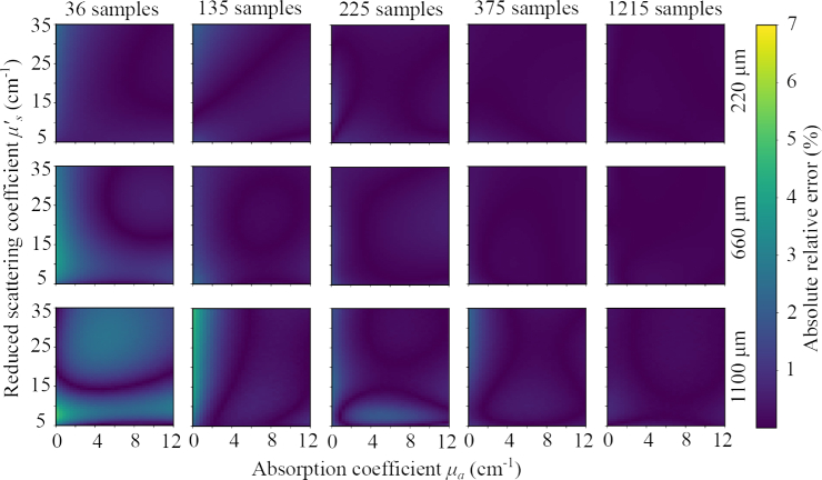
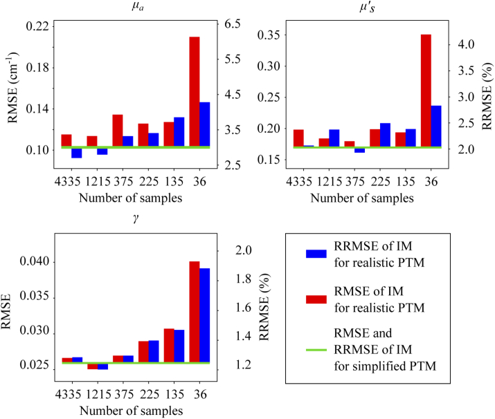
The training process of RRMs was repeated 10 times for each dataset size summarized in Table 2 and visualized in Fig. 4. The best RRM was selected based on the mean absolute relative error between the regressed and simulated SRR datasets. The relative errors of the RRM as a function of the number of SRR samples in the training set is summarized in Fig. 5. The SRR regression errors begin to significantly increase if the training dataset is reduced to less than 225 SRR samples. The error maps in Fig. 6 provide visualization of the reflectance errors as a function of the optical properties. The relative errors shown in the maps were computed with respect to the reflectance values obtained by RRMs that were trained by the full size of the training dataset with 4335 SRR samples. The calculated errors are unbiased and start to significantly increase only for the two smallest training datasets with merely 135 and 36 SRR samples. To further validate the performance of the RRMs that map SRR from the simplified to the realistic PTM, we trained seven sets of inverse models for estimation of optical properties, namely , , , , , , . The errors of optical properties , and estimated by the inverse models were independently evaluated using the dataset for and dataset for through (Fig. 7). The evaluation results confirm, that a small training set of merely 225 SRR samples is enough to prepare sufficiently accurate RRMs and from there inverse models () for estimation of optical properties.
Fig. 6.
Absolute relative error maps of reflectance that was regressed from SRR valid for the simplified PTM to SRR valid for the realistic PTM as a function of the number of SRR samples that were used to train the ANN-based RRMs. The relative errors are provided for three SDS, namely (first row) 220 µm, (second row) 660 µm and (third row) 1100 µm.
Fig. 7.
Root mean square errors (RMSE) and relative root mean square errors (RRMSE) of the absorption coefficient , reduced scattering coefficient and SPF quantifier , estimated by inverse models for the realistic PTM as a function of the size (4335, 1215, 375, 225, 135 and 36 SRR samples) of the dataset that was used to train the underlying RRM. Green line shows the performance of the inverse model for the simplified PTM that does not depend on the properties of the RRM and thus serves as a baseline.
To highlight the computational efficiency of the proposed regression framework, we measured the MC simulation times required to prepare SRRs of comparable quality at 16 points representing the corners of the dataset using the simplified and realistic PTMs. The MC simulations for the simplified PTM were terminated when the total weight of the photon packets collected through the annual ring representing the optical fiber with the largest SDS exceeded 1000. Likewise, the MC simulations for the realistic PTM were terminated when the total weight of the photon packets collected through the optical fiber with the largest SDS exceeded 40000. The two termination criteria produced reflectance of comparable quality on the most distant optical fiber. The MC simulations on NvidiaTM Geforce GTX 1070 GPU took 242 s for the simplified PTM and 9533 s for the realistic PTM. The ratio between the two computational times tightly follows the ratio between the surface areas of the optical fiber and of the corresponding annual ring. The time required by the RRM to map the SRR from the simplified to the realistic PTM was found negligible. Since an accurate RRM that maps SRR from the simplified PTM to the realistic PTM can be derived from a small training dataset of merely 225 SRR samples, the total time required to prepare is further reduced by a factor of (given that a training dataset for a simplified PTM is readily available).
From the timing data (Nvidia GTX 1070) we can estimate that the preparation of the datasets required to deploy the RRM in our study takes 19 days for , 1.5 days for and 1 hour for (assuming that the datasets used to train the RRM contain 225 SRR samples). In contrast, without using the proposed RRM, the simulations of dataset, required to prepare the inverse models for realistic PTM, would take about 748 days.
To demonstrate the additional noise reduction attained with the proposed framework, we compared the spread of 100 reflectances simulated with the realistic PTM to the spread of 100 reflectances simulated with the simplified PTM and regressed to reflectances valid for the realistic PTM. The simulations were performed with photon packets for a selection of optical properties that exhibits the highest simulation noise: = 12 cm−1, = 5 cm−1, and . The results presented in Fig. 8 show that the spread of reflectances valid for the realistic PTM is much smaller for the regressed reflectances that benefit from the radially symmetric detection scheme used in the MC simulations for simplified PTM. Note that the average values of the simulated and regressed reflectances match almost perfectly.
Fig. 8.
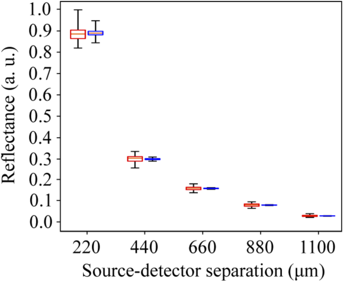
Spread of 100 reflectance points simulated with the realistic PTM (red) and spread of 100 reflectance points simulated with the simplified PTM and regressed to the realistic PTM (blue). The reflectance points were simulated for optical properties ( = 12 cm−1, = 5 cm−1, and ) that were found to produce the noisiest reflectance.
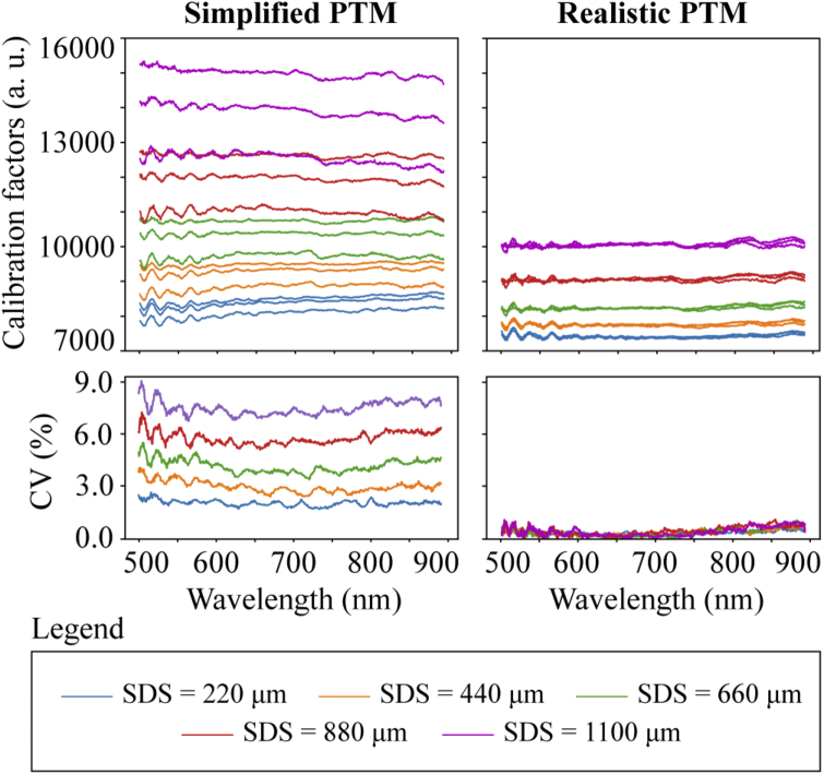
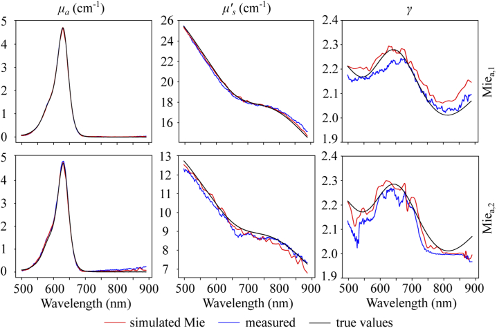
Finally, we validated the proposed framework experimentally. For this purpose, two sets of measurements were collected from nonabsorbing and absorbing liquid turbid phantoms with well-defined optical properties summarized in Table 3. The nonabsorbing liquid phantoms were prepared using 2.56 µm polystyrene spheres and the absorbing phantoms were prepared using 0.525 µm polystyrene spheres and a green molecular absorber. The calibration factors that map the MC simulated SRR to the measured SRR were computed by dividing the MC simulated SRRs of nonabsorbing liquid phantoms and the corresponding measured SRRs. Ideally, the values of calibration factors at a given SDS should be the same for all the turbid phantoms. The values of calculated calibration factors for the 5 SDSs are shown in Fig. 9. The top row shows the calibration factors calculated from reflectance of optical phantoms simulated with the simplified (left) and realistic PTM (right) at each SDS. The bottom row shows the corresponding coefficients of variation (CV) for the calibration factors. One can clearly see that the calibration factors computed from the reflectance simulated with the simplified PTM do not match within a particular SDS and are biased in comparison to the calibration factors computed from the reflectance simulated with the realistic PTM. From there it follows that the CV of the calibration factors computed from the reflectance simulated with the simplified PTM is nearly 10%, while the CV of the calibration factors computed from the reflectance simulated with the realistic PTM is merely 1%. Further analysis and discussion on the sources of the observed mismatch and bias of the calibration factors computed from the reflectance simulated with the simplified PTM can be found in [11]. Consequently, the calibration factors at each SDS were smoothed by fitting a second-order polynomial to the calibration factors as a function of wavelength. The calibrated measured reflectances of the absorbing liquid phantoms and were passed through the inverse models . The SRR of the absorbing turbid phantoms for the realistic PTM were also simulated using the expected values of optical properties and the Mie or GK SPFs. The parameters of GK SPF and were calculated by matching the values of and of the Mie SPF that holds for the liquid phantoms. Note, that some pairs of and values cannot be attained by the GK SPF and were thus omitted from the SRR simulations. The optical properties estimated from the simulated SRR served as a baseline for the optical properties estimated from the measured SRR. The estimated values of optical properties are shown in Fig. 10 and the estimation errors are summarized in Table 4. The obtained RMSE and RRMSE errors of the estimated optical properties are similar for the simulated and the measured SRR, which indicates that the inverse models are unbiased. A slightly higher error of the estimated optical properties can be observed for the turbid phantom (measured and simulated SRR), in particular at longer wavelengths, where the values of drop bellow 9 cm−1. The slightly increased errors could be explained by the influence of the SPF on the reflectance that is stronger at low values, where the GK SPF that was used to simulate the training datasets of the inverse models cannot sufficiently account for the details of the Mie SPF that holds for the turbid phantoms.
Fig. 9.
(top) Reflectance calibration factors for five SDS calculated from reflectance simulated with the simplified and realistic PTM for three non-absorbing liquid turbid phantoms , and . (bottom) Coefficient of variation (CV) for the calibration factors at each SDS for the simplified and realistic PTM.
Fig. 10.
Optical properties of the and turbid phantoms, predicted by . Red lines - optical properties estimated from SRR simulated with the Mie SPF using the realistic PTM, blue lines - optical properties estimated from the measured SRR, black lines - true/expected values of the optical properties.
Table 4. Root mean square (RMSE) and relative root mean square (RRMSE) errors of optical properties estimated for the (top rows) and (bottom rows) absorbing turbid phantom from the SRR simulated with the GK and Mie SPFs using the realistic PTM, and from measured SRR.
| Optical property | Simulated GK | Simulated Mie | Measured |
|---|---|---|---|
| RMSE(RRMSE) | RMSE(RRMSE) | RMSE(RRMSE) | |
| (cm−1) | 0.023 | 0.030 | 0.022 |
| 0.032 | 0.066 | 0.094 | |
|
| |||
| (cm−1) | 0.10 (0.58%) | 0.13 (0.71%) | 0.30 (1.69%) |
| 0.14 (1.65%) | 0.22 (2.60%) | 0.25 (2.51%) | |
|
| |||
| 0.015 (0.75%) | 0.033 (1.53%) | 0.027 (1.26%) | |
| 0.023 (1.10%) | 0.029 (1.38%) | 0.050 (2.32%) | |
Accurate MC simulation of reflectance for optical fiber probes are challenging and require careful consideration of all the details in the simulation model, in particular if used for estimation of optical properties by inverse models [11]. At small SDS that are frequently used with optical fiber probes, the inverse models need to take into account additional scattering phase function quantifiers such as and , which are related to second and third Legendre moments of the SPF, respectively. The additional parameters significantly increase the number of MC simulations required to prepare inverse models for estimation of optical properties. Furthermore, if a realistic description of the PTM is also used in the MC simulations, the symmetry of the detection scheme breaks down and the number of photon packets required for good quality SRRs further increases by about two orders of magnitude. Consequently, the total simulation time required to prepare datasets becomes excessively long and impractical even when using the latest generation GPUs. To overcome these limitations, many existing studies have used a simplified PTM [9,10,30–32], eventhough it has been shown [1,11,12] that such simplifications lead to large simulation errors of SRR. The proposed framework overcomes these limitations, and allows simulation of SRR using a realistic PTM at the speed and quality that matches MC simulations with a simplified PTM. The additional computational steps are based on efficient and accurate deep ANN-based RRMs, with negligible computational overhead. The proposed framework can be particularly beneficial for applications that utilize a linear layout of optical fibers in the probe, since the effect of the PTM on the reflectance [11] has been shown to increase with the SDS.
We believe that the presented framework can be applied to different measurement settings and in general take the efficiency and quality of MC simulations to a new level.
4. Conclusions
In this paper we present an efficient framework for MC simulation of SRR, that accounts for all the details of the optical fiber probe tip. For this purpose, we used deep neural networks that map the SRR, simulated with the simplified PTM to SRR, simulated with the realistic PTM. The results of the RRM were extensively validated through the use of inverse models for estimation of optical properties from simulated SRR and measured SRR of turbid phantoms. The results show that 225 SRR samples are sufficient to derive an accurate deep ANN-based RRM, which is about 480-fold less than the number of SRRs (108500) required to train a typical inverse model for estimation of optical properties. The remaining SRR samples can be efficiently simulated with the simplified PTM and rapidly regressed to SRR valid for the realistic PTM. Using the proposed methodology, it is possible to prepare high-quality inverse models for realistic PTM in approximately the same time as for simplified PTM.
Funding
Javna Agencija za Raziskovalno Dejavnost RS10.13039/501100004329 (J2-7211, J2-8173, P2-0232).
Disclosures
The authors declare no conflicts of interest.
References
- 1.Bevilacqua F., Piguet D., Marquet P., Gross J. D., Tromberg B. J., Depeursinge C., “In vivo local determination of tissue optical properties: applications to human brain,” Appl. Opt. 38(22), 4939–4950 (1999). 10.1364/AO.38.004939 [DOI] [PubMed] [Google Scholar]
- 2.Ivancic M., Naglic P., Pernus F., Likar B., Burmen M., “Extraction of optical properties from hyperspectral images by Monte Carlo light propagation model,” in Optical Interactions with Tissue and Cells Xxvii, vol. 9706 Jansen E. D., ed. (Spie-Int Soc Optical Engineering, Bellingham, 2016), p. 97061A [Google Scholar]
- 3.Wang L. V., Wu H.-i., Biomedical optics: principles and imaging (John Wiley & Sons, 2012). [Google Scholar]
- 4.Vitkin E., Turzhitsky V., Qiu L., Guo L., Itzkan I., Hanlon E. B., Perelman L. T., “Photon diffusion near the point-of-entry in anisotropically scattering turbid media,” Nat. Commun. 2(1), 587 (2011). 10.1038/ncomms1599 [DOI] [PMC free article] [PubMed] [Google Scholar]
- 5.Liemert A., Kienle A., “Exact and efficient solution of the radiative transport equation for the semi-infinite medium,” Sci. Rep. 3(1), 2018 (2013). 10.1038/srep02018 [DOI] [PMC free article] [PubMed] [Google Scholar]
- 6.Kienle A., Patterson M. S., “Improved solutions of the steady-state and the time-resolved diffusion equations for reflectance from a semi-infinite turbid medium,” J. Opt. Soc. Am. A 14(1), 246–254 (1997). 10.1364/JOSAA.14.000246 [DOI] [PubMed] [Google Scholar]
- 7.Zhu C., Liu Q., Ramanujam N., “Effect of fiber optic probe geometry on depth-resolved fluorescence measurements from epithelial tissues: a Monte Carlo simulation,” J. Biomed. Opt. 8(2), 237 (2003). 10.1117/1.1559058 [DOI] [PubMed] [Google Scholar]
- 8.Palmer G. M., Ramanujam N., “Monte Carlo-based inverse model for calculating tissue optical properties. Part I: Theory and validation on synthetic phantoms,” Appl. Opt. 45(5), 1062–1071 (2006). 10.1364/AO.45.001062 [DOI] [PubMed] [Google Scholar]
- 9.Hennessy R., Lim S. L., Markey M. K., Tunnell J. W., “Monte Carlo lookup table-based inverse model for extracting optical properties from tissue-simulating phantoms using diffuse reflectance spectroscopy,” J. Biomed. Opt. 18(3), 037003 (2013). 10.1117/1.JBO.18.3.037003 [DOI] [PMC free article] [PubMed] [Google Scholar]
- 10.Fredriksson I., Larsson M., Stromberg T., “Inverse Monte Carlo method in a multilayered tissue model for diffuse reflectance spectroscopy,” J. Biomed. Opt. 17(4), 047004 (2012). 10.1117/1.JBO.17.4.047004 [DOI] [PubMed] [Google Scholar]
- 11.Naglic P., Pernus F., Likar B., Buermen M., “Limitations of the commonly used simplified laterally uniform optical fiber probe-tissue interface in Monte Carlo simulations of diffuse reflectance,” Biomed. Opt. Express 6(10), 3973–3988 (2015). 10.1364/BOE.6.003973 [DOI] [PMC free article] [PubMed] [Google Scholar]
- 12.Cappon D. J., Farrell T. J., Fang Q., Hayward J. E., “Fiber-optic probe design and optical property recovery algorithm for optical biopsy of brain tissue,” J. Biomed. Opt. 18(10), 107004 (2013). 10.1117/1.JBO.18.10.107004 [DOI] [PubMed] [Google Scholar]
- 13.Wang L., Jacques S., Zheng L., “Mcml - Monte-Carlo Modeling of Light Transport in Multilayered Tissues,” Comput. Methods Programs Biomed. 47(2), 131–146 (1995). 10.1016/0169-2607(95)01640-F [DOI] [PubMed] [Google Scholar]
- 14.Alerstam E., Svensson T., Andersson-Engels S., “Parallel computing with graphics processing units for high-speed Monte Carlo simulation of photon migration,” J. Biomed. Opt. 13(6), 060504 (2008). 10.1117/1.3041496 [DOI] [PubMed] [Google Scholar]
- 15.Bevilacqua F., Depeursinge C., “Monte Carlo study of diffuse reflectance at source-detector separations close to one transport mean free path,” J. Opt. Soc. Am. A 16(12), 2935–2945 (1999). 10.1364/JOSAA.16.002935 [DOI] [Google Scholar]
- 16.Tian H. J., Liu Y., Wang L. J., “Influence of the third-order parameter on diffuse reflectance at small source-detector separations,” Opt. Lett. 31(7), 933–935 (2006). 10.1364/OL.31.000933 [DOI] [PubMed] [Google Scholar]
- 17.Bodenschatz N., Krauter P., Liemert A., Kienle A., “Quantifying phase function influence in subdiffusively backscattered light,” J. Biomed. Opt. 21(3), 035002 (2016). 10.1117/1.JBO.21.3.035002 [DOI] [PubMed] [Google Scholar]
- 18.Naglic P., Pernus F., Likar B., Burmen M., “Estimation of optical properties by spatially resolved reflectance spectroscopy in the subdiffusive regime,” J. Biomed. Opt. 21(9), 095003 (2016). 10.1117/1.JBO.21.9.095003 [DOI] [PubMed] [Google Scholar]
- 19.Naglic P., Pernus F., Likar B., Buermen M., “Adopting higher-order similarity relations for improved estimation of optical properties from subdiffusive reflectance,” Opt. Lett. 42(7), 1357–1360 (2017). 10.1364/OL.42.001357 [DOI] [PubMed] [Google Scholar]
- 20.Sandell J. L., Zhu T. C., “A review of in-vivo optical properties of human tissues and its impact on PDT,” J. Biophotonics 4(11-12), 773–787 (2011). 10.1002/jbio.201100062 [DOI] [PMC free article] [PubMed] [Google Scholar]
- 21.Bevilacqua F., Berger A. J., Cerussi A. E., Jakubowski D., Tromberg B. J., “Broadband absorption spectroscopy in turbid media by combined frequency-domain and steady-state methods,” Appl. Opt. 39(34), 6498 (2000). 10.1364/AO.39.006498 [DOI] [PubMed] [Google Scholar]
- 22.Thueler P., Charvet I., Bevilacqua F., St. Ghislain M., Ory G., Marquet P., Meda P., Vermeulen B., Depeursinge C., “In vivo endoscopic tissue diagnostics based on spectroscopic absorption, scattering, and phase function properties,” J. Biomed. Opt. 8(3), 495 (2003). 10.1117/1.1578494 [DOI] [PubMed] [Google Scholar]
- 23.Bashkatov A. N., Genina E. A., Tuchin V. V., “Optical properties of skin, subcutaneous, and muscle tissues: a review,” J. Innovative Opt. Health Sci. 04(01), 9–38 (2011). 10.1142/S1793545811001319 [DOI] [Google Scholar]
- 24.Reynolds L., Mccormick N., “Approximate 2-Parameter Phase Function for Light-Scattering,” J. Opt. Soc. Am. 70(10), 1206–1212 (1980). 10.1364/JOSA.70.001206 [DOI] [Google Scholar]
- 25.Chollet F., Deep learning with python (Manning Publications Co., 2017). [Google Scholar]
- 26.Ivancic M., Naglic P., Pernus F., Likar B., Burmen M., “Efficient estimation of subdiffusive optical parameters in real time from spatially resolved reflectance by artificial neural networks,” Opt. Lett. 43(12), 2901–2904 (2018). 10.1364/OL.43.002901 [DOI] [PubMed] [Google Scholar]
- 27.Nikolov I. D., Ivanov C. D., “Optical plastic refractive measurements in the visible and the near-infrared regions,” Appl. Opt. 39(13), 2067–2070 (2000). 10.1364/AO.39.002067 [DOI] [PubMed] [Google Scholar]
- 28.Naglia P., Pernua F., Likar B., Burmen M., “Lookup table-based sampling of the phase function for Monte Carlo simulations of light propagation in turbid media,” Biomed. Opt. Express 8(3), 1895–1910 (2017). 10.1364/BOE.8.001895 [DOI] [PMC free article] [PubMed] [Google Scholar]
- 29.Naglic P., Ivancic M., Pernus F., Likar B., Burmen M., “Portable measurement system for real-time acquisition and analysis of in-vivo spatially resolved reflectance in the subdiffusive regime,” Design and Quality for Biomedical Technologies Xi, vol. 10486 Raghavachari R., Liang R., eds. (Spie-Int Soc Optical Engineering, Bellingham, 2018), p. UNSP 1048618. [Google Scholar]
- 30.Einstein G., Aruna P., Ganesan S., “Monte Carlo based model for diffuse reflectance from turbid media for the diagnosis of epithelial dysplasia,” Optik 181, 828–835 (2019). 10.1016/j.ijleo.2018.12.158 [DOI] [Google Scholar]
- 31.Sharma M., Hennessy R., Markey M. K., Tunnell J. W., “Verification of a two-layer inverse Monte Carlo absorption model using multiple source-detector separation diffuse reflectance spectroscopy,” Biomed. Opt. Express 5(1), 40–53 (2014). 10.1364/BOE.5.000040 [DOI] [PMC free article] [PubMed] [Google Scholar]
- 32.Zhong X., Wen X., Zhu D., “Lookup-table-based inverse model for human skin reflectance spectroscopy: two-layered Monte Carlo simulations and experiments,” Opt. Express 22(2), 1852–1864 (2014). 10.1364/OE.22.001852 [DOI] [PubMed] [Google Scholar]


