Abstract
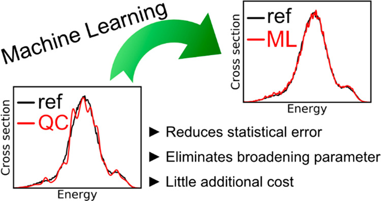
We present a machine learning (ML) method to accelerate the nuclear ensemble approach (NEA) for computing absorption cross sections. ML-NEA is used to calculate cross sections on vast ensembles of nuclear geometries to reduce the error due to insufficient statistical sampling. The electronic properties—excitation energies and oscillator strengths—are calculated with a reference electronic structure method only for a relatively few points in the ensemble. The KREG model (kernel-ridge-regression-based ML combined with the RE descriptor) as implemented in MLatom is used to predict these properties for the remaining tens of thousands of points in the ensemble without incurring much of additional computational cost. We demonstrate for two examples, benzene and a 9-dicyanomethylene derivative of acridine, that ML-NEA can produce statistically converged cross sections even for very challenging cases and even with as few as several hundreds of training points.
Introduction
Absorption spectroscopy is an essential tool for chemists because it allows the characterization of electronic properties of materials and helps determine the chemical structure of synthesized compounds. Quantum chemistry (QC) provides an arsenal of valuable methods to simulate electronically excited states to understand the nature of observed spectral features better, allowing, for instance, distinguishing between plausible structures of synthesized species. Such QC methods also allow predicting properties of yet-to-be-prepared compounds, e.g., in high-throughput screening, circumventing the need for resource-intensive and time-consuming experimental preparation and screening of compounds.1
QC methods for absorption spectrum simulation can be classified in terms of the type of approach to spectrum calculations and the electronic-structure method employed. Both determine the computational cost, precision, and accuracy of the spectrum simulation. The researcher must opt for a computational setup that allows an acceptable trade-off between accuracy and computational cost. From the spectrum simulation methodology, the cost/accuracy trade-off spans from simple stick spectra2 based on vertical excitations to high-level spectroscopic simulations with time-dependent3,4 and time-independent5 methods with vibrational resolution and vibronic couplings. On the other hand, from the electronic-structure standpoint, this trade-off goes all the way from energy differences between frontier Kohn–Sham orbitals with the relatively inexpensive density functional theory (DFT), which may be useful for instance for high-throughput screening,1 to high-level multireference quantum chemistry of small molecules.6 Between these extremes, a reasonable compromise can be reached calculating the main spectral inhomogeneous features with a method like the nuclear ensemble approach (NEA),7 using electronic information computed at relatively low-cost single-reference methods like the linear-response time-dependent DFT (TDDFT).8
Using NEA for simulating the absorption spectra of molecules requires the calculation of energies and oscillator strengths for many (often dozens) electronic states in the spectroscopically relevant region for hundreds or even thousands of geometries in an ensemble representing the nuclear distribution in the ground state. It allows obtaining a description of the absorption cross section, including absolute band envelopes (without vibrational resolution) of bright and dark bands. NEA is also often used to sample initial conditions to initiate mixed quantum-classical dynamics.9,10
The computational cost of the large number of electronic structure calculations required in NEA may become unaffordable for large molecules, even when based on TDDFT employing double-ζ basis sets. Thus, NEA is usually only used for small to medium molecules, being out of range for most of the systems of applied interest. Moreover, when dealing with rare events,11 the sampling space may become unaffordable even for medium-sized molecules.12
The reduction of the computational cost is paramount for allowing routine calculations of the absorption cross section with NEA. A first strategy for this cost reduction is to adopt stronger approximations of QC methods. It may, however, lead to an inadequate description of the electronic transitions. An alternative strategy is offered by machine learning (ML), which can substitute substantial parts of QC calculations and deliver predictions without much loss of accuracy.13−15 Encouragingly, ML has been already applied in excited-state simulations.16−36 In particular, ML-accelerated NEA has been proposed by Ye and co-workers, who employed neural networks to predict excitation energies, ground-state dipole moments, and transition dipole moments to simulate absorption spectra of a small molecule at different temperatures based on ensembles built via molecular dynamics (MD).20 Alternatively, ensembles can be built via normal mode sampling as is done for generating initial training sets of machine learning potential energy models, which are later refined by active learning.25−27,37
In this study, we follow exploring this second strategy, developing a different ML technique for substantially accelerating the calculation of NEA absorption cross sections. In our method, the KREG model (kernel-ridge-regression (KRR) ML with RE descriptor; see Methods for details)15,38,39 is used for calculating excited-state energies and oscillator strengths for tens of thousands of points in the nuclear ensemble, while being trained only on a tiny fraction of points of this ensemble, calculated with a QC method. The ensembles are built on geometries sampled from a Wigner distribution, which results in more accurate spectra than those from MD ensembles.40 These ensembles are, however, more challenging to be modeled, as they have a much wider variability of geometries. Yet, we show that the precision of the resulting ML-NEA cross sections is significantly improved compared to that of QC cross sections calculated with far fewer points in the ensemble.
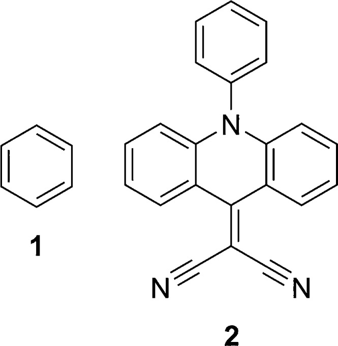
In the following, we describe the methodology behind the ML-NEA, and then, we demonstrate the application of this approach on a couple of examples, benzene and a large 9-dicyanomethylene derivative of acridine ((10-phenylacridin-9(10H)-ylidene)malononitrile, Chart 1). Benzene was chosen because it is a small, well-studied molecule that can be pressed to the limit to test the ML and QC methods. Moreover, the absorption cross sections of its three first absorption bands span 4 orders of magnitude, which makes benzene a particularly challenging system. In turn, compound 2 illustrates the potential of the method for a molecule already too large to apply pure QC-NEA routinely.
Chart 1. Structures of Compounds Used in This Study: 1, Benzene with 12 Atoms; 2, 9-Dicyanomethylene Derivative of Acridine with 38 Atoms.
Methods
In the NEA, the absorption cross section σ(E) at excitation energy E is calculated as7
 |
1 |
where, as usual, e and m are the electron charge and mass, c is the speed of the light, ε0 is the vacuum permittivity, and ℏ is the reduced Planck constant. The sums run over Nfs excited states and Np nuclear geometries xi. For each of such geometries in the ensemble, transition energies ΔE0n(xi) and oscillator strengths f0n(xi) between the ground (0) and the excited (n) states are computed. Each transition in the ensemble is convoluted with a normalized line shape function centered at ΔE0n(xi) and with width δ. In this work, the line shape function is a normalized Gaussian function given by
| 2 |
Although δ is an arbitrary parameter, it must be much narrower than the bandwidth, so as not to interfere in its description. As the average value of band widths is around 0.3 eV,2 it is a good practice to adopt δ ≤ 0.05 eV.
An NEA spectrum simulation consists of three steps. The first one is to create an ensemble of Np nuclear geometries (xi) around the minimum of the initial state (for an absorption spectrum, the ground state). Such an ensemble can be created via different procedures, distributions (like Wigner), MD simulations, and even hybrid combinations.41 The ML-NEA method we propose here can be used with any kind of ensemble. In this work, we have used Wigner sampling because it is our routine methodology. For single isolated molecules, we consider it superior to MD because it accounts for the zero-point energy of the initial state, while MD does not (see ref 40). Computationally, sampling geometries with a Wigner distribution is inexpensive, and we can do it for as many points as we want. The second step to simulate an NEA spectrum is to compute excitation energies and transition probabilities for each geometry in the ensemble (in the case of an absorption spectrum, ΔE0n(xi) and f0n(xi) as shown in eq 1). Here, the computational costs kicks in. It may be unaffordable to carry out tens of thousands of such electronic structure calculations with a quantum chemical method. The goal of our work is exactly to show how to replace most of these QC calculations by ML ones. The third and final step in the NEA simulation is to perform the sums in eq 1, which is, once more, computationally inexpensive.
More technically, the molecular geometries xi of the nuclear ensemble are stochastically obtained in this study from a Wigner distribution for the quantum harmonic approximation of the vibrational normal modes.42 For a molecule with Nat atoms, Np random geometries qi are generated by sampling normal-mode coordinate qik and momentum pik using the distribution
| 3 |
where
 |
4 |
In eq 3, the product is evaluated over the 3Nat – 6 normal modes k, each one with reduced mass μk and angular frequency ωk. The momentum values are not used for the spectrum simulations, but they are useful when the ensemble is used as initial conditions for dynamics. After the sampling, each qi is converted into Cartesian coordinates xi, which are used for computing ΔE0n(xi) and f0n(xi) appearing in eq 1.
As expressed in eq 1, to calculate the cross section, only excitation energies ΔE and oscillator strengths f are necessary (here and in the following, we dropped the indices and the dependence on xi for clarity). They are usually obtained using electronic-structure QC method such as TDDFT. To obtain the absorption cross section with a low error due to the statistical sampling, such electronic-structure calculations are necessary for many electronic excitations and large number (hundreds or thousands) of geometries. Thus, precise and accurate NEA cross section calculation requires using significant computational resources, as discussed in the Introduction.
Here, we suggest replacing
most of QC calculations by ML ones.
We train individual ML models for each excitation energy ΔE and oscillator strength f on Ntr points out of a vast ensemble of 50000 geometries
(50k-ensemble in the following). Then, we use these ML models to predict
these quantities for the remaining geometries in the 50k-ensemble
essentially for free in terms of computational time. Each ML model
is a kernel ridge regression (KRR) model using the Gaussian kernel
function  and the vector of normalized inversed internuclear
distances (RE) as the molecular descriptor x (input vector).15,38,39 We call this combination the
KREG model. It allows for obtaining potential energy surfaces with
spectroscopic accuracy.15,39,43 A property y (ΔE or f) is estimated for any geometry defined by an input vector x given the set of Ntr training
geometries xi as
| 5 |
where ŷ is the estimated property value, α are the regression coefficients, σ (not to be confused with the cross section σ(E)) is the hyperparameter defining the kernel width, ∥x – xi∥22 is the squared Euclidean distance. The RE molecular descriptor is defined for all internuclear distances in a molecule as15,38,39
| 6 |
where superscript “eq” denotes the respective internuclear distance in the equilibrium (ground-state energy minimum) geometry. The regression coefficients α are obtained by solving the system of linear equations as described elsewhere:15,38,44
| 7 |
where y is the vector with the reference values, K is the kernel matrix with elements calculated with the Gaussian kernel function for each pair of training points, I is the identity matrix, and λ is the regularization parameter (the hyperparameter ensuring the transferability of the model).
The hyperparameters σ and λ used for training the final KRR model on all points in the training set are found using a standard model selection procedure. These hyperparameters are optimized on the logarithmic grid to obtain the lowest error in the validation set as described previously.15,38 The goal of this hyperparameter optimization procedure is to avoid both overfitting and underfitting. The validation set consists of 20% randomly chosen training points, while the remaining 80% of the entire training points (the subtraining set) are used to train the model with the current set of hyperparameters. The hyperparameter values for the ML models reported in this study are available at 10.6084/m9.figshare.c.5081300.
The ML cross section is then obtained using ΔE and f values calculated with ML for the remaining points in the 50k-ensemble not used for training and with the reference values for the training set. All negative f values predicted with ML are set to zero.
Here we suggest using the relative integral change (RIC) as the quantitative measure to assess the quality of the cross section and the rate of its convergence with more training points or more points in the ensemble. We define RIC between two cross sections σ1(E) and σ2(E) for the energy segment [E1, E2] with nonzero σ1(E) and σ2(E) values as
 |
8 |
In the numerator, we take the integral over absolute differences between two cross sections, while in the denominator, we take the integral over the σ1(E) cross section. The integration is done numerically using a very small interval of 0.01 eV and the left-hand-point rectangle rule (left Riemann sum). The meaning of the first integral can be understood from Figure 1. If two cross sections are identical, it vanishes, giving RIC = 0. Thus, RIC tells how much cross section σ2(E) changes relative to cross section σ1(E) and can be expressed in percentage form.
Figure 1.
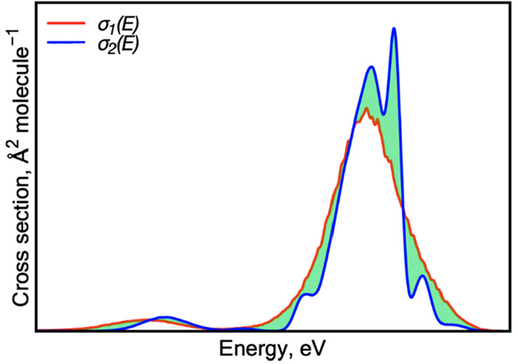
Integral (green) over absolute differences between two absorption cross sections σ1(E) (red) and σ2(E) (blue).
In this study, we use RIC to compare the ML cross section trained on Ntr points (ML-Ntr cross section σ2(E)) to the reference cross section σ1(E) (defined later). The same measure is then applied to compare pure TDDFT cross section obtained using only the training points (TD-Ntr cross section σ2(E)) to the cross section σ1(E). Thus, RIC allows us to compare the quality of the ML cross section obtained on the 50k-ensemble using the ML models trained on Ntr reference data and the pure TDDFT cross section obtained using the ensemble of Ntr points on equal footing. The phenomenological broadening of the spectrum of δ = 0.01 eV is used for all cross sections entering in eq 8 for consistency. The statistical error in the ML cross section stems mainly from ML inaccuracy, while the error in TDDFT cross section—from insufficient statistical sampling. Accuracy errors due to the quality of the TDDFT electronic structure and NEA approximations are out of the scope of this work and will not be discussed. The ML-NEA method proposed here does not aim at creating models transferable to other molecules, but rather to improve the existing NEA technique for a single system. Thus, an ML model must be trained for each new case.
The cross section calculations using our ML-NEA approach can be performed by following the online tutorial available at http://mlatom.com/tutorial/tutorial-mlnea. This tutorial also contains the necessary scripts (open source) and links to the required free software packages.
Computational Details
Absorption cross sections based on NEA were calculated with the Newton-X program package.45,46 Gaussian line shapes were used throughout. For benzene, we report new calculations done for this work, while for compound 2, we used the NEA spectrum from ref (47). In the case of benzene, the required geometry optimization and frequency calculations were performed at the B3LYP48/def2-TZVPP49−51 level of theory. TDDFT at the CAM-B3LYP52/ma-TZVP49−51,53 level of theory was used for calculating excitation energies and oscillator strengths. All electronic-structure calculations (geometry optimization, frequency, and excited-state calculations) for benzene were performed using the Gaussian 16 program package.54 See ref (47) for computational details for compound 2. The MLatom 1.1 program package38,55 was used for all ML calculations.
Results and Discussion
UV/vis absorption spectrum is often simulated convoluting the vertical excitations at the ground state minimum with Gaussian functions.2 While this single-point convolution approach may be useful as a first qualitative description of the spectrum, it fails to provide absolute band intensities and shapes. NEA cross sections, although still a low-level approach compared to precise spectrum simulations,3−5 significantly improve over that approximation. This improvement was clearly demonstrated on the example of benzene,7 where transitions into the first excited states are dipole-forbidden at the ground state geometry and only acquire some intensity via vibronic couplings. Thus, while the simple single-point convolution completely misses this low-energy feeble absorption band, NEA describes its envelope in good agreement with the experiments. However, to capture the envelope shape of this band precisely, a large ensemble (10k geometries) and their corresponding TDDFT calculations for the first four excited states were needed.
In this study, we recalculated the benzene cross section by using a five-times larger ensemble (50k-ensemble) for up to 10 excited states with the TD-CAM-B3LYP/ma-TZVP electronic structure method (data are available at 10.6084/m9.figshare.c.5081300). The TD-50k cross section is compared to the UV/vis spectrum calculated from a single-point convolution at the same level (Figure 2). This TDDFT method is close to the one used in the previous study; it gives a good agreement with experimental vertical excitations (Table 1). Due to the molecular symmetry, excitations into the first three excited states have zero oscillator strengths.
Figure 2.
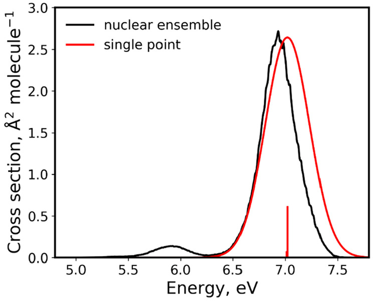
Comparison between the TD-50k absorption cross section of benzene obtained with NEA to a spectrum obtained from a single-point convolution at TD-CAM-B3LYP/ma-TZVP. Note the shift in the peak positions, the different width, and the complete absence of the low energy peak in the single-point convolution. TD-50k cross section was calculated for 50 thousand points in the ensemble and using broadening δ of 0.01 eV. The spectrum from single-point convolution was broadened using a Gaussian function with a width of 0.3 eV.
Table 1. TD-CAM-B3LYP/ma-TZVP Vertical Excitations of Benzene.
| TD-CAM-B3LYP/ma-TZVP | experimenta | |||
|---|---|---|---|---|
| ΔE, eV | f | ΔE, eV | assignment | |
| B2u | 5.47 | 0.000 | 4.90 | π–π* |
| B1u | 6.13 | 0.000 | 6.20 | π–π* |
| E1g | 6.53 | 0.000 | 6.33 | π–Ryd(s) |
| A2u | 7.01 | 0.066 | 6.93 | π–Ryd(pyz) |
| E1u | 7.02 | 0.608 | 6.94 | π–π* |
| E2u | 7.13 | 0.000 | 6.95 | π–Ryd(pyz) |
| A1u | 7.27 | 0.000 | N/A | π–Ryd(pyz) |
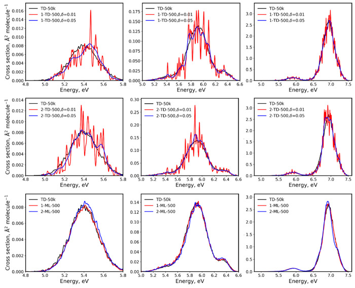
Using a small number of points in the ensemble leads to large errors due to insufficient statistical sampling in the case of pure TDDFT cross sections. Since the ensemble points are chosen stochastically, two cross sections generated independently with the same small number of ensemble points may be significantly different. For example, two TD-500 cross sections of benzene obtained with different 500-points ensembles show large statistical deviations between each other and with the reference TD-50k cross section, especially in the low-energy region (Figure 3, top and middle frames).
Figure 3.
Comparison of benzene absorption cross sections obtained with TDDFT and ML vs the TD-50k cross section. Two TDDFT cross sections (top frame, 1-TD-500; middle frame, 2-TD-500) were obtained with two 500-points ensembles and plotted for two values of phenomenological broadening δ = 0.01 and 0.05 eV. Two ML cross sections (1-ML-500 and 2-ML-500, bottom frame) were obtained with ML trained on 500 points and with 50k points in the ensemble. ML and TD-50k cross sections were plotted with δ = 0.01 eV. Left plots are plotted only for the first excitation, middle plots for the first three excitations, and the right plots for the entire spectrum considering 10 excitations. Note the different scales.
This number of points in the ensemble is large enough to be typically used in practical simulations and was used in the previous study for the entire spectrum of benzene.7 Nevertheless, it is clear from Figure 3 that this sampling is too sparse for calculating cross sections with a small phenomenological broadening of δ = 0.01 eV. That is why much larger δ values are typically used, e.g., in Newton-X the default value is 0.05 eV. However, while cross section with δ = 0.01 eV has too rough statistical fluctuations, cross section with δ = 0.05 eV broadens too much the low-energy region. Thus, this adjustment of δ is somewhat arbitrary. It is often done manually until the statistical fluctuations are smoothed out, trying not to affect the bandwidth. In the case of the low-energy region of benzene, simply adjusting δ is not sufficient, and one has to calculate cross section with many more ensemble points. In the previous study, 10k points were used as mentioned earlier.7
In contrast, ML cross sections are always generated for a vast number of points, and this practically eliminates errors due to insufficient statistical sampling. In addition, using ML for a large number of ensemble points naturally allows obtaining correct spectrum shape without the need to adjust the broadening parameter δ. Thus, we set δ to 0.01 eV for all ML cross sections (which, as discussed above, is much narrower than a typical bandwidth of ∼0.3 eV) and let the band be described entirely by the ensemble incoherent sum, making the NEA cross sections less parameter-dependent.
We trained ML on the corresponding sets of 500 points used for the above 1-TD-500 and 2-TD-500 cross sections and calculated the corresponding 1-ML-500 and 2-ML-500 cross sections of benzene. Both of these ML-500 cross sections look much more similar to the reference TD-50k than the TD-500 cross sections do (Figure 3). The ML-500 cross sections are also much more similar to each other compared to the TD-500 cross sections. In particular, the low-energy region is much better described by ML than by pure TDDFT. The reason behind it is that the contribution of a single strong outlier (e.g., some large oscillator strength for one state) to NEA cross section with a relatively small ensemble of 500 points can be significant, while for NEA cross section (both ML and TD) with a large ensemble of 50k points, the contribution of such an outlier is hundred times smaller as it is just one point out of 50k points. The computational cost of generating 50k points ML from 500 training points and 500 points TDDFT (or any other QC method) cross sections is virtually the same, as most of the computational time is spent in calculating excitation energies and oscillator strengths. In contrast, the cost of training ML models and making predictions with them is typically much lower.
Although using ML eliminates the error due to insufficient statistical sampling, it introduces another type of error due to inaccuracies of ML predictions (relative to the QC reference). These inaccuracies are generally smaller for larger training sets, but one wishes to use as small training set as possible to reduce the computational cost. Thus, as in the case of pure TDDFT cross section, we must find a trade-off between computational cost and cross section error. As we have seen from the above visual analysis, with the training set size equal to the typical number of points in a pure QC ensemble (500 points), ML cross sections can describe even the very challenging low-energy part of benzene spectrum. It is, however, interesting to systematically investigate how the quality of cross sections changes with an increasing number of training points. Performing visual analysis is too subjective, and that is why we employ the relative integral change (RIC) introduced in eq 8 as a quantitative error measure.
The dependence of RICs on the number of training points between 50k-ensemble ML cross sections and the reference TD-50k cross section (σ1(E) in eq 8) is shown in Figure 4. The figure also shows the RICs calculated for pure TDDFT cross sections obtained with an ensemble containing the same points as the corresponding ML training sets. In addition to the simple sequence of an increasing number of points, Figure 4 shows the mean value of the TDDFT and ML sequences calculated via bootstrapping using our 50k-ensemble benchmark. The error bars indicate one standard deviation around the mean value. As seen in the plots, ML RICs for benzene are generally lower than the RICs of TDDFT with the same number of points. The learning curve of ML RICs reaches small values of RIC (ca. 0.1 and below) much faster than the curve of TDDFT RICs.
Figure 4.
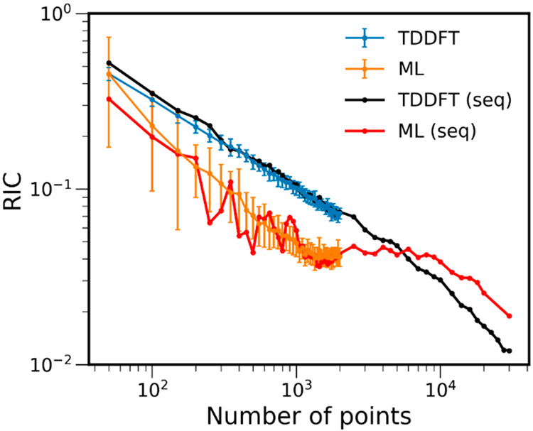
Relative integral change (RIC) of ML and TDDFT absorption cross sections of benzene calculated with an increasing number of points. The latter represents the size of the training set for a 50k-ensemble ML and the size of the ensemble for TDDFT. All RICs are calculated, taking the pure TDDFT cross section with 50k-ensemble (TD-50k) as the reference. Blue and orange curves are shown for mean RIC values obtained with dozens of calculations for each number of points (more than 100 for small training sets and ca. 30 and more for larger training sets), while black and red curves are shown for a single sequence of number of points (marked seq in the legend). The error bars are one standard deviation to the mean value. The plot is shown with log scaling. The RIC values and part of this plot in linear scaling are available at 10.6084/m9.figshare.c.5081300.
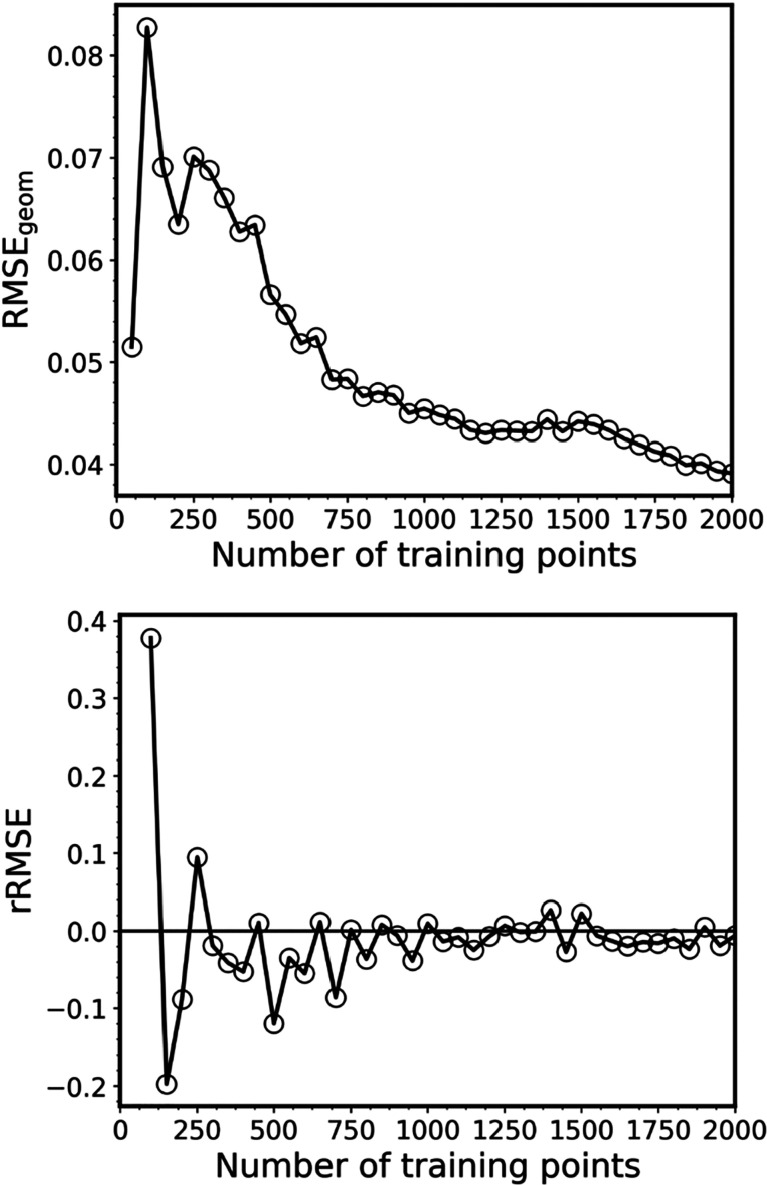
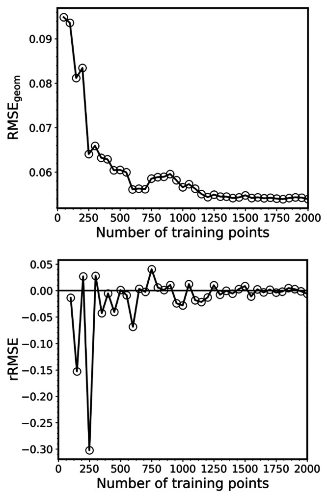
Of course, in practice, either with pure QC or ML methods, we usually do not have a reference cross section obtained with a large ensemble at the same level of theory, and therefore, RICs cannot be computed to estimate the errors. In the case of ML, we can, however, exploit the fact that the errors in the NEA cross section stem from ML inaccuracies. Based on that, we suggest to gauge the errors by looking at the geometric mean of the root-mean-square error (RMSEgeom) in the validation error of the ML models of all calculated properties, i.e., for each excitation energy and oscillator strength. It is also useful to look at how much the RMSEgeom changes with each additional batch of training points (here Nbatch = 50) added. Thus, here, we calculate the relative change of this error measure (rRMSE) as
| 9 |
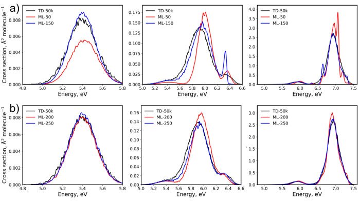
Converged ML models should have rRMSE close to zero. In Figure 5, we plot both RMSEgeom and rRMSE for one sequence of the training set sizes from 50 to 2k points (the sequence plotted in Figure 4). It shows that ML quickly converges, although the error decrease has oscillatory behavior with large jumps for small training sets. This behavior is consistent with the observation that the RIC standard deviations of ML cross sections quickly reduce, although they are rather large for small training sets (Figure 4). These large jumps in rRMSE indicate that the model is far from being converged, and we should treat such ML cross sections with caution. It is advised to generate the cross section when the rRMSE has only minimal oscillations for several consecutive training set sizes. Nevertheless, ML with relatively large RMSEgeom may give a qualitatively reasonable cross section. For example, even the ML-50 cross section trained on only 50 points from this particular sequence for benzene looks right for the low-energy region (Figure 6). As a rough threshold, one could use the rRMSE of less than 0.10 (preferably for several consecutive steps in the series of increasing training sets). In the case of benzene and this sequence, rRMSE drops below this threshold for training sets with 200 and more points. For example, ML-200 and ML-250 cross sections resemble closely the reference TD-50k cross section (Figure 6), and the RIC is practically the same for both ML-200 and TD-500 (both for this sequence and the mean RIC values, Figure 4). Remarkably, the ML-250 cross section from this sequence has very low RIC for the entire spectrum. RICs for ML with more than 500 training points are always smaller than that of TD-500, until the inversion point at 5k. This inversion point is caused by the fact that, in the limit of large ensembles and training sets, the error due to insufficient statistical sampling in case of TDDFT may become slightly smaller than the error due to the ML inaccuracies for the remaining points, because the reference is the TDDFT itself, while ML will always remain an approximation.
Figure 5.
Geometric mean of the root-mean-square error (RMSEgeom, top) and its relative change (rRMSE, bottom) in the validation error of the ML models for each of 10 excitation energies and oscillator strengths of benzene as the function of the training set size.
Figure 6.
ML absorption cross sections of benzene calculated with (a) 50 and 150 and (b) 200 and 250 training points compared to the reference TD-50k cross section.
The sampling of the low-energy band of benzene illustrates another potential use of our ML-NEA approach, to sample low-populated regions of the configurational space. For certain applications, like spectral band origin, tunneling,11 or dissociative electron attachment,58 we may need to generate ensembles with geometries that are rarely spanned in usual distributions. This situation implies that a massive number of QC calculations, often thousands, must be computed to find only a handful of adequate points. One of us has recently proposed an importance sampling method to enhance this special sampling in NEA.12 The method, however, requires the knowledge of the analytical form of the distribution, which is not always the case. With our ML-NEA model, after training the machine assuring the inclusion of a few rare points in the training set, we can generate as many new points as we want, to build an ensemble in the low-populated region.
As we have seen from the above discussion, benzene is an especially challenging molecule for absorption cross section simulations due to its dark low-energy excited states. It is, however, a small molecule for which methods much more advanced than NEA with TDDFT can be used. It is not the target of our ML approach, and it has been used here mostly for testing. Our main goal is to enable NEA for medium to large systems. Increasing the number of electrons and electronic states has a severe impact on the computational cost of each single point QC calculation in the ensemble. Conventional TDDFT algorithms, for instance, scale at least with the cube of the number of atoms.59 In contrast, the computational cost of generating ML cross section scales linearly with the number of considered excited states, and the cost increase remains mainly restricted to the number of reference QC calculations for the points in the training set.
In which follows, we test our approach on a medium-size molecule—an 9-dicyanomethylene derivative of acridine (2)—with 38 atoms (Chart 1). One of us has investigated the absorption spectrum of this compound earlier at the TD-ωB97XD60/def2-SVP49−51 level of theory by calculating NEA absorption cross section with 2000 points in the ensemble, considering energies and oscillator strengths for 30 excited states (data are available at 10.6084/m9.figshare.c.5081300).47 This TD-2k cross section agrees well with the experimental absorption spectrum.
Following the same procedure as discussed for benzene, we computed the NEA absorption cross section with the 50k-ensemble using ML models trained for one sequence with different training set sizes (we call it sequence 1). We first inspected the change in RMSEgeom and rRMSE with respect to the training set size. The trend shown in Figure 7 resembles that observed for benzene. We found out that ML practically converged with 2000 training points. Thus, we take the ML-2k cross section as the reference (σ1(E) in eq 8). Another indication that the 2k-ensemble is large enough to provide accurate results (relative to the QC reference) is that the RIC of the corresponding TD-2k cross section with respect to the ML-2k cross section is rather small, only 0.07.
Figure 7.
Geometric mean of the root-mean-square error (RMSEgeom, top) and its relative change (rRMSE, bottom) in the validation error of the ML models for each of 30 excitation energies and oscillator strengths of compound 2 as the function of the training set size.
The learning curves for RIC of both ML and TDDFT cross sections (Figure 8) are similar to that of benzene: ML reaches small values of RIC much faster than pure TDDFT cross sections. Considering the variability of the ML predictions, except for 50 and 100 points, the ML RIC is always smaller than the corresponding TDDFT RIC. The ML cross sections of compound 2 obtained with the smallest training set sizes have low quality (see, e.g., ML-50 for sequence 1 in Figure 9), but they quickly improve, showing an acceptable precision and accuracy level (RIC less than 0.1) already with 200 points (Figure 8). Interestingly, for the ML cross section trained with only 100 points in sequence 1, both RIC and rRMSE drop below the threshold of 0.1 (Figure 8 and Figure 7 bottom). Figure 9 also shows this ML cross section together with TDDFT cross sections. Because of the significant statistical errors in the small ensembles, the TDDFT cross sections were plotted with δ = 0.05 eV to smooth the oscillations. Even with this parameter adjustment, the TD-100 cross section shows many spurious maxima, while ML-100 in sequence 1 is free of them. Thus, ML allowed for obtaining cross sections of much better quality for this compound even with a much smaller number of points and without the need to adjust the δ parameter.
Figure 8.
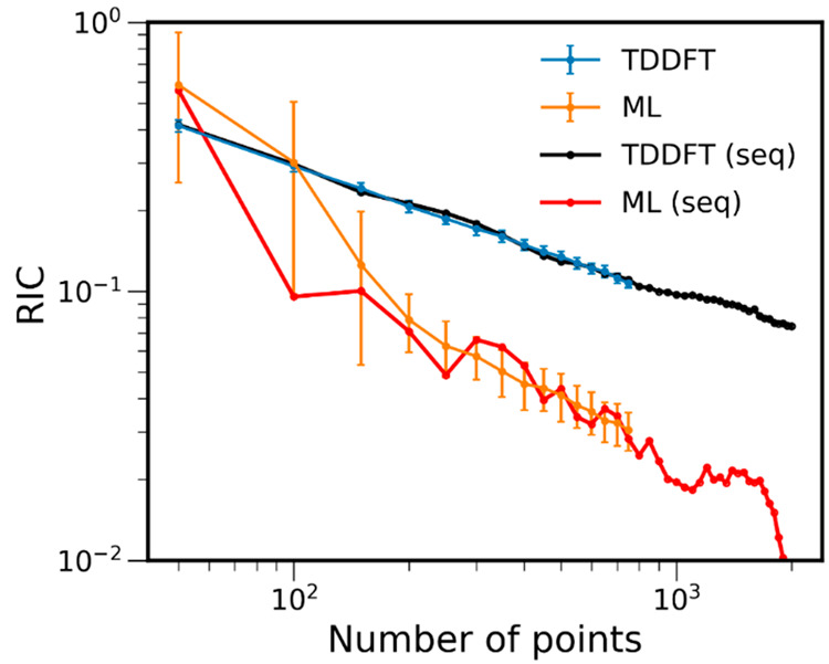
Relative integral change (RIC) of ML and TDDFT absorption cross sections of compound 2 calculated with an increasing number of points. The latter represents the size of the training set for ML and the size of the ensemble for TDDFT. ML-2k is taken as the reference cross section. Blue and orange curves are shown for mean RIC values obtained with dozens of calculations for each number of points (more than 100 for small training sets and ca. 30 and more for larger training sets), while black and red curves are shown for a single sequence of number of points (marked seq in the legend). The error bars are 1 standard deviation to the mean value. The plot is shown with log scaling. The RIC values and part of this plot in linear scaling are available at 10.6084/m9.figshare.c.5081300.
Figure 9.
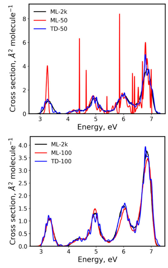
ML and TDDFT absorption cross sections of compound 2 calculated with 50 and 100 points compared to the ML-2k cross section as the reference. TDDFT cross sections were plotted with δ = 0.05 eV, while all other plots were generated with δ = 0.01 eV.
Satisfactory ML cross section for compound 2 can be obtained with fewer points than the cross section for the much smaller compound benzene. This fact shows that the complexity of the electronic structure (as the low-lying dark states of benzene) may play a more critical role in the simulation than the size of the molecule and the number of electronic excitations considered. The example for compound 2 also demonstrates that, with our ML approach, it is possible to refine existing cross sections generated only with a few hundred points, to obtain a high-quality ML cross section. The only additional computational cost incurred by ML stems from training ML models and making predictions with them. In the case of the KREG approach employed here, the training and making predictions with a single model for compound 2 on 1k points takes less than 12 s on Intel(R) Xeon(R) Gold 6240 CPU @ 2.60 GHz with 18 physical cores. With 30 states to calculate, 60 ML models are required, which amounts to only 12 min.
Conclusions
In this study, we developed a new ML approach to compute absorption cross sections within NEA. In this ML-NEA approach, a large ensemble with 50000 nuclear geometries is obtained by stochastically sampling a Wigner distribution for the quantum harmonic oscillator. The required electronic properties—excitation energies and oscillator strengths—are calculated only for a fraction of these points using the reference electronic structure method (here, we used linear-response TDDFT). The obtained data set is used as the training set for ML. We train individual ML models for each of the reference properties using the KREG model (KRR with the Gaussian kernel function and the RE descriptor) as implemented in MLatom to calculate the required properties for the remaining points in the large ensemble. The combined set of reference and ML properties is used to calculate the NEA cross section as implemented in Newton-X.
We also suggest using the ML validation-set errors to gauge the convergence of the ML-NEA model. It provides a criterion for defining the required number of reference data calculated with electronic structure methods. Such a criterion is convenient for calculating NEA cross sections of new molecules when it is not clear how many electronic structure calculations should be performed to obtain satisfactory accuracy and precision. Our approach also allows refining cross sections calculated earlier with relatively small ensembles without incurring substantial additional cost.
We demonstrated how the ML-NEA approach and the accuracy criterion can successfully predict absorption cross sections by applying them to two examples, benzene (1) and an 9-dicyanomethylene derivative of acridine (2) (Chart 1).
Our ML-NEA approach brings the following benefits:
It allows obtaining high precision and high accuracy NEA cross sections for small to medium-size molecules at the cost of a few hundreds of single-point QC calculations. To achieve the same quality of pure QC-NEA cross sections would require tens of thousands of QC calculations.
It eliminates the need to use the line-shape arbitrary broadening parameter δ to smooth the NEA cross section. This parameter is fixed to a tiny constant value that does not impact the final result.
We anticipate that our ML-NEA approach may routinely allow obtaining NEA absorption cross sections for medium to large size molecules with reasonable accuracy and high precision at the cost of about one hundred QC single points. It may also allow sampling regions of the configurational space with a low population at the cost of a few hundred QC calculations.
We note that the error of ML cross sections built with hundreds of training points relative to the reference cross sections built with thousands of points in the ensemble is much smaller than the error introduced by approximations in QC methods and NEA itself. Our best theoretical cross sections used as the reference (TD-50k cross section for benzene and ML-2k cross section for compound 2) deviate much stronger from available experimental absorption cross sections, than the ML cross sections trained on hundreds of points deviate from the theoretical reference (Figure 10). The RICs between our best reference theoretical and experimental cross sections are also much larger: 0.31 and 1.39 for benzene and compound 2, respectively, while RICs of ML-250 (benzene) and ML-100 (compound 2) are 0.06–0.07 relative to the corresponding best reference theoretical cross sections. Our ML approach allows reducing substantially the number of QC calculations, which, in turn, allows using higher level (and more costly) QC methods for training, improving the accuracy of the theoretical cross sections.
Figure 10.
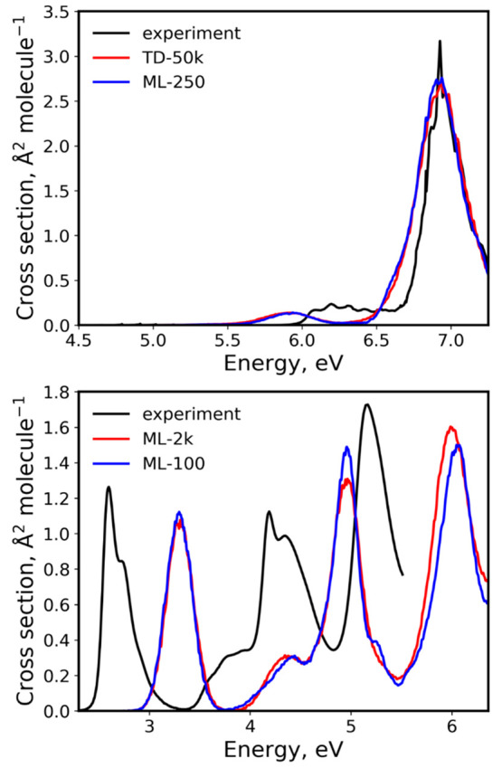
Best theoretical cross sections in this work (TD-50k for benzene and ML-2k for compound 2) vs the experimental cross sections (taken from ref (56) for benzene and ref (47) for compound 2). For comparison, ML-250 cross section for benzene and ML-100 cross section for compound 2 are also plotted. The experimental cross section for benzene was recorded in the gas phase, while for compound 2 it was recorded in CH2Cl2. The quantum chemical method used for benzene was TD-CAM-B3LYP/ma-TZVP, and for compound 2, it was TD-ωB97XD/def2-SVP, with all calculations performed in vacuum. Top: benzene. Bottom: compound 2.
We tested our ML-NEA model for absorption spectra based on Wigner distributions and TDDFT electronic structure. Nevertheless, this approach is much more general. It can be used for other types of NEA spectra (like emission,7 two-dimensional,61 differential transmission,62 photoelectron,63 ultrafast Auger,64 and X-ray photoscattering65 spectroscopies), with any ensemble distribution (e.g., from molecular dynamics20) and any QC method able to compute excitation energies and transition moments.
Glossary
Abbreviations
- ML
machine learning
- DFT
density functional theory
- TDDFT
time-dependent density functional theory
- NEA
nuclear-ensemble approach
Author Contributions
The manuscript was written through contributions of all authors. All authors have given approval to the final version of the manuscript.
M.B. expresses thanks for the support of the European Research Council (ERC) Advanced Grant SubNano (Grant Agreement 832237). P.O.D. acknowledges funding via the Lab project of the State Key Laboratory of Physical Chemistry of Solid Surfaces.
The authors declare no competing financial interest.
Notes
Data Availability. Hyperparameter values for ML models, RIC, RMSEgeom, and rRMSE values used to plot Figures 4, 5, 7, and 8, parts of Figures 4 and 8 in linear scaling, and the data sets used in this study containing geometries in xyz format and reference TDDFT values for each excitation energy and oscillator strength of benzene and compound 2 are openly available in figshare at 10.6084/m9.figshare.c.5081300.
Special Issue
Published as part of The Journal of Physical Chemistry virtual special issue “Machine Learning in Physical Chemistry”.
References
- Hachmann J.; Olivares-Amaya R.; Atahan-Evrenk S.; Amador-Bedolla C.; Sánchez-Carrera R. S.; Gold-Parker A.; Vogt L.; Brockway A. M.; Aspuru-Guzik A. The Harvard Clean Energy Project: Large-Scale Computational Screening and Design of Organic Photovoltaics on the World Community Grid. J. Phys. Chem. Lett. 2011, 2, 2241–2251. 10.1021/jz200866s. [DOI] [Google Scholar]
- Bai S.; Mansour R.; Stojanovic L.; Toldo J. M.; Barbatti M. On the origin of the shift between vertical excitation and band maximum in molecular photoabsorption. J. Mol. Model. 2020, 26, 107. 10.1007/s00894-020-04355-y. [DOI] [PMC free article] [PubMed] [Google Scholar]
- Petrenko T.; Neese F. Analysis and prediction of absorption band shapes, fluorescence band shapes, resonance Raman intensities, and excitation profiles using the time-dependent theory of electronic spectroscopy. J. Chem. Phys. 2007, 127, 164319. 10.1063/1.2770706. [DOI] [PubMed] [Google Scholar]
- Reddy C. S.; Prasad M. D. A Gaussian Wave Packet Propagation Approach to Vibrationally Resolved Optical Spectra at Non-Zero Temperatures. J. Phys. Chem. A 2016, 120, 2583–2590. 10.1021/acs.jpca.6b00308. [DOI] [PubMed] [Google Scholar]
- Barone V.Computational strategies for spectroscopy: from small molecules to nano systems; John Wiley & Sons: 2011. [Google Scholar]
- Lischka H.; Nachtigallova D.; Aquino A. J. A.; Szalay P. G.; Plasser F.; Machado F. B. C.; Barbatti M. Multireference Approaches for Excited States of Molecules. Chem. Rev. 2018, 118, 7293–7361. 10.1021/acs.chemrev.8b00244. [DOI] [PubMed] [Google Scholar]
- Crespo-Otero R.; Barbatti M. Spectrum simulation and decomposition with nuclear ensemble: formal derivation and application to benzene, furan and 2-phenylfuran. Theor. Chem. Acc. 2012, 131, 1237. 10.1007/s00214-012-1237-4. [DOI] [Google Scholar]
- Dreuw A.; Head-Gordon M. Single-Reference ab Initio Methods for the Calculation of Excited States of Large Molecules. Chem. Rev. 2005, 105, 4009–4037. 10.1021/cr0505627. [DOI] [PubMed] [Google Scholar]
- Crespo-Otero R.; Barbatti M. Recent Advances and Perspectives on Nonadiabatic Mixed Quantum-Classical Dynamics. Chem. Rev. 2018, 118, 7026–7068. 10.1021/acs.chemrev.7b00577. [DOI] [PubMed] [Google Scholar]
- Suchan J.; Hollas D.; Curchod B. F. E.; Slavíček P. On the importance of initial conditions for excited-state dynamics. Faraday Discuss. 2018, 212, 307–330. 10.1039/C8FD00088C. [DOI] [PubMed] [Google Scholar]
- Zheng J.; Xu X.; Meana-Pañeda R.; Truhlar D. G. Army ants tunneling for classical simulations. Chem. Sci. 2014, 5, 2091–2099. 10.1039/C3SC53290A. [DOI] [Google Scholar]
- Kossoski F.; Barbatti M. Nuclear Ensemble Approach with Importance Sampling. J. Chem. Theory Comput. 2018, 14, 3173–3183. 10.1021/acs.jctc.8b00059. [DOI] [PubMed] [Google Scholar]
- Dral P. O. Quantum Chemistry in the Age of Machine Learning. J. Phys. Chem. Lett. 2020, 11, 2336–2347. 10.1021/acs.jpclett.9b03664. [DOI] [PubMed] [Google Scholar]
- von Lilienfeld O. A. Quantum Machine Learning in Chemical Compound Space. Angew. Chem., Int. Ed. 2018, 57, 4164–4169. 10.1002/anie.201709686. [DOI] [PubMed] [Google Scholar]
- Dral P. O.Quantum Chemistry Assisted by Machine Learning. In Advances in Quantum Chemistry: Chemical Physics and Quantum Chemistry, 1st ed.; Brandas E., Ruud K., Eds. Academic Press, 2020, Vol. 81, In Press. 10.1016/bs.aiq.2020.05.002 [DOI] [Google Scholar]
- Nantasenamat C.; Isarankura-Na-Ayudhya C.; Tansila N.; Naenna T.; Prachayasittikul V. Prediction of GFP spectral properties using artificial neural network. J. Comput. Chem. 2007, 28, 1275–1289. 10.1002/jcc.20656. [DOI] [PubMed] [Google Scholar]
- Wang J. N.; Jin J. L.; Geng Y.; Sun S. L.; Xu H. L.; Lu Y. H.; Su Z. M. An accurate and efficient method to predict the electronic excitation energies of BODIPY fluorescent dyes. J. Comput. Chem. 2013, 34, 566–575. 10.1002/jcc.23168. [DOI] [PubMed] [Google Scholar]
- Ramakrishnan R.; Hartmann M.; Tapavicza E.; von Lilienfeld O. A. Electronic spectra from TDDFT and machine learning in chemical space. J. Chem. Phys. 2015, 143, 084111. 10.1063/1.4928757. [DOI] [PubMed] [Google Scholar]
- Hu D.; Xie Y.; Li X.; Li L.; Lan Z. Inclusion of Machine Learning Kernel Ridge Regression Potential Energy Surfaces in On-the-Fly Nonadiabatic Molecular Dynamics Simulation. J. Phys. Chem. Lett. 2018, 9, 2725–2732. 10.1021/acs.jpclett.8b00684. [DOI] [PubMed] [Google Scholar]
- Ye S.; Hu W.; Li X.; Zhang J.; Zhong K.; Zhang G.; Luo Y.; Mukamel S.; Jiang J. A neural network protocol for electronic excitations of N-methylacetamide. Proc. Natl. Acad. Sci. U. S. A. 2019, 116, 11612–11617. 10.1073/pnas.1821044116. [DOI] [PMC free article] [PubMed] [Google Scholar]
- Dral P. O.; Barbatti M.; Thiel W. Nonadiabatic Excited-State Dynamics with Machine Learning. J. Phys. Chem. Lett. 2018, 9, 5660–5663. 10.1021/acs.jpclett.8b02469. [DOI] [PMC free article] [PubMed] [Google Scholar]
- Chen W.-K.; Liu X.-Y.; Fang W.; Dral P. O.; Cui G. Deep Learning for Nonadiabatic Excited-State Dynamics. J. Phys. Chem. Lett. 2018, 9, 6702–6708. 10.1021/acs.jpclett.8b03026. [DOI] [PubMed] [Google Scholar]
- da Silva R. S.; Marins L. F.; Almeida D. V.; Dos Santos Machado K.; Werhli A. V. A comparison of classifiers for predicting the class color of fluorescent proteins. Comput. Biol. Chem. 2019, 83, 107089. 10.1016/j.compbiolchem.2019.107089. [DOI] [PubMed] [Google Scholar]
- Ghosh K.; Stuke A.; Todorovic M.; Jorgensen P. B.; Schmidt M. N.; Vehtari A.; Rinke P. Deep Learning Spectroscopy: Neural Networks for Molecular Excitation Spectra. Adv. Sci. 2019, 6, 1801367. 10.1002/advs.201801367. [DOI] [PMC free article] [PubMed] [Google Scholar]
- Westermayr J.; Gastegger M.; Menger M. F. S. J.; Mai S.; González L.; Marquetand P. Machine learning enables long time scale molecular photodynamics simulations. Chem. Sci. 2019, 10, 8100–8107. 10.1039/C9SC01742A. [DOI] [PMC free article] [PubMed] [Google Scholar]
- Westermayr J.; Gastegger M.; Marquetand P. Combining SchNet and SHARC: The SchNarc Machine Learning Approach for Excited-State Dynamics. J. Phys. Chem. Lett. 2020, 11, 3828–3834. 10.1021/acs.jpclett.0c00527. [DOI] [PMC free article] [PubMed] [Google Scholar]
- Westermayr J.; Faber F. A.; Christensen A. S.; von Lilienfeld O. A.; Marquetand P. Neural networks and kernel ridge regression for excited states dynamics of CH2NH2+: From single-state to multi-state representations and multi-property machine learning models. Mach. Learn.: Sci. Technol. 2020, 1, 025009. 10.1088/2632-2153/ab88d0. [DOI] [Google Scholar]
- Chen M. S.; Zuehlsdorff T. J.; Morawietz T.; Isborn C. M.; Markland T. E. Exploiting machine learning to efficiently predict multidimensional optical spectra in complex environments. J. Phys. Chem. Lett. 2020, 10.1021/acs.jpclett.0c02168. [DOI] [PubMed] [Google Scholar]
- Wu Z.; Ramsundar B.; Feinberg E. N.; Gomes J.; Geniesse C.; Pappu A. S.; Leswing K.; Pande V. MoleculeNet: a benchmark for molecular machine learning. Chem. Sci. 2018, 9, 513–530. 10.1039/C7SC02664A. [DOI] [PMC free article] [PubMed] [Google Scholar]
- Pronobis W.; Schütt K. T.; Tkatchenko A.; Müller K.-R. Capturing intensive and extensive DFT/TDDFT molecular properties with machine learning. Eur. Phys. J. B 2018, 91, 178. 10.1140/epjb/e2018-90148-y. [DOI] [Google Scholar]
- Häse F.; Valleau S.; Pyzer-Knapp E.; Aspuru-Guzik A. Machine learning exciton dynamics. Chem. Sci. 2016, 7, 5139–5147. 10.1039/C5SC04786B. [DOI] [PMC free article] [PubMed] [Google Scholar]
- Richings G. W.; Habershon S. Direct grid-based quantum dynamics on propagated diabatic potential energy surfaces. Chem. Phys. Lett. 2017, 683, 228–233. 10.1016/j.cplett.2017.01.063. [DOI] [Google Scholar]
- Richings G. W.; Habershon S. Direct Quantum Dynamics Using Grid-Based Wave Function Propagation and Machine-Learned Potential Energy Surfaces. J. Chem. Theory Comput. 2017, 13, 4012–4024. 10.1021/acs.jctc.7b00507. [DOI] [PubMed] [Google Scholar]
- Häse F.; Kreisbeck C.; Aspuru-Guzik A. Machine learning for quantum dynamics: deep learning of excitation energy transfer properties. Chem. Sci. 2017, 8, 8419–8426. 10.1039/C7SC03542J. [DOI] [PMC free article] [PubMed] [Google Scholar]
- Nantasenamat C.; Srungboonmee K.; Jamsak S.; Tansila N.; Isarankura-Na-Ayudhya C.; Prachayasittikul V. Quantitative structure-property relationship study of spectral properties of green fluorescent protein with support vector machine. Chemom. Intell. Lab. Syst. 2013, 120, 42–52. 10.1016/j.chemolab.2012.11.003. [DOI] [Google Scholar]
- Rankine C. D.; Madkhali M. M. M.; Penfold T. J. A Deep Neural Network for the Rapid Prediction of X-ray Absorption Spectra. J. Phys. Chem. A 2020, 124, 4263–4270. 10.1021/acs.jpca.0c03723. [DOI] [PubMed] [Google Scholar]
- Smith J. S.; Isayev O.; Roitberg A. E. ANI-1: an extensible neural network potential with DFT accuracy at force field computational cost. Chem. Sci. 2017, 8, 3192–3203. 10.1039/C6SC05720A. [DOI] [PMC free article] [PubMed] [Google Scholar]
- Dral P. O. MLatom: A Program Package for Quantum Chemical Research Assisted by Machine Learning. J. Comput. Chem. 2019, 40, 2339–2347. 10.1002/jcc.26004. [DOI] [PubMed] [Google Scholar]
- Dral P. O.; Owens A.; Yurchenko S. N.; Thiel W. Structure-based sampling and self-correcting machine learning for accurate calculations of potential energy surfaces and vibrational levels. J. Chem. Phys. 2017, 146, 244108. 10.1063/1.4989536. [DOI] [PubMed] [Google Scholar]
- Barbatti M.; Sen K. Effects of Different Initial Condition Samplings on Photodynamics and Spectrum of Pyrrole. Int. J. Quantum Chem. 2016, 116, 762–771. 10.1002/qua.25049. [DOI] [Google Scholar]
- Ruckenbauer M.; Barbatti M.; Muller T.; Lischka H. Nonadiabatic excited-state dynamics with hybrid ab initio quantum-mechanical/molecular-mechanical methods: solvation of the pentadieniminium cation in apolar media. J. Phys. Chem. A 2010, 114, 6757–6765. 10.1021/jp103101t. [DOI] [PubMed] [Google Scholar]
- Schinke R.Photodissociation Dynamics: Spectroscopy and Fragmentation of Small Polyatomic Molecules; Cambridge University Press: Cambridge, U.K., 1995. [Google Scholar]
- Dral P. O.; Owens A.; Dral A.; Csányi G. Hierarchical Machine Learning of Potential Energy Surfaces. J. Chem. Phys. 2020, 152, 204110. 10.1063/5.0006498. [DOI] [PubMed] [Google Scholar]
- Rasmussen C. E.; Williams C. K. I.. Gaussian Processes for Machine Learning; The MIT Press: Boston, MA, 2006. [Google Scholar]
- Barbatti M.; Ruckenbauer M.; Plasser F.; Pittner J.; Granucci G.; Persico M.; Lischka H. Newton-X: a surface-hopping program for nonadiabatic molecular dynamics. WIREs: Comp. Mol. Sci. 2014, 4, 26–33. 10.1002/wcms.1158. [DOI] [Google Scholar]
- Barbatti M.; Granucci G.; Ruckenbauer M.; Plasser F.; Crespo-Otero R.; Pittner J.; Persico M.; Lischka H.. NEWTON-X: a package for Newtonian dynamics close to the crossing seam; www.newtonx.org.
- Schaub T. A.; Brülls S. M.; Dral P. O.; Hampel F.; Maid H.; Kivala M. Organic Electron Acceptors Comprising a Dicyanomethylene-Bridged Acridophosphine Scaffold: The Impact of the Heteroatom. Chem. - Eur. J. 2017, 23, 6988–6992. 10.1002/chem.201701412. [DOI] [PubMed] [Google Scholar]
- Becke A. D. A New Mixing of Hartree-Fock and Local Density-Functional Theories. J. Chem. Phys. 1993, 98, 1372–1377. 10.1063/1.464304. [DOI] [Google Scholar]
- Weigend F.; Ahlrichs R. Balanced basis sets of split valence, triple zeta valence and quadruple zeta valence quality for H to Rn: Design and assessment of accuracy. Phys. Chem. Chem. Phys. 2005, 7, 3297–3305. 10.1039/b508541a. [DOI] [PubMed] [Google Scholar]
- Schäfer A.; Huber C.; Ahlrichs R. Fully optimized contracted Gaussian-basis sets of triple zeta valence quality for atoms Li to Kr. J. Chem. Phys. 1994, 100, 5829–5835. 10.1063/1.467146. [DOI] [Google Scholar]
- Schäfer A.; Horn H.; Ahlrichs R. Fully Optimized Contracted Gaussian-Basis Sets for Atoms Li to Kr. J. Chem. Phys. 1992, 97, 2571–2577. 10.1063/1.463096. [DOI] [Google Scholar]
- Yanai T.; Tew D. P.; Handy N. C. A new hybrid exchange-correlation functional using the Coulomb-attenuating method (CAM-B3LYP). Chem. Phys. Lett. 2004, 393, 51–57. 10.1016/j.cplett.2004.06.011. [DOI] [Google Scholar]
- Zheng J.; Xu X.; Truhlar D. G. Minimally augmented Karlsruhe basis sets. Theor. Chem. Acc. 2011, 128, 295–305. 10.1007/s00214-010-0846-z. [DOI] [Google Scholar]
- Frisch M. J.; Trucks G. W.; Schlegel H. B.; Scuseria G. E.; Robb M. A.; Cheeseman J. R.; Scalmani G.; Barone V.; Petersson G. A.; Nakatsuji H.; Li X.; Caricato M.; Marenich A. V.; Bloino J.; Janesko B. G.; Gomperts R.; Mennucci B.; Hratchian H. P.; Ortiz J. V.; Izmaylov A. F.; Sonnenberg J. L.; Williams; Ding F.; Lipparini F.; Egidi F.; Goings J.; Peng B.; Petrone A.; Henderson T.; Ranasinghe D.; Zakrzewski V. G.; Gao J.; Rega N.; Zheng G.; Liang W.; Hada M.; Ehara M.; Toyota K.; Fukuda R.; Hasegawa J.; Ishida M.; Nakajima T.; Honda Y.; Kitao O.; Nakai H.; Vreven T.; Throssell K.; Montgomery J. A. Jr.; Peralta J. E.; Ogliaro F.; Bearpark M. J.; Heyd J. J.; Brothers E. N.; Kudin K. N.; Staroverov V. N.; Keith T. A.; Kobayashi R.; Normand J.; Raghavachari K.; Rendell A. P.; Burant J. C.; Iyengar S. S.; Tomasi J.; Cossi M.; Millam J. M.; Klene M.; Adamo C.; Cammi R.; Ochterski J. W.; Martin R. L.; Morokuma K.; Farkas O.; Foresman J. B.; Fox D. J.. Gaussian 16, Rev. C.01; Wallingford, CT, 2016. [Google Scholar]
- Dral P. O.MLatom: A Package for Atomistic Simulations with Machine Learning, ver. 1.1; Xiamen University; Xiamen, China, http://MLatom.com (accessed June 10, 2020), 2013–2020. [Google Scholar]
- Bolovinos A.; Philis J.; Pantos E.; Tsekeris P.; Andritsopoulos G. The methylbenzenes vis-à-vis benzene. J. Mol. Spectrosc. 1982, 94, 55–68. 10.1016/0022-2852(82)90293-4. [DOI] [Google Scholar]
- Li Y.; Wan J.; Xu X. Theoretical study of the vertical excited states of benzene, pyrimidine, and pyrazine by the symmetry adapted cluster--configuration interaction method. J. Comput. Chem. 2007, 28, 1658–1667. 10.1002/jcc.20555. [DOI] [PubMed] [Google Scholar]
- Kossoski F.; Varella M.; Barbatti M. On-the-fly dynamics simulations of transient anions. J. Chem. Phys. 2019, 151, 224104. 10.1063/1.5130547. [DOI] [PubMed] [Google Scholar]
- Zuehlsdorff T. J.; Hine N. D.; Payne M. C.; Haynes P. D. Linear-scaling time-dependent density-functional theory beyond the Tamm-Dancoff approximation: Obtaining efficiency and accuracy with in situ optimised local orbitals. J. Chem. Phys. 2015, 143, 204107. 10.1063/1.4936280. [DOI] [PubMed] [Google Scholar]
- Chai J.-D.; Head-Gordon M. Long-range corrected hybrid density functionals with damped atom-atom dispersion corrections. Phys. Chem. Chem. Phys. 2008, 10, 6615–6620. 10.1039/b810189b. [DOI] [PubMed] [Google Scholar]
- Segarra-Martí J.; Segatta F.; Mackenzie T. A.; Nenov A.; Rivalta I.; Bearpark M. J.; Garavelli M. Modeling multidimensional spectral lineshapes from first principles: application to water-solvated adenine. Faraday Discuss. 2020, 221, 219–244. 10.1039/C9FD00072K. [DOI] [PubMed] [Google Scholar]
- Polli D.; Altoe P.; Weingart O.; Spillane K. M.; Manzoni C.; Brida D.; Tomasello G.; Orlandi G.; Kukura P.; Mathies R. A.; Garavelli M.; Cerullo G. Conical Intersection Dynamics of the Primary Photoisomerization Event in Vision. Nature 2010, 467, 440–443. 10.1038/nature09346. [DOI] [PubMed] [Google Scholar]
- Arbelo-González W.; Crespo-Otero R.; Barbatti M. Steady and Time-Resolved Photoelectron Spectra Based on Nuclear Ensembles. J. Chem. Theory Comput. 2016, 12, 5037–5049. 10.1021/acs.jctc.6b00704. [DOI] [PubMed] [Google Scholar]
- McFarland B. K.; Farrell J. P.; Miyabe S.; Tarantelli F.; Aguilar A.; Berrah N.; Bostedt C.; Bozek J. D.; Bucksbaum P. H.; Castagna J. C.; Coffee R. N.; Cryan J. P.; Fang L.; Feifel R.; Gaffney K. J.; Glownia J. M.; Martinez T. J.; Mucke M.; Murphy B.; Natan A.; Osipov T.; Petrović V. S.; Schorb S.; Schultz T.; Spector L. S.; Swiggers M.; Tenney I.; Wang S.; White J. L.; White W.; Gühr M. Ultrafast X-Ray Auger Probing of Photoexcited Molecular Dynamics. Nat. Commun. 2014, 5, 4235. 10.1038/ncomms5235. [DOI] [PubMed] [Google Scholar]
- Bennett K.; Kowalewski M.; Mukamel S. Probing Electronic and Vibrational Dynamics in Molecules by Time-Resolved Photoelectron, Auger-Electron, and X-Ray Photon Scattering Spectroscopy. Faraday Discuss. 2015, 177, 405–428. 10.1039/C4FD00178H. [DOI] [PMC free article] [PubMed] [Google Scholar]


