Abstract
The SIR (‘susceptible-infectious-recovered’) formulation is used to uncover the generic spread mechanisms observed by COVID-19 dynamics globally, especially in the early phases of infectious spread. During this early period, potential controls were not effectively put in place or enforced in many countries. Hence, the early phases of COVID-19 spread in countries where controls were weak offer a unique perspective on the ensemble-behavior of COVID-19 basic reproduction number Ro inferred from SIR formulation. The work here shows that there is global convergence (i.e., across many nations) to an uncontrolled Ro = 4.5 that describes the early time spread of COVID-19. This value is in agreement with independent estimates from other sources reviewed here and adds to the growing consensus that the early estimate of Ro = 2.2 adopted by the World Health Organization is low. A reconciliation between power-law and exponential growth predictions is also featured within the confines of the SIR formulation. The effects of testing ramp-up and the role of ‘super-spreaders’ on the inference of Ro are analyzed using idealized scenarios. Implications for evaluating potential control strategies from this uncontrolled Ro are briefly discussed in the context of the maximum possible infected fraction of the population (needed to assess health care capacity) and mortality (especially in the USA given diverging projections). Model results indicate that if intervention measures still result in Ro > 2.7 within 44 days after first infection, intervention is unlikely to be effective in general for COVID-19.
Introduction
A heated dispute about the effectiveness versus risk of smallpox inoculation was playing out in eighteenth-century France, which was to launch the use of mathematical models in epidemiology. This dispute moved inoculation from the domain of philosophy, religion, and disjointed trials plagued by high uncertainty into a debate about mathematical models—put forth by Daniel Bernoulli (in 1766) and Jean-Baptiste le Rond D’Alembert (in 1761), both dealing with competing risks of death and interpretation of trials [1]. Since then, the mathematical description of infectious diseases continues to draw significant attention from researchers and practitioners in governments and health agencies alike. Even news agencies are now seeking out explanations to models so as to offer advice and clarity to their audiences during the (near-continuous) coverage of the spread of COVID-19 [2]. The prospect of using mathematical models in conjunction with data is succinctly summarized by the Nobel laureate Ronald Ross, whose 1916 abstract [3] continues to enlighten the role of mathematics in epidemiology today. A quotation from this abstract below, which foreshadows the requirements and challenges for mathematical models to describe emerging epidemics such as COVID-19 [4, 5], needs no further elaboration:
It is somewhat surprising that so little mathematical work should have been done on the subject of epidemics, and, indeed, on the distribution of diseases in general. Not only is the theme of immediate importance to humanity, but it is one which is fundamentally connected with numbers, while vast masses of statistics have long been awaiting proper examination. But, more than this, many and indeed the principal problems of epidemiology on which preventive measures largely depend, such as the rate of infection, the frequency of outbreaks, and the loss of immunity, can scarcely ever be resolved by any other methods than those of mathematical analysis.
The classic susceptible-infectious-recovered (SIR) paradigm, initiated in the late 1920s [6], now provides a mathematical framework that describes the core transmission dynamics of a wide range of human diseases [7–12], including COVID-19 [13]. A key parameter in the SIR paradigm is the basic reproduction number (Ro). The Ro is defined by the average number of secondary cases arising from a typical primary case in an entirely susceptible population of size So [14– 16]. The usefulness of Ro and uncertainty in its estimation are not a subject of debate, as reviewed elsewhere [17], and therefore are not further discussed here.
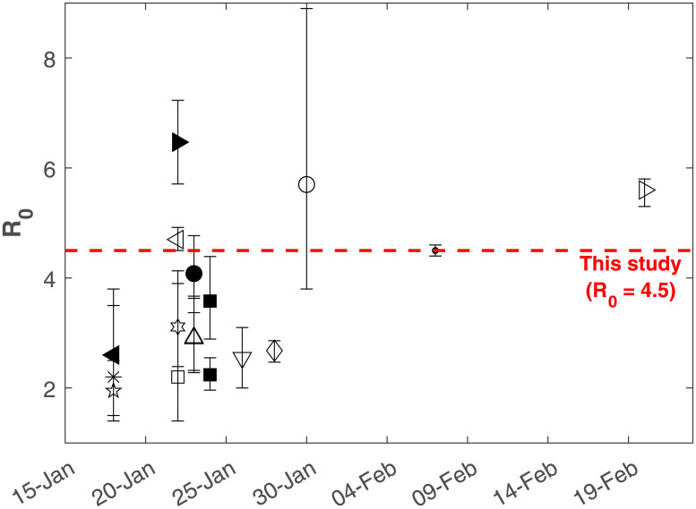
The Ro for COVID-19 and other diseases is commonly estimated directly from case data or by fitting the SIR model or one of its many variants to the data [14, 18–22]. Unsurprisingly, the Ro estimates often exhibit large uncertainty. For COVID-19, mean estimated Ro ranges between 1.95 and 6.47, with corresponding error estimates giving upper and lower bounds of 1.4 and 8.9 (Fig 1). For a given virus, such variability in Ro is attributed to local spatio-temporal variability in public health resources, interventions, and how individuals in a population interact, among others, as well as the estimation method used [15, 17]. Due to this local variability, it is commonly held that Ro is a site-specific parameter that cannot be directly transferred between sites. The rapid availability of global data for COVID-19 has allowed an unprecedented comparison across a diverse array of populations, which is absent from the prior literature on Ro estimation.
Fig 1. Timeline of the COVID-19 Ro estimates.
Symbols represent studies listed in Appendix (Table 1) while the red dashed line marks Ro = 4.5 derived from this study. An initial Ro = 2.2 was initially adopted by the World Health Organization (WHO).
In the analysis herein, the SIR model is used to uncover generic spread mechanisms observed by COVID-19 dynamics globally, especially in the early phases of infectious spread. During this early period, potential controls were not effectively put in place or enforced in many countries around the world despite early warning signals from China, Iran, and later on, Italy. Hence, the early phases of COVID-19 spread in many countries where controls were weak offer a unique perspective on the ensemble-behavior of COVID-19 Ro. The analysis shows that there is global convergence (i.e. across many nations) to an uncontrolled Ro = 4.5 for COVID-19 describing early times spread from the SIR model. This value is compared to a number of published Ro estimates for COVID-19 with a timeline summary featured in Fig 1. These published estimates along with the methods used to infer Ro, the published uncertainty, and the original data source are provided in the Appendix.
Clearly, such wide ranging values of Ro in Fig 1 motivate further analysis of Ro variability across populations, the objective of this analysis. Other aspects that are considered in the estimation of Ro from SIR are the effects of ramp-up in testing at the early phases of disease spread and the role of super-spreaders. These two effects are briefly discussed using idealized scenarios and model calculations. The implications for evaluating potential control strategies from this uncontrolled Ro are considered in the context of mortality and maximum infections.
Theory
Definitions and nomenclature
Mathematical models of disease spread assume that a population within a compartment (e.g., city, region, country) can be subdivided into a set of distinct classes [11]. The SIR model classifies individuals in the compartment as one of three classes: susceptible (S), infectious (I), and recovered or removed (R). Infectious individuals spread the disease to susceptible individuals and remain in the infectious class for a given period of time known as the infectious period before moving into the recovered (or removed) class. Individuals in the recovered class are assumed to be immune for an extended period (or removed from the population). For the total population N = S + I + R, the dynamical system describing the SIR equations are given as
| (1) |
| (2) |
| (3) |
where β(I/N) is known as the force of infection and coefficients β and γ must be externally supplied. Moreover, this system requires the specification of three initial conditions at time t = 0, S(0), I(0), and R(0). For COVID-19, it is assumed that R(0) = 0 and I(0)≪S(0) at the initial outbreak. For the initial conditions selected here, N = S(0) + I(0) + R(0) ≈ S(0), which is labeled So for notational simplicity and consistency with the SIR literature. The basis of the latter assumption is that the number of deceased individuals is ≪So. The dynamical system in Eqs (1), (2), (3) has only one equilibrium point: I = 0 for any S > 0, which is a disease-free stable equilibrium (i.e. as t → ∞, I(t) → 0).
SIR model assumptions
The SIR model makes a number of assumptions, including a closed system with no changes in natural births or natural deaths occurring during the short-lived outbreak. The infection is assumed to have negligible latent period so that an individual becomes infectious when infected. For this reason, the SIR model might underestimate Ro but the uncertainty surrounding the incubation period possibly precludes any advantage of adding a ‘incubation’ compartment to the SIR model [23] at this stage. Recovering from infection is also assumed to confer long-term immunity, yet to be verified for COVID-19.
The most objectionable assumption in SIR dynamics is the use of the so-called ‘mass-action’ principle. As with all compartment models, mass action assumes that the rate of encounter between I and S is proportional to their product. For this assumption to hold, it requires that members of I and S be uniformly distributed in the space of the compartment [24]. Individuals—unlike molecules in an ideal solution within a closed container—do not mix homogeneously. Nonetheless, the use of the mass action principle serves as one reference to estimate Ro in a consistent manner across differing countries using the SIR framework. The presence of super-spreaders on Ro estimates using spatially-extended analysis of SIR is to be discussed later on.
The parameters γ and β encode the main properties of the epidemics and the population response to it. The γ = 1/D is generally interpreted as the inverse of the mean recovery time D. The D varies with the nature of the disease and the recovery from it, which depends on the medical facilities and resources available. For COVID-19, the best information on the speed of recovery comes from a World Health Organization study examining more than 55,000 cases in China [25]. They found that for mild illness, the time from the onset of symptoms to natural recovery is, on average, 14 days. This estimate was also supported in other published studies (e.g., [26]), though as much as 6-8 weeks were recorded for severe infections. Because I is dominated by mild cases thus far, D = 14 d is selected here.
With this assumption, the remaining model parameter β must be determined empirically or from separate studies. The β reflects the multiplicative effect of two factors: (1) the transmissibility of the infectious disease (= Tr) or the probability of disease transmission after an encounter between a susceptible and an infected and (2) the number of contacts per unit time k each infected individual has with susceptibles. Hence, β = kTr. Factors such as hand-washing and sanitizing or wearing masks reduce Tr whereas social distancing, self-isolation, and closure of public or crowded spaces reduce k. From Eq (2), it is evident that dI/dt will be positive (outbreak) or negative (epidemic contained) depending on the sign of (β(S/So) − γ), which is one of the main reasons the basic reproduction number is sought.
The basic reproduction number Ro
As earlier stated, the average rate of recovery is set to γ = 1/D. Given the value of D (in days), the probability that an individual remains infected in an infinitesimal time period δτ is 1 − γ(δτ). Therefore, the probability that this individual remains infected for an amount of time τ is limδτ → 0(1 − γδτ)τ/(δτ) = exp(−γτ). In other words, τ, the time that an infected individual remains infected, is exponentially distributed with an average of D = 1/γ.
In a compartmental model such as the SIR, every individual is initially susceptible and the average number of susceptibles that encounter an infected individual over a period τ is simply βτ. It follows that the average number of new infections caused by an infected individual, which is the basic reproduction number Ro, is given by [27]
| (4) |
where the γ after the second equality is to normalize p(τ)dτ.
Two assumptions underlying the compartmental SIR model are unrealistic, but a proven correspondence between the compartmental SIR and a Poisson graph SIR model justifies its applicability. In the compartmental (or fully-mixed) SIR model, the recovery times are exponentially distributed and every individual has an equal chance per unit time of encountering all other So − 1 individuals [27]. However, COVID-19 recovery times have been determined to concentrate around D = 1/γ = 14 days. Moreover, infected individuals come in contact with only a handful of other people. But, it was shown that the dynamics of a discrete-time SIR compartmental model (Reed-Frost model) and those of the SIR on a Poisson random graph are equivalent [28]. The Poisson random graph model assumes a constant recovery time and a Poisson distributed degree distribution (i.e., number of contacts for every individual), both more realistic assumptions. It is this correspondence between the SIR model and the random graph that makes the SIR model an appropriate tool to explore the early-time dynamics of COVID-19 spread.
Early-times dynamics of the SIR system
As common with dynamical systems, non-dimensional variables are preferred in the analysis of the phase-space to be conducted next. Here, γ and So are obvious choices for normalizing time and population pools. Hence, a dimensionless time t* = γt and a dimensionless fraction of individuals s = S/So, i = I/So, and r = R/So are introduced so that the original SIR system is now
| (5) |
| (6) |
| (7) |
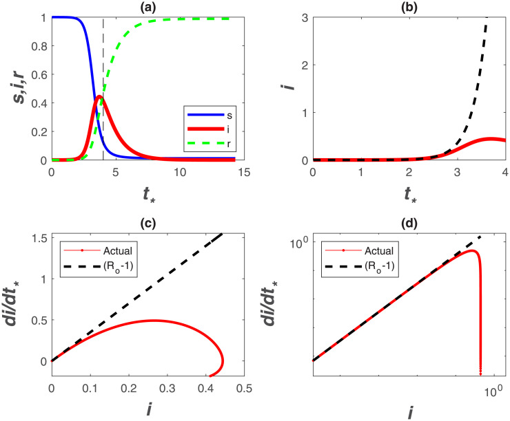
An illustration of the normalized SIR dynamics during an epidemic is shown in Fig 2a, where s, i, and r are numerically solved when setting Ro = 4.5, γ = (1/14) d−1 and So = 100, 000. For small t*(< 1), s ≈ 1 as seen from Fig 2a. In this early phase, s(≈ 1) can be ‘de-coupled’ from i resulting in an autonomous budget for i given as
| (8) |
When Ro > 1, di/dt* > 0 leading to an epidemic or, conversely, a containment of the disease. The solution of Eq (8) is an exponential function i(t)/i(0) = exp[(Ro − 1)t*] shown in Fig 2b.
Fig 2. Phase space and temporal trends of the SIR model.
(a) S(t), I(t), R(t) normalized by So as a function of dimensionless time t* = γt with So = 100, 000, γ = (1/14) d−1, and Ro = 4.5. (b) i = I/So in dimensionless time t* = γt for early times t* < 1 revealing strictly exponential growth (dashed) and deviations from exponential (SIR solution). (c) di/dt* with i in linear and (d) double-log representations. The dashed line is (Ro − 1) where Ro = 4.5. Declines from the dashed line reflect the incipient point where i(t) deviates appreciably from exponential growth. Note how the early-time slope (Ro − 1) is emphasized in the double-log representation.
The Ro may be determined by regressing log(i) against t, and the slope of this regression determines Ro when γ can be separately estimated. More sophisticated fitting procedures can also be conducted on sampled I(t) versus t. A major limitation to this exercise is that I(t) at early times, often determined from reported confirmed cases, is uncertain and depends on testing frequency that may vary in time as I increases. An alternative is to regress di/dt* upon i at early times to detect the highest slope, which can then be used to infer Ro. This approach is featured in Fig 2c, which illustrates that the SIR dynamics exhibit rapid deviations from a linear di/dt* with i set by early times thereby underestimating Ro (for a given γ). Evidently, inference of Ro requires estimates of early time slope, which cannot be easily detected in practice.
A non-conventional approach is to present confirmed infection data using a double-log representation of di/dt* versus i, which is featured in Fig 2d. This presentation has a number of advantages and limitations in the analysis of COVID-19 discussed elsewhere [29]. The main advantage is that the early time slope (= Ro − 1) visually persists over much of the graph. A significant decline in di/dt* is also required before ‘registering’ a drop in such a representation. This insensitivity to moderate declines in di/dt* from its initial value may be advantageous in Ro estimates. The other main limitation, which is inherent to all such analyses, is shifts in testing frequency at high i, and thus the increase in confirmed cases due to expanded testing. It is to be noted that a log-log representation will be more robust to these shifts, because the overall graph will be biased by the initial slope prior to the initialization of expanded testing. Such bias should lead to increases in di/dt* versus i, not declines from the initial slope (Ro − 1) that can be detected. As later shown, such an increase has been noted in several data sets.
With this representation, it is now shown that initial inaction to COVID-19 across many countries around the globe allowed an ensemble estimate of the uncontrolled Ro. Because Ro is likely to be at maximum when no action to COVID-19 are implemented early on, a maximum theoretical ‘boundary-line’ can then be derived to describe the spread of COVID-19 for large So (on log-log representation). This boundary-line analysis can then be used as a logical reference to assess whether measures to reduce β are effective.
Results and discussion
Estimating an early-time Ro
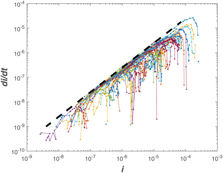
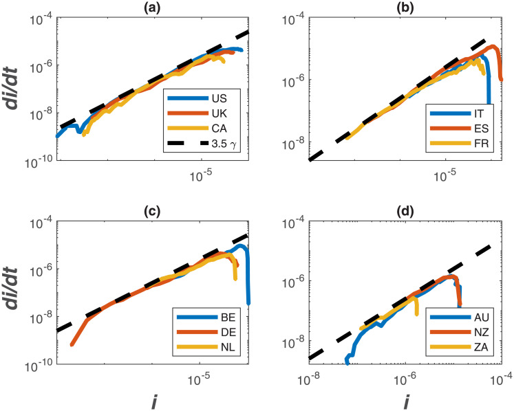
The same log-log scheme featured in Fig 2d is now applied to the global data set supplied by the European Center for Disease Prevention and Control (ECDPC). The data source provides daily confirmed infections I(t) and deaths reported for each country. The population of each country, used to estimate So (i.e. all members are susceptible), was obtained from the 2018 United Nations census and provided as part of the ECDPC data base. While daily data are supplied, not all countries report consistently on a daily I(t). For this reason, daily data on infections were smoothed with a 7 day block-average and dI/dt was estimated from the smoothed data. The 7-day block smooths out some of the spurious reporting during certain time periods (e.g. over weekends or during days when the health-care system was overwhelmed and processing along with reporting delayed by few days). It is to be noted here that the abscissa and ordinate are normalized by the same country-level population, meaning that the actual magnitude of So is not essential. However, such normalization allows for country-to-country comparisons in the same phase-space. The results show a global convergence to Ro = 4.5 from early time-analysis in Fig 3. Examples for specific countries are also featured in Fig 4 illustrating the same early slope patterns. Mindful of all the pitfalls in determining Ro [17], the global estimate here of Ro = 4.5 is roughly commensurate with other entirely independent estimates for COVID-19 discussed in the appendix and featured in Fig 1. The most recent update from a China study suggests an Ro = 4.1 [30] whereas for France, the most recent estimate for early times is Ro = 4.9 [31]. The initially reported and the much cited Ro = 2.2 value [4] from Wuhan, China appears to be low [32] as already noted in Fig 1. A more elaborate estimate of Ro based on case reports, incubation periods, high-resolution real-time human travel data, infection data combined with agent-based mathematical models result in Ro = 4.7 − 6.6 [32]. Other studies report values between 3.3 and 6.6 [33]. It must be emphasized that the Ro determined here reflects ‘country-scale’ early times assuming the entire country population to be So, γ = (1/14)d−1 and does not accommodate any early measures enacted to reduce β or increase γ, which were undertaken in China [13] and other countries (e.g. Germany).
Fig 3. Comparison between di/dt and i for 57 countries.
The dashed line is (Ro − 1)γ, where Ro = 4.5, and γ = (1/14)d−1. Negative deviations from the dashed line reflect deviations from exponential in this phase-space representation.
Fig 4. Same as Fig 3 but for sample countries.
(a) the United States of America (US), the United Kingdom (UK), and Canada (CA); (b) Italy (IT), Spain (ES), and France (FR); (c) Belgium (BE), Germany (DE), the Netherlands (NL); (d) Australia (AU), New Zealand (NZ), and South Africa (ZA).
Sub-national dynamics and interventions
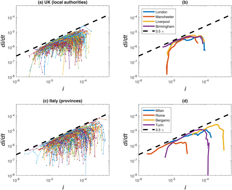
The same analysis performed for World countries is now applied at a sub-national level, considering Upper Tier Local Authorities (UTLAs) in the UK and provinces in Italy (Fig 5). Results show a higher variability than country-level data (as expected) but the theoretical ‘boundary-line’ of Ro = 4.5 is shown to hold also at finer spatial scales. Cases reported at the beginning of April demonstrate that UK regions are at an early phase of the epidemics (with more ramp-up in testing as later discussed), while Italian provinces are approaching the peak of infections due to strict interventions put in place by national authorities.
Fig 5. Same as Fig 3 but for sample UTLAs in the UK (a) and provinces in Italy (c).
Selected UTLAs and provinces are shown in panels b and d, respectively.
Non-pharmaceutical interventions (e.g., social distancing, hand washing, universal masking) are the only measures currently available to limit the spread of COVID-19 [34], while contact tracing and isolation have been implemented to contain infected individuals [35]. Simulation results [35] showed that a COVID-19 outbreak can be controlled within 3 months if such strategies are put in place rapidly and effectively. This has been confirmed in another study [36] that showed that the containment measures employed in China and aimed at reducing human-to-human aerial transmission, succeeded in reducing the reproduction number to below unity within 30 days from implementation.
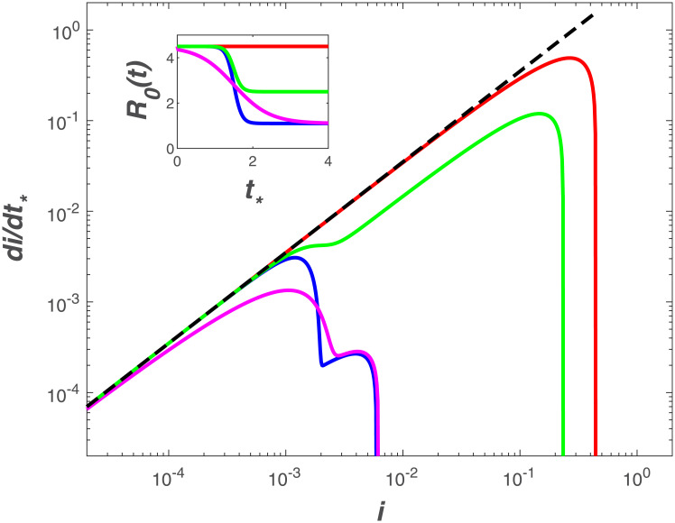
To consider the impact of interventions that reduce the infection rate over time and have direct effects on local scale dynamics [13], a time-varying Ro, labelled as Ro,d (i.e. dynamic) can be implemented in the SIR model. A logistic function captures temporal patterns in Ro,d, the effective reproduction number, consistent with those estimated for other outbreaks [36–39],
| (9) |
where Rc is the controlled value of the dynamic Ro,d, kc is the steepness of the intervention curve, and t50 is the time when Ro,d = (Rc + Ro)/2. It is assumed that, through interventions, the initial Ro = 4.5 is reduced to a controlled value of Rc = 1.1 after 2/γ days.
Model results accounting for different intervention scenarios (Fig 6) resemble the trends observed in the Italian provinces with the timing and magnitude of Ro reductions shifting the linear relation down and decreasing the maximum fraction of infected individuals. Such jumps are smoothed over at the national level where a clear deviation from exponential is observed (Fig 4).
Fig 6. Modeled di/dt* as a function of i when considering a dynamic Ro,d.
Five scenarios are illustrated (inset): no intervention (red) with Ro = 4.5 set to its uncontrolled value, Ro,c = 1.1 (epidemic near containment) and kc = 0.7 (blue), Ro,c = 1.1 and kc = 0.15 (magenta), Ro,c = 2.5 (typical of countries with strong initial intervention) and kc = 0.7 (green). The other parameters of the logistic functions are Ro,u = 4.5 and t50 = 1.5/γ.
An alternative hypothesis: Power-law vs exponential
Whether these results are suggestive of a global convergence to an uncontrolled Ro = 4.5 or to some other dimensionless property must not be overlooked. A linear relation on a log-log representation may also be indicative of power-law solutions at early times, already documented in a number of studies for COVID-19 [40, 41]. In fact, published analysis of infection data from the top 25 affected countries reveals approximate power-law behavior of the form I(t) ∼ ta (or log(i) = a log(t) + b) with two different growth patterns [40]: steady power law growth with moderate scaling exponents (i.e., a = 3-5) or explosive power law growth with dramatic scaling exponents (i.e., a = 8-11).
Within the confines of the SIR dynamical system framework here, we ask: what are the necessary modifications to obtain power-law solutions at early times? Such a solution, while not unique, may be possible by revising the force of infection as βim. The original SIR model is recovered when m = 1. For this non-linear force of infection, the SIR system becomes
| (10) |
| (11) |
| (12) |
This revision ensures that the total population maintains its constant value (≈ So here). The early times dynamics (i.e. S(t) ≈ So) for the non-dimensional infection compartment i are now governed by
| (13) |
When m < 1, maintaining a definition of Ro > 1 (epidemic), and noting that i ≪ 1, the first term on the right-hand side of Eq (13) is much larger than the second term. In fact, to obtain a maximum exponent enveloping the early-time relation between di/dt* and i, the linear term can be dropped so that di/dt* ≈ Ro im (only a growth phase). On a log-log representation, log(di/dt*) = m log(i) + log(Ro). A constant slope such as those featured in Figs 3 and 4 may simply be estimates of m (instead of Ro). The initial conjecture is that a power-law solution emerges from the modified SIR dynamics when m < 1. However, the slope here (= 3.5) actually exceeds unity contradicting this revised analysis. This finding supports the view that a global convergence to an uncontrolled Ro = 4.5 is a more likely explanation than a power-law alternative arising from a non-linear force of infection. To be clear, there are other causes for power-law solutions (e.g. a stochastic β as discussed elsewhere [42]), but those fall outside the domain of deterministic SIR approaches adopted here. Nonetheless, and as a bridge between the studies reporting power-law growth in time for i and the modified SIR here, a relation between m and a is sought. The solution to Eq (13) can be expressed as
| (14) |
which is a power-law in t. For dimensionless time γt >> i(0)1−m/[Ro(1 − m)], i(t) ∼ t1/(1−m) (m < 1). It directly follows that m = (a − 1)/a < 1 (as expected), where a > 1 is determined by regressing early-times log(i) versus log(t). Reported a for what has been termed as ‘explosive’ cases such as the US, UK Canada, Russia, among others [40] all yield an a > 8 (with the US a > 16). Such high a simply confirms that m ≈ 1 (and without much variations), and the early time SIR dynamics does describe reasonably those cases. For low a values, termed as ‘steady’, the mean a ≈ 4.8, and thus yields an m ≈ 0.8, still not too far from unity. The shortcoming of analyzing I(t) upon t is that absolute figures of I(t) are sensitive to increased COVID-19 testing in time, which is considered next.
Impact of testing ramp-up
A further explanation of early-time deviation from the SIR model (noted in several data sets here) may be time-dependent ramp-up of testing, which reveals existing infections at a rate faster than the infection spread. This hypothesis can be implemented in the SIR model considering the temporal dynamics of the testing capacity, f. Data show that testing capacity rates of increase depend on the country and follow linear or saturating trends [43]. To model a testing capacity that starts small and saturates over time, we assumed the maximum fraction of individuals that can be tested is f = 1, tests are 100% true and evenly distributed across compartments, and testing capacity grows exponentially at a rate k, independent of I, giving, f(t) = 1 − exp(−kt). Therefore, the apparent number of infections, ia, initially grows according to the superposition of the infectious spread rate and testing capacity increase rate, i.e., exp[(R0 − 1 − k)t] and log(dia/dt) ∼ (R0 − 1 − k)log(ia). From the data [43], we estimate a typical value of k is 0.02 d−1, which is negligible when compared to Ro − 1. The small value of k relative to Ro − 1 indicates that the imprint of testing ramp-up likely does not strongly impact the observed early-time dynamics and the observed convergent slope remains a robust indicator of the early phases of virus dynamics.
The role of super-spreaders on Ro estimates
For COVID-19, there is currently no general agreement on a precise definition of a super-spreader. In its broadest interpretation, a super-spreader has the propensity to infect a larger than average number of susceptible individuals. This definition does not have a unique link to a precise mechanism and appears to encompass biological, behavioral and environmental variables relevant to disease transmission. We consider a narrow view of super-spreaders as those infectious individuals with high mobility. Within this narrower scope, the concern is to assess how long-distance mobility of few infected individuals (i.e. super-spreaders) impacts the estimates of Ro when the phase-space analysis of early times dynamics is used. Because these infectious individuals are highly mobile and depending on the mobility network in each country or region, detailed country-by-country investigation is beyond the scope here. However, the mobility of these super-spreaders can impact the much discussed mass-action assumption in SIR and thus estimates of Ro from early times dynamics.
We address this effect using an idealized yet generic analysis similar to the ramp-up testing effect earlier discussed. To do so, a country is first divided into identical and equal sized regions each of area given by dx and dy. These regions are ‘isolated’ and experience their own identical SIR dynamics assuming the same Ro and γ. Few infectious individuals arrive into this country (treated as a lattice in an x − y plane) at random locations thereby initially infecting few regions. Area wise, under 0.01% of the country area experiences an infectious individual at t = 0. To amplify the role of super-spreaders, mobility is only allowed between regions by super-spreaders, whereas mass action is still assumed between I and S within each region. To allow for large mobility of these super-spreaders in the SIR analysis, the budget equation for I in each region is revised to become an integro-differential equation (IDE) given as [44]
| (15) |
where all state variables now evolve in space (x, y) and time (t) so that I, S, and R represent I(x, y, t), S(x, y, t), and R(x, y, t) (unless otherwise stated), No is the initial population in dx by dy region (So is the entire country population), ϕ(<< 1) is the fraction of infectious individuals that are mobile in a region within a given time step dt (super-spreaders of the I budget) and p(x′, y′) describes their spread kernel defined by the probability that infectious individuals at position x, y move to position x′, y′ in a time increment dt. The spread kernel must satisfy the normalizing condition
| (16) |
When ϕ = 0 (no super-spreaders), the IDE approach reduces to spatially independent or autonomous SIR models operating in compartments dx × dy with no connectivity or spatial interaction between compartments (i.e. the entire country comprised of regions will experience the same Ro).
A number of choices can be made about p(x′, y′), which all depend on the mobility network in each country (airports, roads, trains, public-transport, etc.) and analyzing all of them is beyond the scope here. For simplicity, we selected a distance-dependent spatial spread kernel [45]
| (17) |
where r2 = (x − xo)2 + (y − yo)2, σ is a measure of the spread of the spatial kernel, and αN is a normalizing constant. Since the interest here is in spatial spread kernels with finite support Ra (i.e. super-spreaders cannot travel to all the corners of the domain in a single dt), αN is determined so that
| (18) |
This condition yields [45]
| (19) |
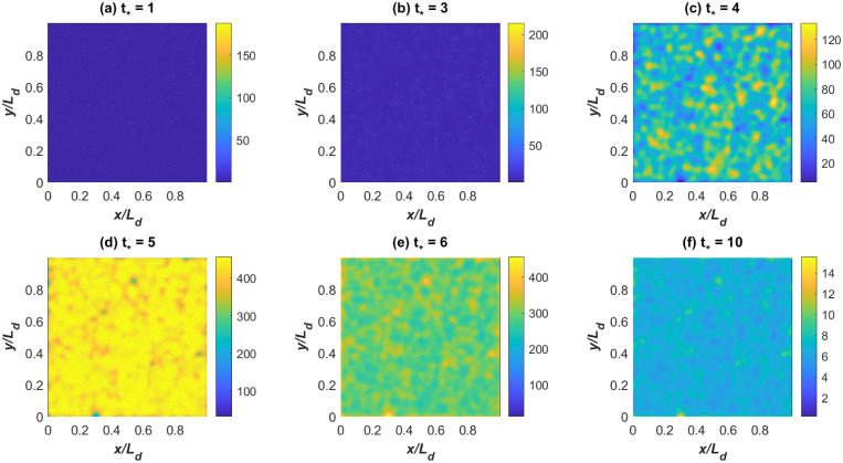
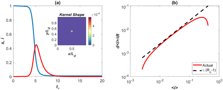
Other spatial kernels can be specified and subjected to the same normalizing conditions thereby making the IDE approach flexible in terms of choices about spatial spread of infectious individuals. Also, it is possible to include time dependency in the spreading properties, meaning p(x′, y′, t) changes in time through temporal variations in Ra or σ or both (e.g. to allow for diurnal variations in mobility habits). Model calculations using the Gaussian kernel in Fig 7 show that super-spreaders (ϕ = 0.001) will infect almost the entire domain by t* = 5. The main difference between Fig 2 and the spatially aggregated SIR model in Fig 8 is an initial delay and the occurrence of a rapid rise resembling the data from the UK and Italy regions at early times. However, beyond this initial delay in spreading, the early times dynamics with super-spreaders and without them are commensurate. That is, the effects of super-spreaders resembles the impact of testing ramp-up earlier discussed on the phase-space of di/dt* versus i but with delays.
Fig 7. SIR model with super-spreaders.
Modeled I(x, y, t) at selected t* = γt showing the progression of disease outbreak in space due to mobility of super-spreaders only.
Fig 8. SIR model with super-spreaders: spatially integrated results.
(a) Modeled < s(t) > and < i(t) >, where < . > is spatially integrated quantities (the inset shows the Gaussian spatial spread kernel). (b) The early times dynamics showing the effects of super-spreaders in the phase of d < i >/dt versus < i >. The line (Ro − 1)γ with Ro = 4.5 is shown for reference. This effect is similar to those reported in the UK and Italy regions.
Size of the epidemic
The maximum infections Imax (where dI/dt = 0) can be derived as a function of So and Ro by first dividing the budgets of dS/dt and dI/dt, solving the resulting equation, and noting that dI/dt = 0 when S(t)/So = γ/β = 1/Ro at Imax to yield
| (20) |
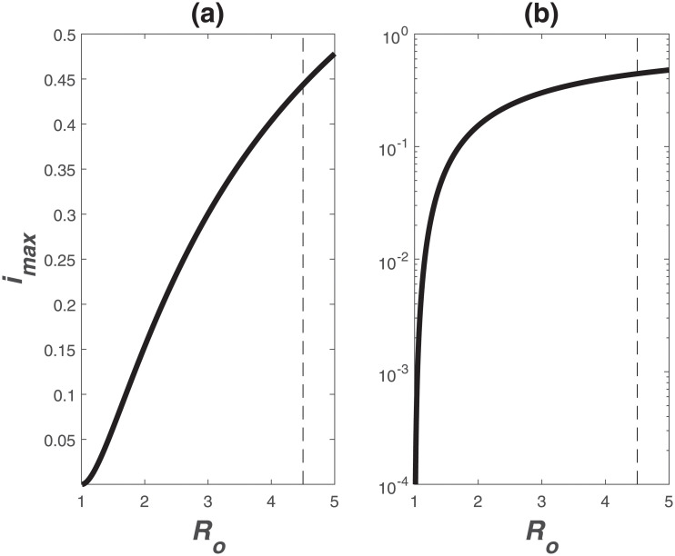
Variations of imax versus Ro are featured in Fig 9.
Fig 9. Relation between maximum infection fraction imax = Imax/So and Ro.
For Ro = 4.5, imax = 0.44, which is much higher than values obtained for the common cold or the flu (Ro = 2 − 3) or influenza (Ro = 1.4 − 2.8).
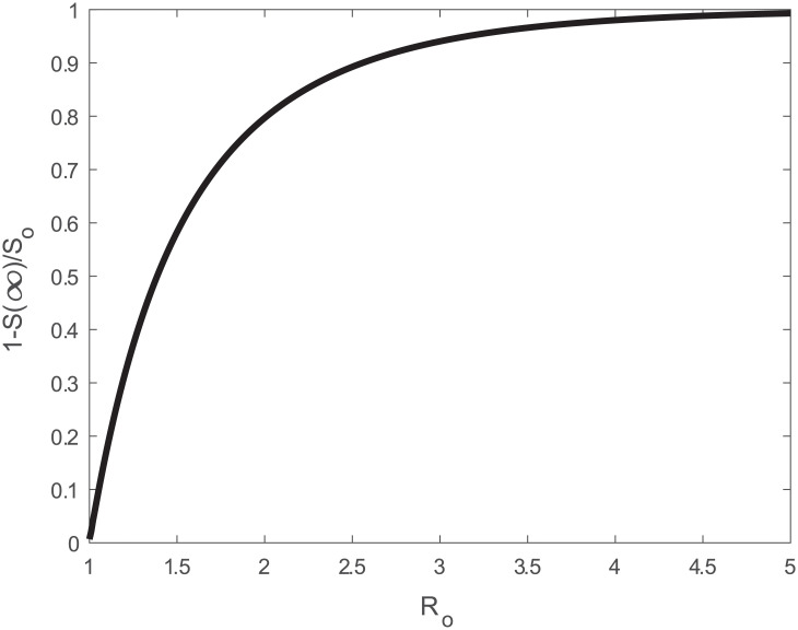
The most significant use of Ro is an estimate of the size of the epidemic. The total fraction of infected individuals may be inferred from 1 − S(∞)/S(0), where S(∞)/S(0) = 1 − R(∞)/S(0) > 0 because I(∞) = 0. The relation between S(t) and R(t) can be derived
| (21) |
which when integrated between t = 0 and t = ∞ yields,
| (22) |
The solution for S(∞)/So can be analytically derived and linked to the total infected individuals IT using
| (23) |
where W[z] is the Lambert W-function of argument z. For pre-specified Ro, the behavior of the IT/So individuals is shown in Fig 10. With such a high Ro = 4.5, some 98% of the population will be infected as t* → ∞. When mortality is assumed to be some fraction of IT, then the mortality fraction is Mo/So = αm[1−S(∞)/S(0)].
Fig 10. Relation between total infection fraction 1 − S(∞)/So and Ro.
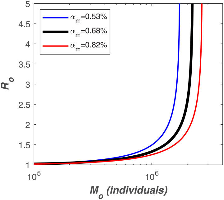
Different definitions of the global mortality rate αm have been considered but, for the purposes of the present study, the ratio of deaths to both symptomatic and asymptomatic cases is most appropriate. This ratio is dubbed the Infection Fatality Rate (IFR) and is different from the Case Fatality Rate (CFR), which is the ratio of deaths to the number of confirmed cases. The IFR is more appropriate because the ‘Infected’ compartment of the SIR model comprises of both symptomatic and asymptomatic individuals. According to the latest IFR estimates, αm ranges between 0.53 and 0.82% with a mean value of 0.68% [46].
For the USA, the epicenter of COVID-19 at the time of submission of this article on April 10, 2020, we asked how much Ro should be reduced by deliberate intervention to maintain mortality below a certain threshold size Mo. With S(0) = 327M, we determine how much Ro should be reduced as a function of Mo assuming different values of αm. These results are featured in Fig 11 and suggest that to maintain mortality below 1 million, Ro < 1.5 when αm = 0.53%, a reduction factor of 3 over its uncontrolled value. Under the same scenario, to limit the death toll below 300 thousand people, Ro should be reduced to 1.1, a reduction factor of 4. These reduction factors are not entirely unreasonable using non-pharmaceutical measures (social distancing, masks, hand sanitizing, etc…).
Fig 11. Relation between total mortality (Mo) and Ro for different values of αm and assuming So = 327M.
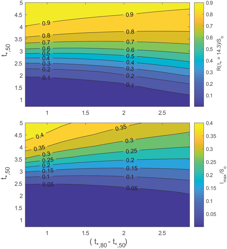
A natural extension of this exercise is to consider temporal changes in Ro following the logistic form in Eq (9). The maximum number of infected Imax at time t and cumulative number of infections R(∞) ≈ R(t* ≈ 14) can be made to vary as the slope kc and t50 are changed (Eq (9)). A larger kc signifies more rapid enforcement of intervention policies and a larger t50 represents later enforcement. To provide a physical meaning for kc, we define as the time after first infection at which Ro is fo% of the way through its total decline from Ro,u to Ro,c. With these definitions, . An obvious choice for Ro,u = 4.5, the global average when no intervention is enforced. A logical choice for fo = 80% and is consistent with the point at which the logistic function enters the ‘flattening phase’. We choose Ro,c = 1.0 to represent the most optimistic scenario of a near-containment by non-pharmaceutical intervention. For reference, the South Korea data suggests that early intervention, even when rapidly enforced shortly after the outbreak, resulted in Ro = 1.5 [47]. The effectiveness of interventions and any delays can now be linked to mortality and severity by varying t50 and t80. Fig 12 presents how R(t* ≈ 14) and Imax are contained for only a restricted envelope of speed and timeliness of policy enforcement. The R(t* ≈ 14) represents the cumulative number of fatalities and Imax is proportional to the degree to which resources, like hospital intensive care units, will be overwhelmed at peak infection rate. The results in Fig 12 indicate that if Ro > 2.7 within t = 3.5/γ (about 49 d here), a more than 10% reduction relative to So in Imax or R(∞) is unlikely.
Fig 12. Variation in cumulative number of infected relative to So (top) and in maximum number of infected relative to So (bottom).
The logistic form of Ro was used (Eq (9)). The Ro was set to vary from Ro,c = 4.5 to Ro,u = 1.0. The t*,50 and t*,80 are the dimensionless times at which Ro is half and 80% through the the total decline.
An implication of Fig 12 is that if Ro does not decrease to at least 2.7 by 44 days after first infection, more than a million people are expected to die with an assumed constant mortality rate of 0.53%. For mortality to be confined to a range in the 100,000, then a reduction of Ro from 4.5 to 2.7 must be achieved within 14 days of first infection, which did not occur in the USA. As of July 30, 2020, confirmed fatalities in the USA have exceeded 150,000.
Last, it is to be noted that the fraction of individuals that must be immune (either through vaccination or recovery from prior COVID-19 infections) must exceed the herd immune threshold (HIT), which is given by
| (24) |
This estimate of HIT sets the limit on the immune population needed to overcome another COVID-19 pandemic (assuming a global constant Ro = 4.5 and no intervention). Should immunity from prior COVID-19 infections be transient, this estimate then sets the upper bound on the fraction of population that must be vaccinated and the vaccine needed in the future.
Conclusion
The work here has shown a global convergence of Ro = 4.5 when no deliberate intervention was taken for COVID-19. This Ro was shown to describe reasonably the maximum initial exponential growth rate of COVID-19 (=(Ro − 1)γ, where γ = (1/14)d−1) in many countries that did not initiate preventive measures within γt = 2. The findings here further support the growing consensus that the initial Ro = 2.2 estimate from Wuhan, China is low. The value of Ro = 4.5 is much more in line with other estimates (Ro = 4 − 6) derived from far more complex models. Model calculations and theoretical considerations offered here delineate the conditions when this Ro estimate is robust to the inclusion of other mechanisms such as super-spreaders and ramp-up in initial testing. The critical herd immunity level that must be reached is 78% to ensure COVID-19 does not become an epidemic again. This estimate sets a maximum limit on the vaccination required.
Appendix: Compilation of Ro estimates from previous studies
A recent review [21] showed that existing estimates of Ro range from 1.4 to 6.49, with a mean of 3.28 and an interquartile range of 1.16. Early studies reported lower Ro values [21] and results often vary with the estimation method. Stochastic, statistical, and mathematical methods provided mean estimates of 2.44, 2.67, and 4.2, respectively [21], and SIR-based approaches are likely to provide higher values compared to other methods [36]. Similar results were presented in another meta-analysis [48] reporting a mean R0 of 3.38 (values ranging between 1.90 to 6.49) but did not find a significant effect of different estimation methods. A summary of these results is provided in Table 1.
Table 1. Compilation of published Ro estimates.
| Reference | R0 | R0 range | Study date |
|---|---|---|---|
| (e.g. 95% CI) | (from-to) | ||
| Sanche et al. [22] | 5.7 | 3.8—8.9 | 15 Jan. 2020—30 Jan. 2020 |
| Li et al. [4] | 2.2 | 1.4—3.9 | N/A—22 Jan. 2020 |
| Wu et al. [49] | 2.68 | 2.47- 2.86 | 31 Dec. 2019—28 Jan. 2020 |
| Riou and Althaus [50] | 2.2 | 1.4—3.8 | N/A—18 Jan. 2020 |
| Liu et al. [39] | 4.5 | 4.4—4.6 | N/A—07 Feb. 2020 |
| Zhang et al. [51] | 5.6 | 5.3—5.8 | 21 Jan. 2020—20 Feb. 2020 |
| Shen et al. [52] | 4.7 | 4.50—4.92 | 12 Dec. 2019—22 Jan. 2020 |
| Liu et al. [53] | 2.90 | 2.32—3.63 | N/A—23 Jan. 2020 |
| Liu et al. [53] | 2.92 | 2.28—3.67 | N/A—23 Jan. 2020 |
| Read et al. [54] | 3.11 | 2.39—4.13 | 01 Jan. 2020—22 Jan. 2020 |
| Majumder and Mandl [55] | 2.55 | 2.0—3.1 | 08 Dec. 2019—26 Jan. 2020 |
| WHO (from [21]) | 1.95 | 1.4—2.5 | N/A—18 Jan. 2020 |
| Cao et al. [30] | 4.08 | 3.37—4.77 | N/A—23 Jan. 2020 |
| Zhao et al. [56] | 2.24 | 1.96—2.55 | 10 Jan. 2020—24 Jan. 2020 |
| Zhao et al. [56] | 3.58 | 2.89—4.39 | 10 Jan. 2020—24 Jan. 2020 |
| Imai et al. [57] | 2.6 | 1.5—3.5 | N/A—18 Jan. 2020 |
| Tang et al. [58] | 6.47 | 5.71—7.23 | N/A—22 Jan. 2020 |
Data Availability
Daily confirmed COVID-19 infections in World countries are available at \url{https://www.ecdc.europa.eu/en/publications-data/download-todays-data-geographic-distribution-covid-19-cases-worldwide} (accessed on 08/04/2020). The dataset includes population estimates for each country as obtained from the 2018 United Nations census. Reported cases for UTLAs in the UK and provinces in Italy were obtained from \url{https://www.gov.uk/government/publications/covid-19-track-coronavirus-cases} (accessed on 09/04/2020) and \url{https://github.com/pcm-dpc/COVID-19} (accessed on 09/04/2020), respectively. Population counts for UTLAs and Italian provinces are available at \url{https://www.ons.gov.uk/peoplepopulationandcommunity/populationandmigration/populationestimates/datasets/populationestimatesforukenglandandwalesscotlandandnorthernireland} (accessed on 04/04/2020) and \url{http://dati.istat.it/Index.aspx?DataSetCode=DCIS_POPRES1} (accessed on 03/04/2020), respectively.
Funding Statement
The authors received no specific funding for this work.
References
- 1. Dietz K, Heesterbeek J. Daniel Bernoulli’s epidemiological model revisited. Mathematical Biosciences. 2002;180(1-2):1–21. 10.1016/S0025-5564(02)00122-0 [DOI] [PubMed] [Google Scholar]
- 2. Buckee C, Balsari S, Chan J, Crosas M, Dominici F, Gasser U, et al. Aggregated mobility data could help fight COVID-19. Science. 2020; 10.1126/science.abb8021 [DOI] [PubMed] [Google Scholar]
- 3. Ross R. An application of the theory of probabilities to the study of a priori pathometry: Part I. Proceedings of the Royal Society of London Series A—Containing papers of a mathematical and physical character. 1916;92(638):204–230. [Google Scholar]
- 4. Li Q, Guan X, Wu P, Wang X, Zhou L, Tong Y, et al. Early transmission dynamics in Wuhan, China, of novel coronavirus–infected pneumonia. New England Journal of Medicine. 2020;382:1199–1207. 10.1056/NEJMoa2001316 [DOI] [PMC free article] [PubMed] [Google Scholar]
- 5. Layne S, Hyman J, Morens D, Taubenberger J. New coronavirus outbreak: Framing questions for pandemic prevention. Science Translational Medicine. 2020;12 10.1126/scitranslmed.abb1469 [DOI] [PMC free article] [PubMed] [Google Scholar]
- 6. Kermack W, McKendrick A. A contribution to the mathematical theory of epidemics. Proceedings of the Royal Society of London Series A-Containing papers of a mathematical and physical character. 1927;115(772):700–721. [Google Scholar]
- 7. Anderson R, May R. Population biology of infectious diseases: Part I. Nature. 1979;280(5721):361–367. 10.1038/280361a0 [DOI] [PubMed] [Google Scholar]
- 8. Hethcote H. The mathematics of infectious diseases. SIAM Review. 2000;42(4):599–653. 10.1137/S0036144500371907 [DOI] [Google Scholar]
- 9. Keeling M, Danon L, et al. Mathematical modelling of infectious diseases. British Medical Bulletin. 2009;92(1):33–42. 10.1093/bmb/ldp038 [DOI] [PubMed] [Google Scholar]
- 10. Keeling M, Rohani P. Modeling Infectious Diseases in Humans and Animals. Princeton University Press; 2011. [Google Scholar]
- 11. Blackwood J, Childs L. An introduction to compartmental modeling for the budding infectious disease modeler. Letters in Biomathematics. 2018;5(1):195–221. 10.30707/LiB5.1Blackwood [DOI] [Google Scholar]
- 12. Walters C, Meslé M, Hall I. Modelling the global spread of diseases: A review of current practice and capability. Epidemics. 2018;25:1–8. 10.1016/j.epidem.2018.05.007 [DOI] [PMC free article] [PubMed] [Google Scholar]
- 13. Maier B, Brockmann D. Effective containment explains subexponential growth in recent confirmed COVID-19 cases in China. Science. 2020; 10.1126/science.abb4557 [DOI] [PMC free article] [PubMed] [Google Scholar]
- 14. Heffernan J, Smith R, Wahl L. Perspectives on the basic reproductive ratio. Journal of the Royal Society Interface. 2005;2(4):281–293. 10.1098/rsif.2005.0042 [DOI] [PMC free article] [PubMed] [Google Scholar]
- 15. Ridenhour B, Kowalik J, Shay D. Unraveling R0: Considerations for public health applications. American Journal of Public Health. 2018;108(S6):S445–S454. 10.2105/AJPH.2013.301704r [DOI] [PMC free article] [PubMed] [Google Scholar]
- 16. Keeling M, Grenfell B. Individual-based perspectives on R0. Journal of Theoretical Biology. 2000;203(1):51–61. 10.1006/jtbi.1999.1064 [DOI] [PubMed] [Google Scholar]
- 17. Delamater P, Street E, Leslie T, Yang Y, Jacobsen K. Complexity of the basic reproduction number(R0). Emerging Infectious Diseases. 2019;25(1):1–4. 10.3201/eid2501.171901 [DOI] [PMC free article] [PubMed] [Google Scholar]
- 18. Pybus OG, Charleston MA, Gupta S, Rambaut A, Holmes EC, Harvey PH. The epidemic behavior of the hepatitis C virus. Science. 2001;292(5525):2323–2325. 10.1126/science.1058321 [DOI] [PubMed] [Google Scholar]
- 19. Lipsitch M, Cohen T, Cooper B, Robins JM, Ma S, James L, et al. Transmission dynamics and control of severe acute respiratory syndrome. Science. 2003;300(5627):1966–1970. 10.1126/science.1086616 [DOI] [PMC free article] [PubMed] [Google Scholar]
- 20. Mills CE, Robins JM, Lipsitch M. Transmissibility of 1918 pandemic influenza. Nature. 2004;432(7019):904–906. 10.1038/nature03063 [DOI] [PMC free article] [PubMed] [Google Scholar]
- 21. Liu Y, Gayle AA, Wilder-Smith A, Rocklöv J. The reproductive number of COVID-19 is higher compared to SARS coronavirus. Journal of Travel Medicine. 2020;27:1–4. 10.1093/jtm/taaa021 [DOI] [PMC free article] [PubMed] [Google Scholar]
- 22. Sanche S, Lin YT, Xu C, Romero-Severson E, Hengartner N, Ke R. Early Release-High Contagiousness and Rapid Spread of Severe Acute Respiratory Syndrome Coronavirus 2. Emerging Infectious Diseases. 2020;26(7):1470–1477. [DOI] [PMC free article] [PubMed] [Google Scholar]
- 23. Lauer SA, Grantz KH, Bi Q, Jones FK, Zheng Q, Meredith HR, et al. The incubation period of coronavirus disease 2019 (COVID-19) from publicly reported confirmed cases: estimation and application. Annals of Internal Medicine. 2020;172(9):577–582. 10.7326/M20-0504 [DOI] [PMC free article] [PubMed] [Google Scholar]
- 24. Murray J. Mathematical Biology: I. An Introduction. vol. 17 Springer Science & Business Media; 2007. [Google Scholar]
- 25.Organization WH. Report of the WHO-China Joint Mission on Coronavirus Disease 2019 (COVID-19). World Health Organization; 2020. Available from: https://www.who.int/docs/default-source/coronaviruse/who-china-joint-mission-on-covid-19-final-report.pdf.
- 26. Verity R, Okell L, Dorigatti I, Winskill P, Whittaker C, Imai N, et al. Estimates of the severity of coronavirus disease 2019: a model-based analysis. The Lancet Infectious Diseases. 2020; 10.1016/S1473-3099(20)30243-7 [DOI] [PMC free article] [PubMed] [Google Scholar]
- 27. Newman M. Networks. Oxford university press; 2018. [Google Scholar]
- 28. Barbour A, Mollison D. Epidemics and Random Graphs In: Stochastic Processes in Epidemic Theory. Springer; 1990. p. 86–89. [Google Scholar]
- 29.minutephysics. How To Tell If We’re Beating COVID-19. YouTube; 2020. Available from: https://www.youtube.com/watch?v=54XLXg4fYsc&list=PLFEVngVI8GheUoZw2B869Yw-R6xjQc9ev&index=35&t=281s.
- 30. Cao Z, Zhang Q, Lu X, Pfeiffer D, Jia Z, Song H, et al. Estimating the effective reproduction number of the 2019-nCoV in China. medRxiv. 2020;. [Google Scholar]
- 31.Roques L, Klein E, Papaix J, Soubeyrand S. Mechanistic-statistical SIR modelling for early estimation of the actual number of cases and mortality rate from COVID-19. arXiv preprint arXiv:200310720. 2020;.
- 32.Sanche S, Lin Y, Xu C, Romero-Severson E, Hengartner N, Ke R. The novel coronavirus, 2019-nCoV, is highly contagious and more infectious than initially estimated. arXiv preprint arXiv:200203268. 2020;.
- 33. Yuan J, Li M, Lv G, Lu Z. Monitoring Transmissibility and Mortality of COVID-19 in Europe. International Journal of Infectious Diseases. 2020; 10.1016/j.ijid.2020.03.050 [DOI] [PMC free article] [PubMed] [Google Scholar]
- 34. Haushofer J, Metcalf CJE. Which interventions work best in a pandemic? Science. 2020;368(6495):1063–1065. 10.1126/science.abb6144 [DOI] [PubMed] [Google Scholar]
- 35. Hellewell J, Abbott S, Gimma A, Bosse NI, Jarvis CI, Russell TW, et al. Feasibility of controlling COVID-19 outbreaks by isolation of cases and contacts. The Lancet Global Health. 2020;8:e488–e496. 10.1016/S2214-109X(20)30074-7 [DOI] [PMC free article] [PubMed] [Google Scholar]
- 36. You C, Deng Y, Hu W, Sun J, Lin Q, Zhou F, et al. Estimation of the time-varying reproduction number of COVID-19 outbreak in China. International Journal of Hygiene and Environmental Health. 2020;228:113555 10.1016/j.ijheh.2020.113555 [DOI] [PMC free article] [PubMed] [Google Scholar]
- 37. Ng TC, Wen TH. Spatially adjusted time-varying reproductive numbers: understanding the geographical expansion of urban dengue outbreaks. Scientific Reports. 2019;9(1):1–12. 10.1038/s41598-019-55574-0 [DOI] [PMC free article] [PubMed] [Google Scholar]
- 38. Liu QH, Ajelli M, Aleta A, Merler S, Moreno Y, Vespignani A. Measurability of the epidemic reproduction number in data-driven contact networks. Proceedings of the National Academy of Sciences. 2018;115(50):12680–12685. 10.1073/pnas.1811115115 [DOI] [PMC free article] [PubMed] [Google Scholar]
- 39. Liu T, Hu J, Xiao J, He G, Kang M, Rong Z, et al. Time-varying transmission dynamics of Novel Coronavirus Pneumonia in China. bioRxiv. 2020; [Google Scholar]
- 40.Singer H. Short-term predictions of country-specific COVID-19 infection rates based on power law scaling exponents. arXiv preprint arXiv:200311997. 2020;.
- 41. Wodarz D, Komarova N. Patterns of the COVID19 epidemic spread around the world: exponential vs power laws. medRxiv. 2020; [DOI] [PMC free article] [PubMed] [Google Scholar]
- 42. Newman M. Power laws, Pareto distributions and Zipf’s law. Contemporary Physics. 2005;46(5):323–351. [Google Scholar]
- 43. Roser M, Ritchie H, E OO, Hasell J. Coronavirus Pandemic (COVID-19). Our World in Data. 2020;. [Google Scholar]
- 44. Pastor-Satorras R, Castellano C, Van Mieghem P, Vespignani A. Epidemic processes in complex networks. Reviews of Modern Physics. 2015;87(3):925 10.1103/RevModPhys.87.925 [DOI] [Google Scholar]
- 45. Fuentes M, Kuperman M, Kenkre V. Nonlocal interaction effects on pattern formation in population dynamics. Physical Review Letters. 2003;91(15):158104 10.1103/PhysRevLett.91.158104 [DOI] [PubMed] [Google Scholar]
- 46. Meyerowitz-Katz G, Merone L. A systematic review and meta-analysis of published research data on COVID-19 infection-fatality rates. medRxiv. 2020;. [DOI] [PMC free article] [PubMed] [Google Scholar]
- 47. Shim E, Tariq A, Choi W, Lee Y, Chowell G. Transmission potential and severity of COVID-19 in South Korea. International Journal of Infectious Diseases. 2020;93:339–344. 10.1016/j.ijid.2020.03.031 [DOI] [PMC free article] [PubMed] [Google Scholar]
- 48. Alimohamadi Y, Taghdir M, Sepandi M. The estimate of the basic reproduction number for novel coronavirus disease (COVID-19): a systematic review and meta-analysis. Journal of Preventive Medicine and Public Health. 2020;. 10.3961/jpmph.20.076 [DOI] [PMC free article] [PubMed] [Google Scholar]
- 49. Wu JT, Leung K, Leung GM. Nowcasting and forecasting the potential domestic and international spread of the 2019-nCoV outbreak originating in Wuhan, China: a modelling study. The Lancet. 2020;395(10225):689–697. 10.1016/S0140-6736(20)30260-9 [DOI] [PMC free article] [PubMed] [Google Scholar]
- 50. Riou J, Althaus CL. Pattern of early human-to-human transmission of Wuhan 2019 novel coronavirus (2019-nCoV), December 2019 to January 2020. Eurosurveillance. 2020;25(4):2000058 10.2807/1560-7917.ES.2020.25.4.2000058 [DOI] [PMC free article] [PubMed] [Google Scholar]
- 51. Zhang KK, Xie L, Lawless L, Zhou H, Gao G, Xue C. Characterizing the transmission and identifying the control strategy for COVID-19 through epidemiological modeling. medRxiv. 2020; [Google Scholar]
- 52. Shen M, Peng Z, Xiao Y, Zhang L. Modelling the epidemic trend of the 2019 novel coronavirus outbreak in China. bioRxiv. 2020; [DOI] [PMC free article] [PubMed] [Google Scholar]
- 53. Liu T, Hu J, Kang M, Lin L, Zhong H, Xiao J, et al. Transmission dynamics of 2019 novel coronavirus (2019-nCoV). bioRxiv. 2020; [Google Scholar]
- 54. Read JM, Bridgen JR, Cummings DA, Ho A, Jewell CP. Novel coronavirus 2019-nCoV: early estimation of epidemiological parameters and epidemic predictions. medRxiv. 2020; [DOI] [PMC free article] [PubMed] [Google Scholar]
- 55. Majumder M, Mandl KD. Early transmissibility assessment of a novel Coronavirus in Wuhan, China. Social Science Research Network (SSRN). 2020; 10.2139/ssrn.3524675 [DOI] [PMC free article] [PubMed] [Google Scholar]
- 56. Zhao S, Lin Q, Ran J, Musa SS, Yang G, Wang W, et al. Preliminary estimation of the basic reproduction number of novel coronavirus (2019-nCoV) in China, from 2019 to 2020: A data-driven analysis in the early phase of the outbreak. International Journal of Infectious Diseases. 2020;92:214–217. 10.1016/j.ijid.2020.01.050 [DOI] [PMC free article] [PubMed] [Google Scholar]
- 57. Imai N, Cori A, Dorigatti I, Baguelin M, Donnelly CA, Riley S, et al. Report 3: Transmissibility of 2019-nCoV. Imperial College London. 2020; [Google Scholar]
- 58. Tang B, Wang X, Li Q, Bragazzi NL, Tang S, Xiao Y, et al. Estimation of the transmission risk of the 2019-nCoV and its implication for public health interventions. Journal of Clinical Medicine. 2020;9(2):462 10.3390/jcm9020462 [DOI] [PMC free article] [PubMed] [Google Scholar]
Associated Data
This section collects any data citations, data availability statements, or supplementary materials included in this article.
Data Availability Statement
Daily confirmed COVID-19 infections in World countries are available at \url{https://www.ecdc.europa.eu/en/publications-data/download-todays-data-geographic-distribution-covid-19-cases-worldwide} (accessed on 08/04/2020). The dataset includes population estimates for each country as obtained from the 2018 United Nations census. Reported cases for UTLAs in the UK and provinces in Italy were obtained from \url{https://www.gov.uk/government/publications/covid-19-track-coronavirus-cases} (accessed on 09/04/2020) and \url{https://github.com/pcm-dpc/COVID-19} (accessed on 09/04/2020), respectively. Population counts for UTLAs and Italian provinces are available at \url{https://www.ons.gov.uk/peoplepopulationandcommunity/populationandmigration/populationestimates/datasets/populationestimatesforukenglandandwalesscotlandandnorthernireland} (accessed on 04/04/2020) and \url{http://dati.istat.it/Index.aspx?DataSetCode=DCIS_POPRES1} (accessed on 03/04/2020), respectively.


