Abstract
In this paper, a new hybrid whale optimization algorithm (WOA) called WOA-DE is proposed to better balance the exploitation and exploration phases of optimization. Differential evolution (DE) is adopted as a local search strategy with the purpose of enhancing exploitation capability. The WOA-DE algorithm is then utilized to solve the problem of multilevel color image segmentation that can be considered as a challenging optimization task. Kapur’s entropy is used to obtain an efficient image segmentation method. In order to evaluate the performance of proposed algorithm, different images are selected for experiments, including natural images, satellite images and magnetic resonance (MR) images. The experimental results are compared with state-of-the-art meta-heuristic algorithms as well as conventional approaches. Several performance measures have been used such as average fitness values, standard deviation (STD), peak signal to noise ratio (PSNR), structural similarity index (SSIM), feature similarity index (FSIM), Wilcoxon’s rank sum test, and Friedman test. The experimental results indicate that the WOA-DE algorithm is superior to the other meta-heuristic algorithms. In addition, to show the effectiveness of the proposed technique, the Otsu method is used for comparison.
Keywords: Kapur’s entropy, color image segmentation, whale optimization algorithm, differential evolution, hybrid algorithm, Otsu method
1. Introduction
Image segmentation is a fundamental and key technique in image processing, computer vision, and pattern recognition, the purpose of which is to partition a given image into specific regions with unique characteristics and then extract the objects of interest [1,2,3,4]. Hence, the segmentation technique to be adopted determines the performance of higher level systems that introduced above [5]. At present, the main techniques of image segmentation include edge-based technique, region-based technique, neural network-based technique, wavelet transform-based technique, and threshold-based technique [6,7,8,9,10]. Among the available techniques, threshold-based technique (thresholding) is the most popular one that many scholars have done much work in this domain.
More specifically, the thresholding technique determines the segmentation thresholds by optimizing some criteria, such as maximum between-class variance and various entropy criteria [11]. In 1985, Kapur et al. maximized the histogram entropy of segmented classes to obtain the optimal threshold values, which is known as Kapur’s entropy technique [12]. This thresholding technique is adopted extensively and show remarkable performance in many image segmentation problems. However, when dealing with complex image segmentation problem, the high threshold operation will increase the computational complexity of the algorithm significantly. Thus, scholars introduce various meta-heuristic algorithms into this domain with the view of reducing computational complexity and improving segmentation accuracy. Shen et al. [13] proposed a modified flower pollination algorithm (MFPA)-based technique for segmenting both real-life images and remote sensing images. The experimental results show that the MFPA algorithm gives higher values in terms of PSNR and SSIM, which is suitable for high dimensional complex image segmentation. In 2016, Kapur’s entropy thresholding technique was adopted by Sambandam and Jayaraman [14] for multilevel medical image thresholding. The proposed technique was then optimized by dragonfly optimization (DFO) with the purpose of reducing computational complexity. It can be seen from the results that the proposed algorithm can efficiently explore the search space and obtain the optimal thresholds. In 2017, Khairuzzaman and Chaudhury [5] proposed a grey wolf optimizer (GWO)-based technique for multilevel image thresholding. Kapur’s entropy and Otsu methods are used to determine the segmentation thresholds. Experimental results show that the GWO-based technique using both Kapur’s entropy and Otsu thresholding techniques performs better than particle swarm optimization (PSO) and bacterial foraging optimization (BFO)-based methods. Besides, there are still many other meta-heuristic algorithms have been successfully applied to multilevel image thresholding, such as artificial bee colony (ABC) [15], firefly algorithm (FA) [16], cuckoo search (CS) [17], wind driven optimization (WDO) [18], krill herd optimization (KHO) [19], moth-flame optimization (MFO) [20], etc. It is well known that the overwhelming majority of images in practical engineering problems are color images, which are often complex and contain a lot of information, whereas, most of the techniques above are used to segment the grayscale images rather than color images. This phenomenon motivated us to introduce an efficient technique to satisfy the practical requirements.
The whale optimization algorithm (WOA) is a novel meta-heuristic algorithm that simulates the behavior of humpback whales in nature [21]. There are mainly three foraging behaviors, namely encircling prey, bubble-net attacking, and search for prey. WOA is a simple and powerful algorithm that has attracted wide attention from scholars recently [22]. In 2018, Xiong et al. [23] used a WOA algorithm to extract the parameters of solar photovoltaic (PV) models. Compared to the conventional as well as recently-developed methods, the proposed algorithm can determine the parameters more accurately. Sun et al. [24] proposed a modified whale optimization algorithm (MWOA) for solving large-scale global optimization (LSGO) problems. Twenty-five benchmark test functions with various dimensions were utilized to verify the performance. The experimental results indicated that the proposed algorithm is superior to other state-of-the-art optimization algorithms in terms of accuracy and stability. In 2017, Mafarja and Mirjalili [25] introduced two hybridization models of WOA and simulated annealing (SA) and then applied the proposed methods to feature selection domain. The SA was adopted to enhance the exploitation capability. It can be observed that the proposed hybrid algorithm outperformed other wrapper-based algorithms in classification accuracy, which is suitable for the current optimization task [25]. To sum up, these promising results motivate us to introduce the WOA algorithm into color image segmentation domain.
It is worth mentioning that color image multilevel thresholding operations need to determine the thresholds of every color component (red, green, and blue), while a meta-heuristic algorithm with strong optimizing capacity can improve the accuracy of image segmentation, as it can obtain appropriate thresholds [26]. Therefore, an improved whale optimization algorithm is proposed which is known as WOA-DE. In the proposed algorithm, differential evolution (DE) is served as local search technique to enhance the exploitation ability. What’s more, introducing DE operator improves the situation that the traditional WOA is easy to fall into local optimum in the later iteration. In order to obtain an efficient and universal segmentation method, the performance of WOA-DE using Kapur’s entropy is investigated. A series of experiments are conducted on both natural images and satellite images. All experimental results are compared with state-of-the-art algorithms as well as conventional methods. It can be observed from the results that the WOA-DE based methods outperform other meta-heuristic based methods in terms of average fitness values, standard deviation (STD), peak signal to noise ratio (PSNR), structural similarity index (SSIM), feature similarity index (FSIM), and the Wilcoxon’s rank sum test as well as the Friedman test. The goal of this paper is as follows:
Obtain an efficient segmentation technique for multilevel color image thresholding task.
Improve the optimizing capability of WOA to determine the optimal thresholds.
Investigate the adaptability of WOA-DE based techniques in the field of natural, satellite, and MR image segmentation.
Evaluate the performance of proposed technique from various aspects.
The structure of this paper is presented as follows: Section 2 gives the definition of Kapur’s entropy thresholding technique. Section 3 introduces a brief review of the WOA algorithm. The description of the DE algorithm is presented in Section 4. In Section 5, the proposed WOA-DE-based multilevel color image thresholding technique is described in details. Experiments and discussion can be found in Section 6. Finally, Section 7 presents the conclusions and future work directions.
2. Multilevel Thresholding
The image threshold methods can be summarized into two categories: bi-level thresholding methods and multilevel thresholding methods. Bi-level thresholding methods involve one threshold value which partitions the image into two classes: foreground and background, however if the image is quite complex and contains various objects, the bi-level thresholding method is not very effective [27,28,29,30]. Therefore, multilevel thresholding methods are used extensively for image segmentation [31,32,33]. In this paper, a famous multilevel thresholding technique is used to determine the threshold values, namely, Kapur’s entropy. A brief formulation of this technique is given in the following subsections. In addition, the RGB image has three basic color components of red, green, and blue, so these thresholding techniques are executed three times to determine the optimal threshold values of each color component [16].
Kapur’s Entropy
Kapur’s method is also an unsupervised automatic thresholding technique, which selects the optimum thresholds based on the entropy of segmented classes [12]. Assuming that represents the thresholds combination which divided the image into various classes. Then the object function of Kapur’s method can be defined as:
| (1) |
where:
| (2) |
| (3) |
| (4) |
, ,…, denote the entropies of distinct classes, , ,…, are the probability of each class.
In order to obtain the optimal threshold values, the fitness function in Equation (5) is maximized:
| (5) |
It is worth noting that the computational complexity of the thresholding technique above will result in exponential growth as the number of thresholds increase. Under such circumstances, Kapur’s entropy method is not very effective for multilevel thresholding. Therefore, the WOA-DE-based method using Kapur’s entropy is proposed to improve the accuracy and computation speed of thresholding techniques. The ultimate goal of proposed method is to determine the optimal threshold values by maximizing the objective function given in Equation (1).
3. Whale Optimization Algorithm
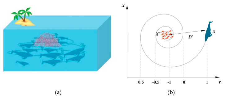
The whale optimization algorithm, which was proposed by Mirjalili and Lewis in 2016, is inspired by the foraging behavior of humpback whales in nature [21]. Humpback whales tend to create spiral bubbles, and then swim to the prey along the trajectory of bubbles (see Figure 1) [25]. The encircling prey and bubble-net attacking behaviors represent the exploitation phase of optimization. The other phase of optimization namely exploration is represented by the search for prey behavior. It is worth noting that the position vector of search agent is defined in a d-dimensional space, where d denotes the number of decision variables of an optimization problem. Thus, the population X of n search agents can be represented by a (n × d)-dimensional matrix, which is shown in Equation (6):
| (6) |
Figure 1.
Bubble-net feeding behavior of humpback whale (a) and the position update model (b).
3.1. Exploitation Phase (Encircling Prey and Bubble-Net Attacking Method)
In the process of hunting, the humpback whales first encircle the prey, which can be represented as follows:
| (7) |
| (8) |
where represents the best solution obtained so far, X denotes the position vector, t is the current iteration, || is the absolute value, · is an element-by-element multiplication, A and C are two essential parameters that can be evaluated by:
| (9) |
| (10) |
where r is a random number in the range of [0,1] and a is a constant that will decrease linearly from 2 to 0 within the whole iterative process (both exploration and exploitation). It can be observed from Equation (8) that search agents can update their position X(t) according the best solution . The parameters A and C determine the distance between the updated position and the optimal position .
The bubble-net attacking behavior can be mathematically represented by the following equation:
| (11) |
| (12) |
where shows the distance between the current search agent position and the optimal position, b is a constant that determine the shape of a logarithmic spiral, and r is a random number in the range of [−1,1]. In order to transform these two mechanisms (encircling prey and bubble-net attacking method) of exploitation phase, assume that each mechanism will be executed with 50% probability. Thus, the mathematical model of the entire exploitation phase can be expressed as:
| (13) |
where p is a random number in the range of [0,1].
3.2. Exploration Phase (Search for Prey)
In order to enhance the exploration capability of algorithm, a global search strategy is utilized. The search agents update their position according to a random agent in the population rather than the best solution obtained so far. It is worth mentioning that the absolute value of A determines the phase of optimization to be selected, namely the exploration and exploitation phases. Thus, the search for prey behavior can be mathematically represented as follows:
| (14) |
| (15) |
where Xrand denotes a random individual in the current population.
Pseudo code of traditional whale optimization algorithm based multilevel thresholding has been given in Algorithm 1.
| Algorithm 1 Pseudo code of whale optimization algorithm based multilevel thresholding |
| Initialize the position of whales Xi. Initialize the best search agent . WHILE t < Maximum number of iterations FOR i = 1:n Calculate the objective value of each search agent by using the Equation (1) for Kapur’s entropy. Update the best search agent . Update a, A, C, r, and p IF1 p < 0.5 IF2 |A| < 1 Update the position of search agent using Equations (7) and (8). ELSE Update the position of search agent using Equations (14) and (15). END IF2 ELSE Update the position of search agent using Equations (11) and (12). END IF1 Correct the position of the current search agent if it is beyond the border. END FOR END WHILE Return , which represents the optimal threshold values of segmentation. |
4. Differential Evolution
Differential evolution (DE) algorithm is a simple and powerful algorithm for solving optimization problems [34,35,36]. Basically, the DE algorithm contains two significant parameters, namely mutation scaling factor denoted by SF and crossover probability denoted by CR [37]. For the standard DE algorithm, the mutation, crossover, and selection operators can be summarized as follows [38]:
4.1. Mutation Operation
The mutation operation of DE algorithm is defined as follows:
| (16) |
where represents the mutant individual in the (g + 1)-th generation. , , and are different individuals from the population. In other words, , , and cannot be equal. SF is a constant that indicates the mutation scaling factor.
4.2. Crossover Operation
In the process of crossover, the trial individual is selected from the current individual or the mutant individual on account of enhancing the diversity of population. The crossover operation of DE algorithm is described as:
| (17) |
where rand represents a random value which is in the range [0,1]. CR is a constant that shows the crossover probability.
4.3. Selection Operation
After the process of selection, the individual of next generation is selected according to the comparison of fitness value between the trail individual and the target individual . For a problem to be minimized, the selection operation of DE algorithm can be summarized as follows:
| (18) |
where f denotes the fitness function value of a given problem.
5. The Proposed Method
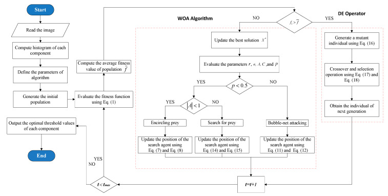
In this section, a detailed introduction of the WOA-DE-based method is given, and the algorithm will be used to obtain the optimal threshold values for image segmentation. A hybrid of the WOA and DE algorithms is introduced to balance the two essential phases of optimization, namely exploration and exploitation. The flowchart of WOA-DE for finding the optimal threshold values is shown in Figure 2.
Figure 2.
Framework of the WOA-DE based method.
It is worth mentioning that a better balance between exploration and exploitation plays an important role in improving the optimization ability of algorithm. Therefore, an efficient hybrid strategy is introduced to balance and improve these two phases. On the one hand, the WOA algorithm has strong ability to explore the solution space and is used as global search technique. On the other hand, the DE algorithm is adopted as local search technique, which can increase the precision of solutions.
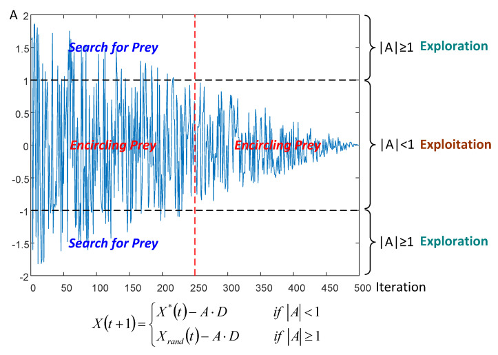
In addition, the purpose of introducing DE operator is not only to enhance the local search ability of the algorithm, but also to overcome the drawback that WOA algorithms easily fall into local optima in the late iterations. As described above, the random variable A will change in the range [−2,2] as a decreases progressively. If the value larger than 1 or less than −1, Equation (15) will be adopted to enhance the exploration capability of the algorithm. On the contrary, Equation (8) will be adopted as local search strategy when the value in the range [−1,1]. In order to more intuitively reflect the change of random variable A during the whole iterative process, a relevant schematic diagram is presented in Figure 3. It can be observed from the figure that the value of random variable A is fixed in the interval of [−1,1] after 250 iterations. This means that the global search strategy has no chance to be adopted after half of the iterative process, even if the current best solution may not the global optimum. Therefore, the traditional WOA algorithm will fall into the local optimum, resulting in an unsatisfactory solution accuracy. Especially for complex multi-dimensional optimization problems, such as multilevel color image segmentation, traditional WOA algorithms cannot handle them. On the contrary, DE operators can scale the difference between any two search agents in the population, which makes the particles jump out of the current search area. In Equation (16), can be considered as the difference between two individuals, and is the scaling factor. The latter term in Equation (16) “” is crucial to the mutation operator. For the exploration stage, particles tend to be very far apart, and there is a big difference between the individuals. Scaling this big difference can enhance the diversity of population. For the exploitation stage, particles tend to be close together, scaling a small difference makes the algorithm effectively optimize in a small range, improving the accuracy of the solution and avoiding local optimum.
Figure 3.
Schematic diagram of the change in random variable A.
In this paper, the average fitness value of the population is computed in the iterative process to evaluate the quality of each particle. The proposed hybrid model enables particles with better quality to exploit the current promising area to ensure the convergence speed, while the particles with poor quality can explore the unknown area to prevent local optimization. Although the global search strategy of traditional WOA algorithm will not be adopted in the later iteration, the introduced DE operator can effectively overcome this shortcoming, as discussed above. Exactly speaking, if , the DE algorithm will be used to update the solution using Equations (16)–(18). However, if , then the current solution will be updated using Equations (8), (12), or (15). In addition, a series of experiments are conducted in the following section to verify the advantages of WOA-DE algorithm from various aspects.
6. Experiments and Results
6.1. Experimental Setup
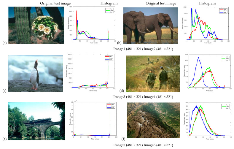
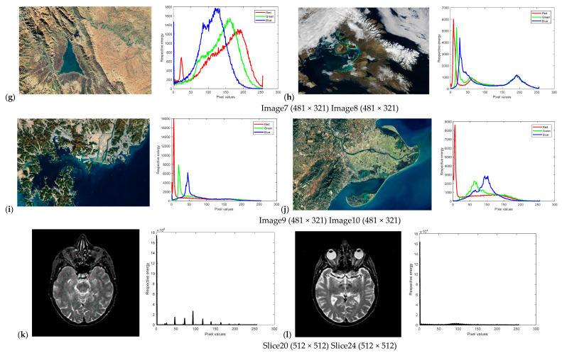
In this paper, Kapur’s entropy thresholding technique is utilized to determine the optimal threshold values for image segmentation. The performance of our WOA-DE-based method is evaluated on fourteen images. Among them, five images are natural images from the Berkeley segmentation database [39], five images are satellite images from [40], and four images are brain magnetic resonance images (MRI) from [41]. Besides, all the images and their corresponding histogram images are shown in Figure 4. Both state-of-the-art and conventional methods, such as the traditional WOA [21], salp swarm algorithm (SSA) [42], sine cosine algorithm (SCA) [43], ant lion optimizer (ALO) [44], harmony search optimization (HSO) [45], bat algorithm (BA) [46], particle swarm optimization (PSO) [47,48], betaDE (BDE) [49], and improved differential search algorithm (IDSA) [50] are used to validate the superiority of proposed algorithm, whose parametric settings are presented in Table 1, except for the population size set to 30 and the number of iterations set to 500 for fair comparison. The experiments are carried out through the simulation in “Matlab2017” (The MathWorks Inc., Natick, MA, USA) and implemented on a computer equipped with the Microsoft Windows 10 operating system and 8 GB memory space.
Figure 4.
Original test images and the corresponding histograms.
Table 1.
Parameters of the algorithms.
6.2. Objective Function Measure
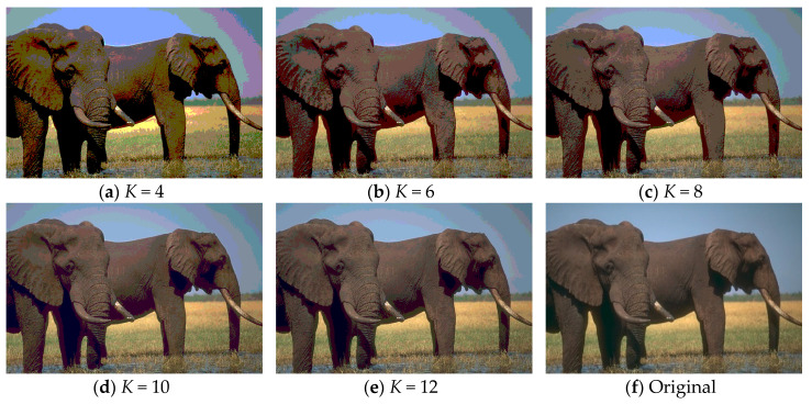
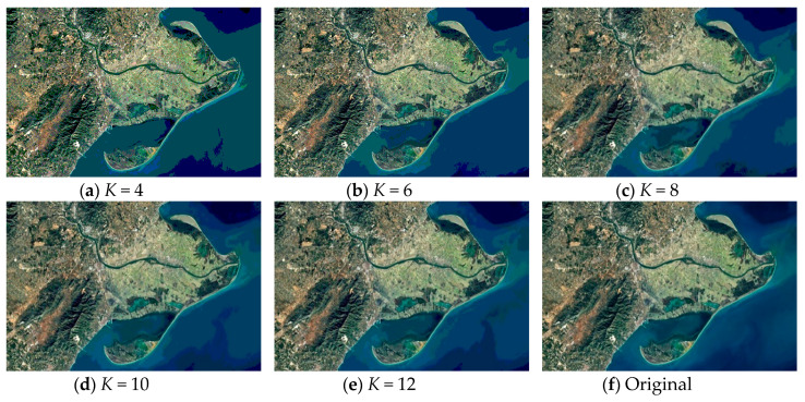
As discussed above, Kapur’s entropy is used to determine the segmentation thresholds. The segmented images of “Image2” and “Image10” obtained by WOA-DE using Kapur’s entropy method with different threshold levels are given in Figure 5 and Figure 6, respectively. Due to the stochastic nature of meta-heuristic algorithms, the experiments are conducted over 30 runs. Then the average objective values of “Image1” and “Image6” are presented in Table 2. It can be seen from the table that the WOA-DE based method gives the best values in general.
Figure 5.
The segmented results of “Image2” at different threshold levels obtained by WOA-DE-Kapur.
Figure 6.
The segmented results of “Image10” at different threshold levels obtained by WOA-DE-Kapur.
Table 2.
The average fitness values and STD values obtained by all algorithms.
| Measures | Image | K | WOA-DE | WOA | SSA | SCA | ALO | HSO | BA | PSO | BDE | IDSA |
|---|---|---|---|---|---|---|---|---|---|---|---|---|
| Mean | Image1 | 4 | 18.5843 | 18.5843 | 18.5843 | 18.5632 | 18.5843 | 18.5761 | 18.5818 | 18.5842 | 18.5843 | 18.5843 |
| 6 | 23.8418 | 23.73 | 23.8408 | 23.479 | 23.8417 | 23.755 | 23.8085 | 23.8412 | 23.8115 | 23.8383 | ||
| 8 | 28.5094 | 28.4605 | 28.5051 | 27.8225 | 28.4627 | 28.385 | 27.7631 | 28.4991 | 28.5118 | 28.5139 | ||
| 10 | 32.8462 | 32.8432 | 32.8325 | 31.3685 | 32.8443 | 32.6682 | 32.0858 | 32.7519 | 32.8455 | 32.7269 | ||
| 12 | 36.8534 | 36.7164 | 36.7269 | 34.5881 | 36.7313 | 36.6221 | 34.7641 | 36.696 | 36.7642 | 36.7764 | ||
| Image6 | 4 | 18.4839 | 18.4784 | 18.4817 | 18.4434 | 18.4836 | 18.4778 | 18.4745 | 18.4839 | 18.4816 | 18.4836 | |
| 6 | 24.0059 | 23.9988 | 23.9994 | 23.765 | 24.005 | 23.9687 | 23.9225 | 24.0015 | 24.0051 | 24.0059 | ||
| 8 | 28.937 | 28.8743 | 28.8836 | 27.9973 | 28.9272 | 28.8508 | 28.2696 | 28.9293 | 28.9342 | 28.9196 | ||
| 10 | 33.3483 | 33.3009 | 33.1851 | 31.8768 | 33.2743 | 33.0867 | 31.6321 | 33.3197 | 33.3079 | 33.2562 | ||
| 12 | 37.3674 | 37.271 | 37.1046 | 35.8876 | 37.3246 | 36.8644 | 35.1068 | 37.1813 | 37.3553 | 37.2569 | ||
| STD | Image1 | 4 | 0 | 2.66 × 10⁻⁵ | 2.66 × 10⁻⁵ | 4.39 × 10⁻³ | 5.83 × 10⁻⁵ | 3.19 × 10⁻³ | 2.17 × 10⁻³ | 2.68 × 10⁻⁵ | 2.47 | 1.58 × 10⁻¹ |
| 6 | 3.25 × 10⁻⁵ | 1.61 × 10⁻⁴ | 9.58 × 10⁻⁴ | 7.45 × 10⁻² | 2.95 × 10⁻⁴ | 1.97 × 10⁻² | 5.39 × 10⁻² | 4.33 × 10⁻⁴ | 8.41 × 10⁻¹ | 1.59 | ||
| 8 | 4.32 × 10⁻⁴ | 2.74 × 10⁻² | 8.89 × 10⁻³ | 1.33 × 10⁻¹ | 3.24 × 10⁻² | 3.38 × 10⁻² | 1.82 × 10⁻¹ | 7.30 × 10⁻³ | 1.3 | 9.98 × 10⁻¹ | ||
| 10 | 3.38 × 10⁻³ | 5.36 × 10⁻³ | 3.90 × 10⁻² | 2.67 × 10⁻¹ | 4.91 × 10⁻² | 3.24 × 10⁻² | 1.51 × 10⁻¹ | 3.34 × 10⁻² | 7.76 × 10⁻¹ | 7.27 × 10⁻¹ | ||
| 12 | 1.83 × 10⁻² | 3.25 × 10⁻² | 7.48 × 10⁻² | 2.30 × 10⁻¹ | 6.12 × 10⁻² | 5.02 × 10⁻² | 6.41 × 10⁻¹ | 7.35 × 10⁻² | 6.66 × 10⁻¹ | 6.65 × 10⁻¹ | ||
| Image6 | 4 | 3.91 × 10⁻³ | 7.91 × 10⁻³ | 4.81 × 10⁻³ | 1.24 × 10⁻² | 8.29 × 10⁻¹ | 5.49 × 10⁻³ | 4.60 × 10⁻³ | 3.93 × 10⁻³ | 6.96 × 10⁻³ | 2.92 × 10⁻¹ | |
| 6 | 1.68 × 10⁻² | 3.81 × 10⁻³ | 1.94 × 10⁻² | 6.82 × 10⁻² | 4.20 × 10⁻³ | 3.58 × 10⁻² | 2.96 × 10⁻² | 5.03 × 10⁻³ | 4.66 | 1.75 | ||
| 8 | 1.57 × 10⁻² | 2.64 × 10⁻² | 1.64 × 10⁻² | 1.60 × 10⁻¹ | 2.48 × 10⁻² | 4.37 × 10⁻² | 3.94 × 10⁻¹ | 6.14 × 10⁻² | 3.88 | 9.82 × 10⁻¹ | ||
| 10 | 2.15 × 10⁻² | 4.26 × 10⁻² | 3.64 × 10⁻² | 1.40 × 10⁻¹ | 5.49 × 10⁻² | 2.50 × 10⁻² | 4.03 × 10⁻¹ | 3.55 × 10⁻² | 2.28 | 8.98 × 10⁻¹ | ||
| 12 | 1.53 × 10⁻² | 3.02 × 10⁻² | 9.90 × 10⁻² | 2.85 × 10⁻¹ | 2.52 × 10⁻² | 6.41 × 10⁻² | 3.37 × 10⁻¹ | 3.43 × 10⁻² | 1.67 | 1.25 |
The entropy of an image reflects its average information content [51]. Therefore, higher value of Kapur’s entropy indicates more information in the image. It can be observed from Table 2 that the objective function value of each algorithm increases with the number of threshold values. This promising result shows that high-quality image with more information is obtained when the threshold level is high (such as K = 10 and 12).
6.3. Stability Analysis
Standard deviation (STD): a value indicates the dispersion of sample data and it is mathematically represented as:
| (19) |
where n is the sample size, fi is the fitness value of the i-th individual, and indicates the average value of the sample.
In order to verify the stability of proposed algorithm, the STD indicator is also used. A lower value of STD indicates better stability. The STD values of “Image1” and “Image6” obtained by all algorithms are presented in Table 2. From the table it is found that WOA-DE based method gives lower values as compared to other algorithms, which shows the better consistency and stability of proposed algorithm.
6.4. Peak Signal to Noise Ratio (PSNR)
Peak signal to noise ratio (PSNR): an index which is used to evaluate the similarity of the processed image against the original image [13]:
| (20) |
represents the mean squared error and is calculated as:
| (21) |
where I(i, j) and K(i, j) denote the gray level of the original image and the segmented image in the i-th row and j-th column, respectively. M and N denote the number of rows and columns in the image matrix, respectively. A higher value of PSNR indicates a better quality segmented image.
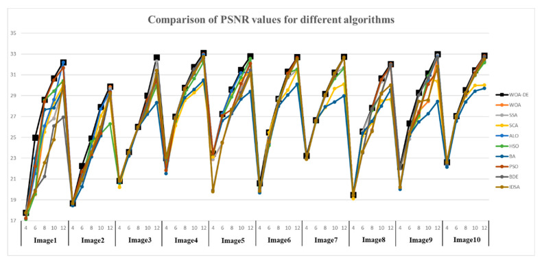
Table 3 shows the PSNR values of “Image2” and “Image7” obtained by all algorithms and Kapur’s entropy method. According to the table, the WOA-DE-based method gives the highest values in 9 out of 10 cases using Kapur’s entropy. When the threshold level is small, all algorithms give similar result, while the obtained values become different as the number of thresholds increases, and the proposed method can present the best result in most cases. This phenomenon indicates that WOA-DE-based method can determine the appropriate thresholds and then present high-quality segmented image that are more similar to the original image. Figure 7 shows the visual comparison of all available methods at different threshold levels. The results of proposed method are represented as “black” lines and “square” data points.
Table 3.
The PSNR, SSIM, and FSIM values obtained by all algorithms under different threshold levels.
| Measures | Image | K | WOA-DE | WOA | SSA | SCA | ALO | HSO | BA | PSO | BDE | IDSA |
|---|---|---|---|---|---|---|---|---|---|---|---|---|
| PSNR | Image2 | 4 | 18.6558 | 18.6558 | 18.6558 | 18.6533 | 18.6558 | 18.5722 | 18.4352 | 18.6558 | 18.6452 | 18.6558 |
| 6 | 22.2481 | 20.8588 | 21.3402 | 21.5799 | 21.3148 | 20.861 | 20.2596 | 21.7136 | 20.8588 | 20.9995 | ||
| 8 | 24.8821 | 23.1744 | 23.6373 | 23.4877 | 24.1624 | 24.5724 | 23.1158 | 23.372 | 23.5863 | 23.5837 | ||
| 10 | 27.9116 | 25.3956 | 25.9502 | 27.0446 | 27.7051 | 25.3211 | 25.1289 | 25.3938 | 25.87 | 25.9861 | ||
| 12 | 29.8805 | 29.8395 | 29.6719 | 28.6767 | 29.4309 | 26.3023 | 29.2218 | 29.34 | 29.0663 | 29.2001 | ||
| Image7 | 4 | 23.2367 | 22.947 | 22.9286 | 22.9305 | 23.0442 | 22.9765 | 22.923 | 22.982 | 22.982 | 22.9122 | |
| 6 | 26.6481 | 26.5553 | 26.5205 | 26.5953 | 26.656 | 26.4685 | 26.5963 | 26.6156 | 26.527 | 26.5732 | ||
| 8 | 29.1886 | 29.1004 | 28.9405 | 27.8606 | 29.132 | 29.063 | 27.9378 | 29.0088 | 29.1151 | 29.0763 | ||
| 10 | 31.2154 | 30.9433 | 31.1186 | 29.6665 | 30.9579 | 30.64 | 28.3997 | 30.9199 | 31.0374 | 31.169 | ||
| 12 | 32.7203 | 32.6538 | 31.7022 | 30.101 | 32.6566 | 31.6295 | 28.988 | 32.7035 | 32.6774 | 32.6603 | ||
| SSIM | Image2 | 4 | 0.5266 | 0.5266 | 0.5266 | 0.5253 | 0.5186 | 0.5212 | 0.5212 | 0.5266 | 0.5242 | 0.5266 |
| 6 | 0.652 | 0.6103 | 0.617 | 0.6105 | 0.6192 | 0.6379 | 0.5864 | 0.6332 | 0.6103 | 0.6197 | ||
| 8 | 0.7361 | 0.6944 | 0.7052 | 0.6976 | 0.7281 | 0.7224 | 0.7094 | 0.6978 | 0.7004 | 0.6963 | ||
| 10 | 0.8064 | 0.7551 | 0.7608 | 0.7701 | 0.7996 | 0.7534 | 0.7247 | 0.7594 | 0.7705 | 0.7733 | ||
| 12 | 0.8505 | 0.8484 | 0.8432 | 0.7859 | 0.8411 | 0.8463 | 0.8182 | 0.8367 | 0.8483 | 0.8269 | ||
| Image7 | 4 | 0.8494 | 0.8414 | 0.8407 | 0.8419 | 0.8456 | 0.8405 | 0.8382 | 0.8416 | 0.8416 | 0.8399 | |
| 6 | 0.9136 | 0.9097 | 0.907 | 0.9086 | 0.9115 | 0.9091 | 0.9098 | 0.9087 | 0.9091 | 0.9079 | ||
| 8 | 0.9422 | 0.9409 | 0.9392 | 0.9254 | 0.9415 | 0.9412 | 0.9241 | 0.9404 | 0.9416 | 0.9418 | ||
| 10 | 0.9648 | 0.9608 | 0.9603 | 0.946 | 0.9587 | 0.9552 | 0.9255 | 0.9624 | 0.9633 | 0.9637 | ||
| 12 | 0.9726 | 0.9715 | 0.9624 | 0.9543 | 0.9724 | 0.963 | 0.9338 | 0.9718 | 0.9724 | 0.9725 | ||
| FSIM | Image2 | 4 | 0.7151 | 0.7151 | 0.7151 | 0.7149 | 0.7151 | 0.7117 | 0.7115 | 0.7151 | 0.7142 | 0.7151 |
| 6 | 0.7921 | 0.7707 | 0.7723 | 0.7708 | 0.7711 | 0.7876 | 0.7577 | 0.7799 | 0.7707 | 0.7866 | ||
| 8 | 0.8435 | 0.8257 | 0.8289 | 0.8246 | 0.8426 | 0.8313 | 0.8093 | 0.824 | 0.8256 | 0.8198 | ||
| 10 | 0.8745 | 0.8617 | 0.8582 | 0.8423 | 0.8738 | 0.8616 | 0.8153 | 0.864 | 0.8686 | 0.8682 | ||
| 12 | 0.9041 | 0.9036 | 0.9005 | 0.8987 | 0.9007 | 0.8978 | 0.8531 | 0.8806 | 0.9022 | 0.8915 | ||
| Image7 | 4 | 0.9012 | 0.8964 | 0.8959 | 0.8965 | 0.8991 | 0.8968 | 0.8953 | 0.8972 | 0.8972 | 0.8956 | |
| 6 | 0.9469 | 0.9445 | 0.946 | 0.9458 | 0.9467 | 0.9449 | 0.9468 | 0.9465 | 0.9453 | 0.9464 | ||
| 8 | 0.9671 | 0.9666 | 0.9658 | 0.9591 | 0.9665 | 0.9659 | 0.9559 | 0.9658 | 0.9666 | 0.966 | ||
| 10 | 0.9773 | 0.9758 | 0.9752 | 0.971 | 0.9759 | 0.9754 | 0.9574 | 0.9765 | 0.9761 | 0.9763 | ||
| 12 | 0.9834 | 0.9824 | 0.9799 | 0.9729 | 0.9829 | 0.9802 | 0.9664 | 0.9828 | 0.9825 | 0.9826 |
Figure 7.
Comparison of PSNR values for different algorithms using Kapur’s entropy at 4, 6, 8, 10, and 12 levels.
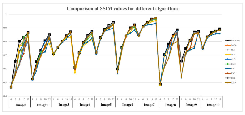
6.5. Structural Similarity Index (SSIM)
Structural similarity index (SSIM) [52,53]: a measure of the similarity between the original image and the segmented image, which takes various factors such as brightness, contrast, and structural similarity into account:
| (22) |
where and denote the mean intensities of the original image and the segmented image respectively. and are the standard deviation of the original image and the segmented image respectively. denotes the covariance between the original image and the segmented image. and are constants. The value of SSIM is in the range [0,1], and a higher value shows better performance.
The SSIM values obtained by all algorithms are given in Table 3 and Figure 8, respectively. It can be seen from the table that the WOA-DE-based method gives competitive results again compared with other methods in terms of SSIM indicator. The values obtained by all algorithms increase with the number of thresholds, which indicates that the segmented image is more similar to the original image in terms of brightness, contrast, and structural similarity. The experimental results in this section verify the remarkable performance of the proposed algorithm from another perspective.
Figure 8.
Comparison of SSIM values for different algorithms using Kapur’s entropy at 4, 6, 8, 10, and 12 levels.
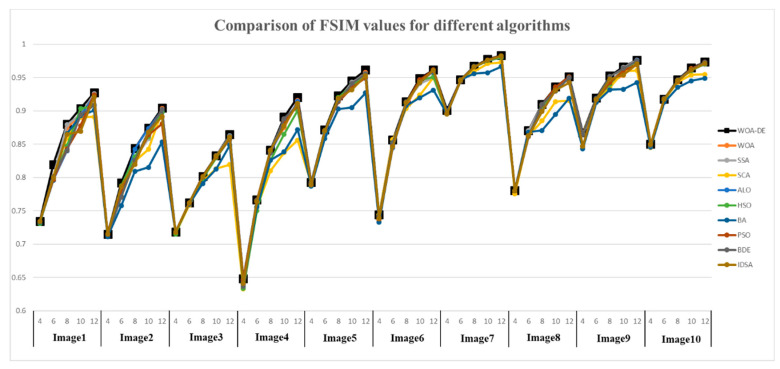
6.6. Feature Similarity Index (FSIM)
Feature similarity index (FSIM) [54,55]: another measure of the image quality through evaluating the feature similarity between the original image and the segmented image:
| (23) |
where Ω represents the whole image pixel domain. is a similarity score. denotes the phase consistency measure, which is defined as:
| (24) |
where and represent the phase consistency of two blocks, respectively:
| (25) |
| (26) |
| (27) |
denotes the similarity measure of phase consistency. denotes the gradient magnitude of two regions and . , , , and are all constants. The value of FSIM is also in the range [0,1], and a higher value shows better segmented image quality.
On comparing the FSIM values, which are given in Table 3 and Figure 9, it can be observed that WOA-DE-based method again outperforms the other methods. The feature similarity between the original image and the segmented image is considered in this experiment to verify the quality of segmented image comprehensively. The relevant results indicate that the proposed method has a strong feature preserving ability as compared to other methods.
Figure 9.
Comparison of FSIM values for different algorithms using Kapur’s entropy at 4, 6, 8, 10, and 12 levels.
6.7. Convergence Performance
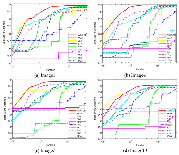
In this section, the convergence performance of all algorithms is evaluated and discussed in details. In order to reflect the performance of WOA-DE more intuitively, the convergence curves of Kapur’s entropy function (for K = 12) are shown in Figure 10. Four different images are selected for testing, namely “Image1”, “Image4”, “Image7”, and “Image10”. It can be found that the proposed algorithm outperforms other algorithms in general. In other words, the WOA-DE-based method gives higher position curves using Kapur’s entropy technique.
Figure 10.
The convergence curves for fitness function using Kapur’s entropy method at 12 levels thresholding.
As discussed above, the main drawbacks of the standard WOA are premature convergence and unbalanced exploration-exploitation, which are clearly reflected in the curves. For example, under the circumstance of “Image1” segmentation, the objective function value of WOA is almost never updated after 100 iterations, while the optimal value obtained is not the best. This phenomenon illustrates the premature convergence shortcoming of WOA. However, the proposed WOA-DE algorithm gives the highest objective function value under the premise of ensuring the convergence speed. In fact, the remarkable performance of the proposed algorithm is not only reflected in the segmentation task of “Image1”, but also in other images. The experimental results in this section indicate that WOA-DE algorithm can better balance the exploration and exploitation, and the complex image segmentation tasks are also competent.
6.8. Computation Time
The average CPU time of different algorithms considering all cases is given in Table 4. It can be found from the table that HSO is the fastest among available methods, but the segmentation accuracy discussed above is not ideal. The standard WOA algorithm gives competitive results in some cases, and the proposed algorithm namely WOA-DE is slightly slower than the standard WOA. The reason for this phenomenon is the premature convergence of HSO algorithm, which cannot well balance exploration and exploitation. On the contrary, the WOA-DE algorithm combines the advantages of both WOA and DE, which determine the most appropriate threshold value, despite not being the fastest. To sum up, WOA-DE is a high-performance hybrid algorithm that improves segmentation precision while maintaining runtime.
Table 4.
The average computation time (s) considering all images under different threshold levels.
| K | WOA-DE | WOA | SSA | SCA | ALO | HSO | BA | PSO | BDE | IDSA |
|---|---|---|---|---|---|---|---|---|---|---|
| 4 | 1.40087 | 1.047 | 1.49062 | 1.49438 | 7.8046 | 1.03739 | 1.97122 | 1.70887 | 2.21335 | 1.41216 |
| 6 | 1.55259 | 1.14527 | 1.63902 | 1.62171 | 9.66773 | 1.10338 | 2.08452 | 1.88491 | 2.40389 | 1.5397 |
| 8 | 1.67041 | 1.18449 | 1.72857 | 1.6764 | 12.09074 | 1.18478 | 2.31804 | 1.99103 | 2.48257 | 1.56885 |
| 10 | 1.74287 | 1.24446 | 1.79294 | 1.86849 | 15.31865 | 1.23933 | 2.36836 | 2.13532 | 2.58595 | 1.67435 |
| 12 | 1.88104 | 1.39335 | 1.95442 | 1.98369 | 17.19651 | 1.30339 | 2.513 | 2.23487 | 2.74791 | 1.70745 |
6.9. Statistical Analysis
In this section, a non-parametric statistical test known as “Wilcoxon’s rank sum test” is used to evaluate the significant difference between algorithms [56]. The experiments are conducted 30 runs at significance level 5%. All experimental data obtained based on Kapur’s entropy are used for testing. The alternative hypothesis assumes that there is a significant difference between the two algorithms being compared. The null hypothesis considers that there is no significant difference between the algorithms. The results of the statistical experiments are given in Table 5.
Table 5.
Wilcoxon’s rank sum test results.
| Comparison | p-Value |
|---|---|
| WOA-DE versus WOA | 2.3197 × 10⁻⁴ |
| WOA-DE versus SSA | 9.0193 × 10⁻⁸ |
| WOA-DE versus SCA | 6.8546 × 10⁻⁷ |
| WOA-DE versus ALO | 4.2264 × 10⁻¹⁰ |
| WOA-DE versus HSO | 7.6791 × 10⁻⁷ |
| WOA-DE versus BA | 3.2115 × 10⁻⁹ |
| WOA-DE versus PSO | 7.6473 × 10⁻⁸ |
| WOA-DE versus BDE | 4.5474 × 10⁻⁵ |
| WOA-DE versus IDSA | 7.0546 × 10⁻⁴ |
It can be observed from the table that the p-values acquired are far less than 0.05. This promising result indicates that can be rejected in all cases and there is a significant difference between the proposed algorithm and other methods.
6.10. Comparison of Otsu and Kapur’s Entropy Methods
In order to obtain a simple and powerful technique for color image segmentation, an experiment of comparison between Otsu and Kapur’s entropy thresholding techniques based on WOA-DE is conducted in this section. More details of Otsu thresholding technique can be found in [11].
The PSNR, SSIM, and FSIM values obtained by WOA-DE-based method are given in Table 6. It can be seen that WOA-DE-based method using Kapur’s entropy gives higher values than using Otsu technique in general for PSNR values. However, the Otsu-based technique performs better when comparing SSIM values. Considering the FSIM indicator, these two thresholding techniques are equal. Precisely speaking, on comparing the PSNR values, the Otsu technique presents better results in 11 out of 50 cases (10 images and five thresholds), whereas, Kapur’s entropy technique gives better results in 39 out of 50 cases. Considering other two indicators, the Kapur’s entropy technique outperforms in 21 cases for SSIM and 25 cases for FSIM, while the Otsu technique outperforms in 29 cases for SSIM and 25 cases for FSIM. To sum up, the WOA-DE-based method through Otsu gives better results in 65 out of 150 cases (10 images, five thresholds, and three performance measures) and the WOA-DE-based method through Kapur’s entropy gives satisfactory results in 85 cases. To some extent, these satisfactory results prove that WOA-DE-based method using Kapur’s entropy is superior to the method using Otsu. However, as the no free lunch (NFL) theorem goes, there is no technique that can handle all image segmentation tasks [57]. Thus, the WOA-DE algorithm based on different thresholding techniques has potential in the field of color image segmentation, which may exhibit superior performance in some engineering problems that have not been solved so far.
Table 6.
Comparison of Kapur’s entropy and Otsu methods based on WOA-DE algorithm.
| Images | K | PSNR | SSIM | FSIM | |||
|---|---|---|---|---|---|---|---|
| Otsu | Kapur | Otsu | Kapur | Otsu | Kapur | ||
| Image1 | 4 | 20.3428 | 17.7781 | 0.5798 | 0.4681 | 0.7771 | 0.734 |
| 6 | 22.6702 | 24.977 | 0.6815 | 0.6559 | 0.8458 | 0.8197 | |
| 8 | 24.0516 | 28.6092 | 0.7446 | 0.8033 | 0.9122 | 0.8798 | |
| 10 | 25.2164 | 30.6687 | 0.7898 | 0.833 | 0.9225 | 0.9039 | |
| 12 | 26.1897 | 32.2054 | 0.8059 | 0.8672 | 0.926 | 0.9271 | |
| Image2 | 4 | 18.459 | 18.6558 | 0.608 | 0.5266 | 0.7582 | 0.7151 |
| 6 | 20.9182 | 22.2481 | 0.7095 | 0.652 | 0.8245 | 0.7921 | |
| 8 | 24.5622 | 24.8821 | 0.8164 | 0.7361 | 0.8684 | 0.8435 | |
| 10 | 25.7585 | 27.9116 | 0.8421 | 0.8064 | 0.8878 | 0.8745 | |
| 12 | 28.4144 | 29.8805 | 0.8964 | 0.8505 | 0.917 | 0.9041 | |
| Image3 | 4 | 17.5776 | 20.8247 | 0.6971 | 0.7109 | 0.6972 | 0.7182 |
| 6 | 22.7555 | 23.6059 | 0.7431 | 0.7592 | 0.7469 | 0.7619 | |
| 8 | 27.8967 | 26.0132 | 0.7948 | 0.8036 | 0.795 | 0.8017 | |
| 10 | 29.5405 | 29.0184 | 0.8341 | 0.8433 | 0.8322 | 0.8329 | |
| 12 | 31.6891 | 32.6886 | 0.8633 | 0.8729 | 0.8619 | 0.8646 | |
| Image4 | 4 | 19.0015 | 23.013 | 0.6151 | 0.612 | 0.7012 | 0.6484 |
| 6 | 24.4296 | 26.9872 | 0.7631 | 0.7188 | 0.8129 | 0.7665 | |
| 8 | 27.9781 | 29.7682 | 0.8434 | 0.7953 | 0.8793 | 0.8415 | |
| 10 | 32.0713 | 31.7603 | 0.8888 | 0.8456 | 0.9193 | 0.8907 | |
| 12 | 33.9227 | 33.096 | 0.9194 | 0.8767 | 0.9431 | 0.9203 | |
| Image5 | 4 | 23.4509 | 23.4495 | 0.8082 | 0.7231 | 0.8469 | 0.7925 |
| 6 | 27.2396 | 27.2417 | 0.8948 | 0.8286 | 0.9142 | 0.8716 | |
| 8 | 29.6073 | 29.5852 | 0.926 | 0.8903 | 0.9415 | 0.9229 | |
| 10 | 31.5024 | 31.4704 | 0.9345 | 0.919 | 0.9585 | 0.9452 | |
| 12 | 32.9105 | 32.782 | 0.9457 | 0.9429 | 0.9672 | 0.9614 | |
| Image6 | 4 | 19.2192 | 20.597 | 0.6626 | 0.5995 | 0.7712 | 0.7443 |
| 6 | 23.4934 | 25.4883 | 0.8061 | 0.7587 | 0.8673 | 0.8562 | |
| 8 | 27.6467 | 28.6898 | 0.8732 | 0.8427 | 0.9192 | 0.9136 | |
| 10 | 29.7289 | 31.292 | 0.9104 | 0.9002 | 0.9416 | 0.9489 | |
| 12 | 32.0406 | 32.7058 | 0.9384 | 0.9227 | 0.9599 | 0.9615 | |
| Image7 | 4 | 18.9474 | 23.2367 | 0.7898 | 0.8494 | 0.848 | 0.9012 |
| 6 | 23.6742 | 26.6481 | 0.8938 | 0.9136 | 0.9198 | 0.9469 | |
| 8 | 26.8294 | 29.1886 | 0.9383 | 0.9422 | 0.9513 | 0.9671 | |
| 10 | 30.559 | 31.2154 | 0.9626 | 0.9648 | 0.9728 | 0.9773 | |
| 12 | 32.9021 | 32.7203 | 0.9781 | 0.9726 | 0.9828 | 0.9834 | |
| Image8 | 4 | 20.3695 | 19.4801 | 0.5372 | 0.4881 | 0.786 | 0.7807 |
| 6 | 23.4982 | 25.5717 | 0.6365 | 0.7043 | 0.8643 | 0.8705 | |
| 8 | 25.5399 | 27.8173 | 0.7326 | 0.7823 | 0.9007 | 0.9102 | |
| 10 | 27.2326 | 30.6727 | 0.8174 | 0.8479 | 0.9228 | 0.9361 | |
| 12 | 30.4945 | 32.0442 | 0.8483 | 0.8849 | 0.943 | 0.9514 | |
| Image9 | 4 | 20.5858 | 22.1696 | 0.6759 | 0.6581 | 0.8498 | 0.8671 |
| 6 | 25.1403 | 26.3449 | 0.7465 | 0.7492 | 0.9174 | 0.9197 | |
| 8 | 28.672 | 29.2954 | 0.7938 | 0.8082 | 0.9476 | 0.9524 | |
| 10 | 30.9026 | 31.126 | 0.8711 | 0.8716 | 0.9664 | 0.9661 | |
| 12 | 32.5855 | 32.9878 | 0.9012 | 0.8757 | 0.9761 | 0.9764 | |
| Image10 | 4 | 20.2121 | 22.6128 | 0.7399 | 0.7551 | 0.8312 | 0.8499 |
| 6 | 24.9168 | 27.0397 | 0.8128 | 0.8355 | 0.9075 | 0.9179 | |
| 8 | 29.1254 | 29.5441 | 0.8865 | 0.8649 | 0.9503 | 0.947 | |
| 10 | 30.9532 | 31.447 | 0.9196 | 0.8774 | 0.9641 | 0.9645 | |
| 12 | 32.5129 | 32.8351 | 0.9284 | 0.8923 | 0.9729 | 0.9734 | |
| Rank | 2(11) | 1(39) | 2(29) | 1(21) | 1(25) | 1(25) | |
6.11. Robustness Testing on Noisy Images
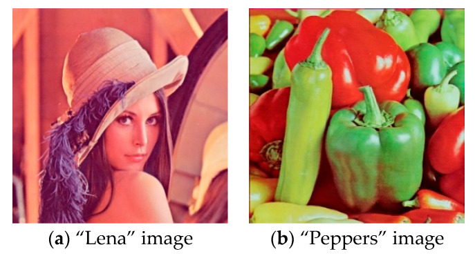
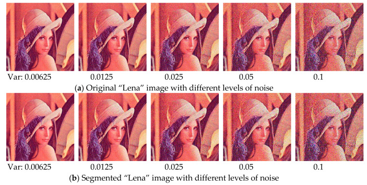
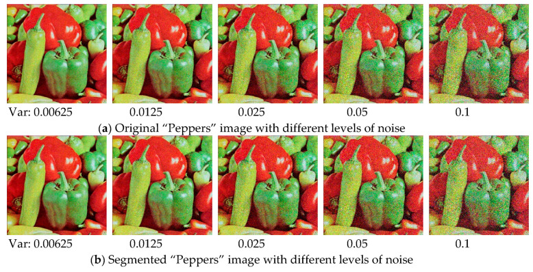
In order to further investigate the performance of proposed algorithm, an experiment is conducted on two famous benchmark test images with various noise levels. “Lena” and “Peppers” images are used in this section (see Figure 11), which can be obtained from [58]. The mean value is fixed in this experiment, and the level of Gaussian noise is adjusted by setting the variance as 0.00625, 0.0125, 0.025, 0.05, and 0.1, respectively. The experiment is carried out at 12 threshold level, in which case the difference between algorithms is the most obvious. The relevant results are presented in Figure 12, Figure 13, Figure 14 and Figure 15. It can be observed from the results that the value of performance measures and quality of segmented image decrease with the increase of noise level, and the WOA-DE-Kapur outperforms other methods using Kapur entropy. The promising results indicate that the proposed technique has strong robustness, which can be competent for complex image segmentation tasks with noise.
Figure 11.
Original “Lena” and “Peppers” images from Berkeley Segmentation Dataset.
Figure 12.
The original “Lena” image and the corresponding segmented results under various noise levels.
Figure 13.
The original “Peppers” image and the corresponding segmented results under various noise levels.
Figure 14.
The value of various performance measures over “Lena” image with different levels of noise.
Figure 15.
The value of various performance measures over “Peppers” image with different levels of noise.
6.12. Application in MR Image
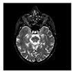
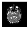
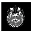
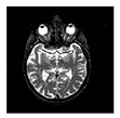
In this section, the WOA-DE-Kapur-based multilevel thresholding technique is applied to the field of MR image segmentation. The purpose of this experiment is to investigate whether the proposed algorithm is capable of producing high quality segmented MR images. Two other threshold-based MR image segmentation techniques are used for comparison, namely the crow search algorithm-based method using minimum cross entropy thresholding (CSA-MCET) [59] and adaptive bacterial foraging algorithm-based method using Otsu (ABF-Otsu) [60]. The combination of thresholds (K = 2, 3, 4, and 5) selected is the same as that used by above two algorithms in their corresponding articles. Besides, the parameter values are set according to the original literature, except for the population size set to 30 and the number of iterations set to 500 for fair comparison. All experiments are performed 30 times to eliminate errors.
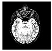
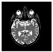
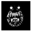
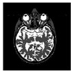
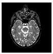
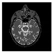
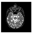
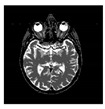
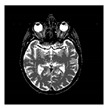
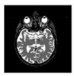
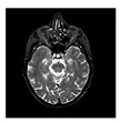
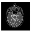
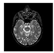
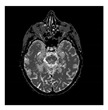
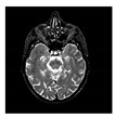
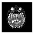
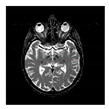
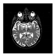
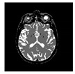
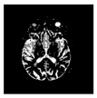
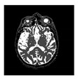
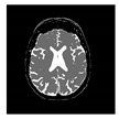
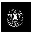
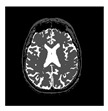
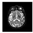
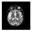
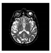
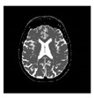
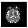
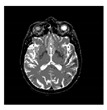
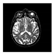
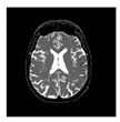
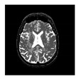
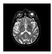
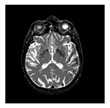
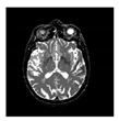
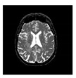
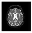
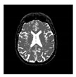
The experimental results are shown in three tables. Table 7 presents the optimal thresholds and PSNR values, Table 8 gives the SSIM and FSIM values, and Table 9 indicates the segmented images obtained by all methods. It can be found from these results that WOA-DE-Kapur method can determine more accurate thresholds compared to other methods. For quantitative analysis, the values of performance measures obtained by proposed method is higher, which indicate the better quality of segmented image. For visual analysis, WOA-DE-Kapur method gives more informative segmented MR images, and the details of image become more prominent as the number of thresholds increases.
Table 7.
Comparison of Optimal threshold and PSNR value obtained by WOA-DE-Kapur, ABF-Otsu, and CSA-MCET.
| Images | K | Optimal Threshold Value | PSNR | ||||
|---|---|---|---|---|---|---|---|
| WOA-DE-Kapur | ABF-Otsu | CSA-MCET | WOA-DE-Kapur | ABF-Otsu | CSA-MCET | ||
| Slice20 | 2 | 94 167 | 28 97 | 13 84 | 16.8586 | 16.524 | 15.9746 |
| 3 | 9 118 219 | 29 87 151 | 18 64 134 | 23.9008 | 23.1061 | 22.4605 | |
| 4 | 8 29 129 210 | 7 53 100 153 | 16 64 98 147 | 24.6228 | 25.4972 | 24.3967 | |
| 5 | 16 36 94 171 211 | 21 54 98 156 190 | 3 40 61 113 150 | 30.4912 | 27.3411 | 28.5034 | |
| Slice24 | 2 | 111 182 | 48 145 | 19 118 | 19.7345 | 21.0839 | 20.8004 |
| 3 | 34 117 182 | 40 108 172 | 7 56 136 | 23.4428 | 22.9913 | 23.5030 | |
| 4 | 17 73 129 193 | 23 70 118 182 | 6 50 101 161 | 26.7848 | 26.2061 | 24.7095 | |
| 5 | 14 70 115 165 210 | 20 63 102 143 196 | 4 27 66 111 170 | 28.9204 | 28.3318 | 25.3871 | |
| Slice28 | 2 | 114 179 | 52 151 | 20 121 | 19.6991 | 18.6884 | 19.1865 |
| 3 | 20 81 156 | 46 110 175 | 7 56 139 | 24.8983 | 24.3616 | 23.7032 | |
| 4 | 22 78 137 192 | 27 76 126 187 | 6 48 103 161 | 26.9455 | 27.0419 | 25.8075 | |
| 5 | 13 72 117 157 203 | 23 68 109 149 203 | 6 36 74 115 174 | 29.6822 | 29.1884 | 28.1382 | |
| Slice32 | 2 | 115 175 | 53 159 | 20 137 | 23.3496 | 22.888 | 22.6576 |
| 3 | 16 76 143 | 50 120 189 | 8 54 148 | 24.711 | 23.2735 | 25.9537 | |
| 4 | 16 74 131 186 | 21 70 122 191 | 7 52 107 172 | 27.5852 | 27.958 | 27.947 | |
| 5 | 18 71 118 162 205 | 19 63 105 147 206 | 3 28 67 116 180 | 29.7914 | 28.6183 | 29.598 | |
| Rank | — | — | — | 1(10) | 2(4) | 3(2) | |
Table 8.
Comparison of SSIM and FSIM value obtained by WOA-DE-Kapur, ABF-Otsu, and CSA-MCET.
| Images | K | SSIM | FSIM | ||||
|---|---|---|---|---|---|---|---|
| WOA-DE-Kapur | ABF-Otsu | CSA-MCET | WOA-DE-Kapur | ABF-Otsu | CSA-MCET | ||
| Slice20 | 2 | 0.7923 | 0.7726 | 0.7882 | 0.8743 | 0.8565 | 0.8421 |
| 3 | 0.8784 | 0.8061 | 0.8811 | 0.9411 | 0.9305 | 0.9594 | |
| 4 | 0.9225 | 0.8408 | 0.9208 | 0.9608 | 0.9614 | 0.9599 | |
| 5 | 0.9435 | 0.8862 | 0.9249 | 0.9882 | 0.9674 | 0.9723 | |
| Slice24 | 2 | 0.6809 | 0.7886 | 0.7865 | 0.7772 | 0.8178 | 0.8117 |
| 3 | 0.8391 | 0.8318 | 0.8343 | 0.8686 | 0.8660 | 0.8394 | |
| 4 | 0.8791 | 0.8770 | 0.8742 | 0.9081 | 0.9026 | 0.8944 | |
| 5 | 0.9015 | 0.8959 | 0.8997 | 0.9277 | 0.9253 | 0.9099 | |
| Slice28 | 2 | 0.7832 | 0.7678 | 0.7792 | 0.813 | 0.8394 | 0.8274 |
| 3 | 0.8365 | 0.8238 | 0.8275 | 0.8849 | 0.8846 | 0.8585 | |
| 4 | 0.8672 | 0.8687 | 0.8691 | 0.9084 | 0.9136 | 0.9156 | |
| 5 | 0.8993 | 0.8937 | 0.9010 | 0.9371 | 0.9355 | 0.9366 | |
| Slice32 | 2 | 0.8123 | 0.7973 | 0.7862 | 0.8617 | 0.8388 | 0.8589 |
| 3 | 0.8465 | 0.832 | 0.8513 | 0.8864 | 0.8943 | 0.9009 | |
| 4 | 0.8794 | 0.8824 | 0.8784 | 0.9199 | 0.9271 | 0.9275 | |
| 5 | 0.9023 | 0.8705 | 0.8991 | 0.9477 | 0.9237 | 0.9347 | |
| Rank | 1(10) | 3(2) | 2(4) | 1(9) | 3(3) | 2(4) | |
Table 9.
The segmented MRI for different algorithms at 2, 3, 4, and 5 levels.
| K | WOA-DE-Kapur | ABF-Otsu | CSA-MCET | WOA-DE-Kapur | ABF-Otsu | CSA-MCET |
|---|---|---|---|---|---|---|
| Slice20 | Slice24 | |||||
| 2 |
|
|
|
|
|
|
| 3 |
|
|
|
|
|
|
| 4 |
|
|
|
|
|
|
| 5 |
|
|
|
|
|
|
| K | Slice28 | Slice32 | ||||
| 2 |
|
|
|
|
|
|
| 3 |
|
|
|
|

|

|
| 4 |
|
|
|
|

|
|
| 5 |
|
|
|
|
|
|
Since the experiments of three methods are the same, it is necessary to carry out relevant statistical tests. In this section, Friedman test [61] and Wilcoxon’s rank sum test [56] are used as non-parametric statistical test to evaluate the performance of these methods considering 5% as significant level. Null hypothesis in Friedman test states equality of medians between the algorithms, and the alternative hypothesis indicates the difference. A more detailed description of Friedman test can be found in literature [62]. The results of the relevant statistical tests can be observed in Table 10 and Table 11. Table 10 presents the average rank and p-value of all algorithms at different threshold levels. As can be found, ABF-Otsu obtains the first rank for K = 3, and WOA-DE-Kapur provides the first rank in other cases. In other words, the proposed technique gives the best result in general. The p-value for all threshold levels is very small indicating the significant difference among available methods. Table 11 gives the result of Wilcoxon’s rank sum test. It can be observed that the p-value is less than 0.05 in most cases, which verifies the remarkable performance of WOA-DE-Kapur technique in a statistical and meaningful way.
Table 10.
Friedman test for WOA-DE-Kapur, ABF-Otsu, and CSA-MCET on MR images.
| K | Average Rank | p-Value | ||
|---|---|---|---|---|
| WOA-DE-Kapur | ABF-Otsu | CSA-MCET | ||
| 2 | 1.6667 | 2.0000 | 2.3333 | 2.2619 × 10⁻⁷ |
| 3 | 1.5833 | 2.5833 | 1.8333 | 1.1603 × 10⁻⁸ |
| 4 | 2.0000 | 1.6667 | 2.3333 | 7.2217 × 10⁻⁹ |
| 5 | 1.0833 | 2.7500 | 2.1667 | 5.3467 × 10⁻⁹ |
Table 11.
Wilcoxon’s rank sum test for WOA-DE-Kapur, ABF-Otsu, and CSA-MCET on MR images.
| K | WOA-DE-Kapur vs. ABF-Otsu | WOA-DE-Kapur vs. CSA-MCET | ||
|---|---|---|---|---|
| p-Value | h | p-Value | h | |
| 2 | < 0.05 | 1 | < 0.05 | 1 |
| 3 | < 0.05 | 1 | 0.0926 | 0 |
| 4 | < 0.05 | 1 | < 0.05 | 1 |
| 5 | < 0.05 | 1 | < 0.05 | 1 |
7. Conclusions
In order to obtain an efficient technique for color image segmentation, an improved WOA-based method is introduced in this paper, which is known as WOA-DE. In the proposed algorithm, DE is adopted as a local search strategy with the purpose of enhancing exploitation capability. Compared to the traditional WOA, the WOA-DE algorithm can effectively avoid falling into a local optimum and prevent the loss of population diversity in the later iterations. A series of experiments have been conducted on various color images including natural images and satellite images. Seven meta-heuristic algorithms are utilized for comparison. The experimental results indicate that the proposed techniques outperform other methods in terms of average fitness values, standard deviation (STD), peak signal to noise ratio (PSNR), structural similarity index (SSIM), and feature similarity index (FSIM) as well as the Wilcoxon’s rank sum test. In addition, to give more convincing and reliable results, another thresholding technique namely Otsu is adopted for testing. The experimental results indicate that WOA-DE-based technique through Kapur’s entropy gives better results than using the Otsu technique in most cases. However, there is no technique that can handle all image segmentation tasks. Thus, it is necessary to introduce more and better techniques to meet the requirements of different image segmentation problems and this is also the motivation for our future research. The performance of some novel meta-heuristic algorithms will be evaluated in this domain, such as salp swarm algorithm, spotted hyena optimizer, emperor penguin optimizer, etc.
Acknowledgments
The authors would like to thank the anonymous reviewers for their constructive comments and suggestions.
Author Contributions
C.L. and H.J. contributed to the idea of this paper; C.L. performed the experiments; C.L. wrote the paper; C.L. and H.J. contributed to the revision of this paper.
Funding
This research received no external funding.
Conflicts of Interest
The authors declare no conflict of interest.
References
- 1.Qian P., Zhao K., Jiang Y., Su K., Deng Z., Wang S., Muzic R.F. Knowledge-leveraged transfer fuzzy C-Means for texture image segmentation with self-adaptive cluster prototype matching. Knowl.-Based Syst. 2017;130:33–50. doi: 10.1016/j.knosys.2017.05.018. [DOI] [PMC free article] [PubMed] [Google Scholar]
- 2.Robert M., Carsten M., Olivier E., Jochen P., Noordhoek N.J., Aravinda T., Reddy V.Y., Chan R.C., Jürgen W. Automatic Segmentation of Rotational X-Ray Images for Anatomic Intra-Procedural Surface Generation in Atrial Fibrillation Ablation Procedures. IEEE Trans. Med. Imaging. 2010;29:260–272. doi: 10.1109/TMI.2009.2021946. [DOI] [PubMed] [Google Scholar]
- 3.Lee S.H., Koo H.I., Cho N.I. Image segmentation algorithms based on the machine learning of features. Pattern Recognit. Lett. 2010;31:2325–2336. [Google Scholar]
- 4.Ye J., Fu G., Poudel U.P. High-accuracy edge detection with Blurred Edge Model. Image Vis. Comput. 2005;23:453–467. [Google Scholar]
- 5.Khairuzzaman A.K.M., Chaudhury S. Multilevel thresholding using grey wolf optimizer for image segmentation. Expert Syst. Appl. 2017;86:64–76. doi: 10.1016/j.eswa.2017.04.029. [DOI] [Google Scholar]
- 6.Chen W., Yue H., Wang J., Wu X. An improved edge detection algorithm for depth map inpainting. Opt. Lasers Eng. 2014;55:69–77. doi: 10.1016/j.optlaseng.2013.10.025. [DOI] [Google Scholar]
- 7.Liu K., Guo L., Li H., Chen J. Fusion of Infrared and Visible Light Images Based on Region Segmentation. Chin. J. Aeronaut. 2009;22:75–80. [Google Scholar]
- 8.Fu X., Liu T., Xiong Z., Smaill B.H., Stiles M.K., Zhao J. Segmentation of histological images and fibrosis identification with a convolutional neural network. Comput. Biol. Med. 2018;98:147–158. doi: 10.1016/j.compbiomed.2018.05.015. [DOI] [PubMed] [Google Scholar]
- 9.Demirhan A., Törü M., Güler İ. Segmentation of Tumor and Edema Along With Healthy Tissues of Brain Using Wavelets and Neural Networks. IEEE J. Biomed. Health Inf. 2015;19:1451–1458. doi: 10.1109/JBHI.2014.2360515. [DOI] [PubMed] [Google Scholar]
- 10.Ouadfel S., Taleb-Ahmed A. Social spiders optimization and flower pollination algorithm for multilevel image thresholding: A performance study. Expert Syst. Appl. 2016;55:566–584. doi: 10.1016/j.eswa.2016.02.024. [DOI] [Google Scholar]
- 11.Otsu N. A threshold selection method from gray-level histograms. IEEE Trans. Syst. Man Cybern. 1979;9:62–66. doi: 10.1109/TSMC.1979.4310076. [DOI] [Google Scholar]
- 12.Kapura J.N., Sahoob P.K., Wongc A.K.C. A new method for gray-level picture thresholding using the entropy of the histogram. Comput. Vis. Graph. Image Proc. 1985;29:273–285. doi: 10.1016/0734-189X(85)90125-2. [DOI] [Google Scholar]
- 13.Shen L., Fan C., Huang X. Multi-Level Image Thresholding Using Modified Flower Pollination Algorithm. IEEE Access. 2018;6:30508–30519. doi: 10.1109/ACCESS.2018.2837062. [DOI] [Google Scholar]
- 14.Sambandam R.K., Jayaraman S. Self-adaptive dragonfly based optimal thresholding for multilevel segmentation of digital images. J. King Saud Univ. Comput. Inf. Sci. 2018;30:449–461. doi: 10.1016/j.jksuci.2016.11.002. [DOI] [Google Scholar]
- 15.Gao H., Fu Z., Pun C., Hu H., Lan R. A multi-level thresholding image segmentation based on an improved artificial bee colony algorithm. Comput. Electr. Eng. 2018;70:931–938. doi: 10.1016/j.compeleceng.2017.12.037. [DOI] [Google Scholar]
- 16.He L., Huang S. Modified firefly algorithm based multilevel thresholding for color image segmentation. Neurocomputing. 2017;240:152–174. doi: 10.1016/j.neucom.2017.02.040. [DOI] [Google Scholar]
- 17.Pare S., Kumar A., Bajaj V., Singh G.K. An efficient method for multilevel color image thresholding using cuckoo search algorithm based on minimum cross entropy. Appl. Soft Comput. 2017;61:570–592. doi: 10.1016/j.asoc.2017.08.039. [DOI] [Google Scholar]
- 18.Kotte S., Pullakura R.K., Injeti S.K. Optimal multilevel thresholding selection for brain MRI image segmentation based on adaptive wind driven optimization. Measurement. 2018;130:340–361. doi: 10.1016/j.measurement.2018.08.007. [DOI] [Google Scholar]
- 19.Beevi S., Nair M.S., Bindu G.R. Automatic segmentation of cell nuclei using Krill Herd optimization based multi-thresholding and Localized Active Contour Model. Biocybern. Biomed. Eng. 2016;36:584–596. doi: 10.1016/j.bbe.2016.06.005. [DOI] [Google Scholar]
- 20.Aziz M.A.E., Ewees A.A., Hassanien A.E. Whale Optimization Algorithm and Moth-Flame Optimization for multilevel thresholding image segmentation. Expert Syst. Appl. 2017;83:242–256. doi: 10.1016/j.eswa.2017.04.023. [DOI] [Google Scholar]
- 21.Mirjalili S., Lewis A. The Whale Optimization Algorithm. Adv. Eng. Softw. 2016;95:51–67. doi: 10.1016/j.advengsoft.2016.01.008. [DOI] [Google Scholar]
- 22.Oliva D., Aziz M.A.E., Hassanien A.E. Parameter estimation of photovoltaic cells using an improved chaotic whale optimization algorithm. Appl. Energy. 2017;200:141–154. doi: 10.1016/j.apenergy.2017.05.029. [DOI] [Google Scholar]
- 23.Xiong G., Zhang J., Shi D., He Y. Parameter extraction of solar photovoltaic models using an improved whale optimization algorithm. Energy Convers. Manag. 2018;174:388–405. doi: 10.1016/j.enconman.2018.08.053. [DOI] [Google Scholar]
- 24.Sun Y., Wang X., Chen Y., Liu Z. A modified whale optimization algorithm for large-scale global optimization problems. Expert Syst. Appl. 2018;114:563–577. doi: 10.1016/j.eswa.2018.08.027. [DOI] [Google Scholar]
- 25.Mafarja M.M., Mirjalili S. Hybrid Whale Optimization Algorithm with simulated annealing for feature selection. Neurocomputing. 2017;260:302–312. doi: 10.1016/j.neucom.2017.04.053. [DOI] [Google Scholar]
- 26.Pare S., Kumar A., Bajaj V., Singh G.K. A multilevel color image segmentation technique based on cuckoo search algorithm and energy curve. Appl. Soft Comput. 2016;47:76–102. doi: 10.1016/j.asoc.2016.05.040. [DOI] [Google Scholar]
- 27.Díaz-Cortés M., Ortega-Sánchez N., Hinojosa S., Oliva D., Cuevas E., Rojas R., Demin A. A multi-level thresholding method for breast thermograms analysis using Dragonfly algorithm. Infrared Phys. Technol. 2018;93:346–361. doi: 10.1016/j.infrared.2018.08.007. [DOI] [Google Scholar]
- 28.Ewees A.A., Elaziz M.A., Oliva D. Image segmentation via multilevel thresholding using hybrid optimization algorithms. J. Electron. Imaging. 2018;27:1. doi: 10.1117/1.JEI.27.6.063008. [DOI] [Google Scholar]
- 29.Bhandari A.K., Kumar A., Singh G.K. Tsallis entropy based multilevel thresholding for colored satellite image segmentation using evolutionary algorithms. Expert Syst. Appl. 2015;42:8707–8730. doi: 10.1016/j.eswa.2015.07.025. [DOI] [Google Scholar]
- 30.Sathya P.D., Kayalvizhi R. Modified bacterial foraging algorithm based multilevel thresholding for image segmentation. Eng. Appl. Artif. Intell. 2011;42:595–615. doi: 10.1016/j.engappai.2010.12.001. [DOI] [Google Scholar]
- 31.Manikandan S., Ramar K., Iruthayarajan M.W., Srinivasagan K.G. Multilevel thresholding for segmentation of medical brain images using real coded genetic algorithm. Measurement. 2014;47:558–568. doi: 10.1016/j.measurement.2013.09.031. [DOI] [Google Scholar]
- 32.Bhandari A.K., Singh V.K., Kumar A., Singh G.K. Cuckoo search algorithm and wind driven optimization based study of satellite image segmentation for multilevel thresholding using Kapur’s entropy. Expert Syst. Appl. 2014;41:3538–3560. doi: 10.1016/j.eswa.2013.10.059. [DOI] [Google Scholar]
- 33.Pare S., Bhandari A.K., Kumar A., Singh G.K. A new technique for multilevel color image thresholding based on modified fuzzy entropy and Lévy flight firefly algorithm. Comput. Electr. Eng. 2018;70:476–495. doi: 10.1016/j.compeleceng.2017.08.008. [DOI] [Google Scholar]
- 34.Ibrahim R.A., Elaziz M.A., Lu S. Chaotic opposition-based grey-wolf optimization algorithm based on differential evolution and disruption operator for global optimization. Expert Syst. Appl. 2018;108:1–27. doi: 10.1016/j.eswa.2018.04.028. [DOI] [Google Scholar]
- 35.Zorlu H. Optimization of weighted myriad filters with differential evolution algorithm. AEU Int. J. Electron. Commun. 2017;77:1–9. doi: 10.1016/j.aeue.2017.04.020. [DOI] [Google Scholar]
- 36.Lin Q., Zhu Q., Huang P., Chen J., Ming Z., Yu J. A novel hybrid multi-objective immune algorithm with adaptive differential evolution. Comput. Oper. Res. 2015;62:95–111. doi: 10.1016/j.cor.2015.04.003. [DOI] [Google Scholar]
- 37.Jadon S.S., Tiwari R., Sharma H., Bansal J.C. Hybrid Artificial Bee Colony algorithm with Differential Evolution. Appl. Soft Comput. 2017;58:11–24. doi: 10.1016/j.asoc.2017.04.018. [DOI] [Google Scholar]
- 38.Yüzgeç U., Eser M. Chaotic based differential evolution algorithm for optimization of baker’s yeast drying process. Egypt. Inf. J. 2018;19:151–163. doi: 10.1016/j.eij.2018.02.001. [DOI] [Google Scholar]
- 39.The Berkeley Segmentation Dataset and Benchmark. [(accessed on 15 June 2018)]; Available online: https://www2.eecs.berkeley.edu/Research/Projects/CS/vision/grouping/segbench/
- 40.Landsat Imagery Courtesy of NASA Goddard Space Flight Center and U.S. Geological Survey. [(accessed on 17 October 2018)]; Available online: https://landsat.visibleearth.nasa.gov/index.php?&p=1.
- 41.Harvard Medical School. [(accessed on 22 December 2018)]; Available online: http://www.med.harvard.edu/AANLIB/
- 42.Mirjalili S., Gandomi A.H., Mirjalili S.Z., Saremi S., Faris H., Mirjalili S.M. Salp Swarm Algorithm: A bio-inspired optimizer for engineering design problems. Adv. Eng. Softw. 2017;114:163–191. doi: 10.1016/j.advengsoft.2017.07.002. [DOI] [Google Scholar]
- 43.Mirjalili S. SCA: A Sine Cosine Algorithm for solving optimization problems. Knowl.-Based Syst. 2016;96:120–133. doi: 10.1016/j.knosys.2015.12.022. [DOI] [Google Scholar]
- 44.Mirjalili S. The Ant Lion Optimizer. Adv. Eng. Softw. 2015;83:80–98. doi: 10.1016/j.advengsoft.2015.01.010. [DOI] [Google Scholar]
- 45.Geem Z.W., Kim J.H., Loganathan G.V. A new heuristic optimization algorithm: Harmony search. Simulation. 2001;76:60–68. doi: 10.1177/003754970107600201. [DOI] [Google Scholar]
- 46.Ye Z., Wang M., Liu W., Chen S. Fuzzy entropy based optimal thresholding using bat algorithm. Appl. Soft Comput. 2015;31:381–395. doi: 10.1016/j.asoc.2015.02.012. [DOI] [Google Scholar]
- 47.Kennedy J., Eberhart R.C. Particle swarm optimization; Proceedings of the IEEE International Conference on Neural Networks; Perth, Australia. 27 November–1 December 1995; pp. 1942–1948. [Google Scholar]
- 48.Li Y., Bai X., Jiao L., Xue Y. Partitioned-cooperative quantum-behaved particle swarm optimization based on multilevel thresholding applied to medical image segmentation. Appl. Soft Comput. 2017;56:345–356. doi: 10.1016/j.asoc.2017.03.018. [DOI] [Google Scholar]
- 49.Bhandari A.K. A novel beta differential evolution algorithm-based fast multilevel thresholding for color image segmentation. Neural Comput. Appl. 2018:1–31. doi: 10.1007/s00521-018-3771-z. [DOI] [Google Scholar]
- 50.Kotte S., Kumar P.R., Injeti S.K. An efficient approach for optimal multilevel thresholding selection for gray scale images based on improved differential search algorithm. Ain Shams Eng. J. 2018;9:1043–1067. doi: 10.1016/j.asej.2016.06.007. [DOI] [Google Scholar]
- 51.de Albuquerque M.P., Esquef I.A., Mello A.R.G., de Albuquerque M.P. Image thresholding using Tsallis entropy. Pattern Recognit. Lett. 2004;25:1059–1065. [Google Scholar]
- 52.John J., Nair M.S., Kumar P.R.A., Wilscy M. A novel approach for detection and delineation of cell nuclei using feature similarity index measure. Biocybern. Biomed. Eng. 2016;36:76–88. doi: 10.1016/j.bbe.2015.11.002. [DOI] [Google Scholar]
- 53.Wang Z., Bovik A.C., Sheikh H.R., Simoncelli E.P. Image quality assessment: From error visibility to structural similarity. IEEE Trans. Image Process. 2004;13:600–612. doi: 10.1109/tip.2003.819861. [DOI] [PubMed] [Google Scholar]
- 54.Pare S., Bhandari A.K., Kumar A., Singh G.K. An optimal color image multilevel thresholding technique using grey-level co-occurrence matrix. Expert Syst. Appl. 2017;87:335–362. doi: 10.1016/j.eswa.2017.06.021. [DOI] [Google Scholar]
- 55.Zhang L., Zhang L., Mou X., Zhang D. FSIM: A Feature Similarity Index for Image Quality Assessment. IEEE Trans. Image Process. 2011;20:2378–2386. doi: 10.1109/TIP.2011.2109730. [DOI] [PubMed] [Google Scholar]
- 56.Frank W. Individual Comparisons of Grouped Data by Ranking Methods. J. Econ. Entomol. 1946;39:269–270. doi: 10.1093/jee/39.2.269. [DOI] [PubMed] [Google Scholar]
- 57.Wolpert D.H., Macready W.G. No free lunch theorems for optimization. Evolut. Comput. IEEE Trans. 1997;1:67–82. [Google Scholar]
- 58.The USC-SIPI Image Database. [(accessed on 7 December 2018)]; Available online: http://sipi.usc.edu/database/
- 59.Oliva D., Hinojosa S., Cuevas E., Pajares G., Avalos O., Gálvez J. Cross entropy based thresholding for magnetic resonance brain images using Crow Search Algorithm. Expert Syst. Appl. 2017;79:164–180. doi: 10.1016/j.eswa.2017.02.042. [DOI] [Google Scholar]
- 60.Sathya P.D., Kayalvizhi R. Optimal segmentation of brain MRI based on adaptive bacterial foraging algorithm. Neurocomputing. 2011;74:2299–2313. doi: 10.1016/j.neucom.2011.03.010. [DOI] [Google Scholar]
- 61.Friedman M. The use of ranks to avoid the assumption of normality implicit in the analysis of variance. J. Am. Stat. Assoc. 1937;32:676–701. doi: 10.1080/01621459.1937.10503522. [DOI] [Google Scholar]
- 62.Derrac J., García S., Molina D., Herrera F. A practical tutorial on the use of nonparametric statistical tests as a methodology for comparing evolutionary and swarm intelligence algorithms. Swarm Evol. Comput. 2011;1:3–18. doi: 10.1016/j.swevo.2011.02.002. [DOI] [Google Scholar]


