Abstract
We use a three-component replicator system with healthy cells, sensitive cells, and resistant cells, with a prisoner’s dilemma payoff matrix from evolutionary game theory, to model and control the nonlinear dynamical system governing the ecological mechanism of competitive release by which tumors develop chemotherapeutic resistance. The control method we describe is based on nonlinear trajectory design and energy transfer methods first introduced in the orbital mechanics literature for Hamiltonian systems. For continuous therapy, the basin boundaries of attraction associated with the chemo-sensitive population and the chemo-resistant population for increasing values of chemo-concentrations have an intertwined spiral structure with extreme sensitivity to changes in chemo-concentration level as well as sensitivity with respect to resistant mutations. For time-dependent therapies, we introduce an orbit transfer method to construct continuous families of periodic (closed) orbits by switching the chemo-dose at carefully chosen times and appropriate levels to design schedules that are superior to both maximum tolerated dose (MTD) schedules and low-dose metronomic (LDM) schedules, both of which ultimately lead to fixation of sensitive cells or resistant cells. By keeping the three subpopulations of cells in competition with each other indefinitely, we avoid fixation of the cancer cell population and regrowth of a resistant tumor. The method can be viewed as a way to dynamically shape the average population fitness landscape of a tumor to steer the chemotherapeutic response curve. We show that the method is remarkably insensitive to initial conditions and small changes in chemo-dosages, an important criterion for turning the method into an actionable strategy.
I. INTRODUCTION
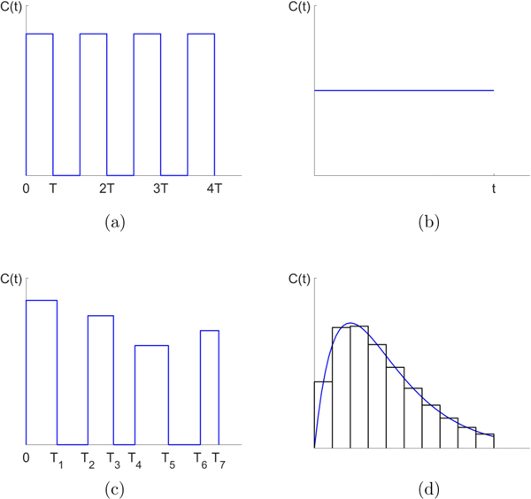
It is widely appreciated that the development of chemotherapeutic resistance is the primary reason for recurrence of cancer in patients undergoing treatment, and remains one of the primary challenges in the field of oncology [1–3]. As a tumor grows, and even as tumor cells spread throughout the system and metastasis ensues, standard prescheduled chemotherapeutic protocols such as maximum tolerated dose (MTD) and low-dose metronomic schedules (LDM) often show early success as the tumor regresses temporarily. Schematics for several kinds of chemotherapeutic schedules are shown in Fig. 1. A typical chemotherapeutic cycle might involve one strong dose every three weeks, or a dose for 5 consecutive days, followed by a 28 day rest period [4]. After months of fixed periodic cycles, the cancer often recurs and the tumor begins to regrow. Because of the genetic and cellular heterogeneity of a typical tumor [5], instead of killing all of the cancer cells and thereby eliminating the tumor, the chemotherapeutic regimen actually selects for a resistant phenotype [6–9]. The diversity of cells within a tumor effectively protects the tumor from single-line or prescheduled chemotherapeutic assaults by allowing for elimination of the chemo-sensitive population in order to accomplish the subsequent release of the chemo-resistant population. By reducing the relative fitness of the sensitive cells, chemotherapy acts as the primary mechanism of natural selection that selects specifically against rapidly dividing cells [10].
FIG. 1.
Schematic dose schedules. (a) Maximum tolerated dose (MTD) schedule. (b) Low dose metronomic (LDM) schedule. (c) Adaptive schedule. (d) General time-dependent schedule actuated by piecewise constant dose concentrations.
The characterization of a typical tumor as an adaptive landscape made up of competing cells of varying degrees of fitness, which determine growth rates of the various subpopulations, is a more accurate characterization of a tumor and suggests an ecological or evolutionary approach [11–20]. If one had access to time-resolved information [21] on the relative balance and growth rates of the subpopulations of cells making up the tumor, then one could use chemotherapy as a control device (actuator) to keep the subpopulations in balance, competing with each other indefinitely, without any one of the cancerous subpopulations dominating the landscape [6]. Chemotherapy would then be regarded more as a maintenance mechanism than a cure [22,23] and one would be imposing no more selection than is necessary, as has been advocated by Read et al. and others [24].
We introduce an evolutionary game theory model of chemotherapeutic resistance [1] along with a method of adaptive control to design advantageous chemotherapeutic schedules that are able to overcome, or at least manage, resistance. The mechanism of resistance that we model is based on the ecological notion of competitive release [8,11,25] of the resistant cell population when the sensitive cell population is reduced below a certain threshold. Above the threshold, the sensitive cells are able to outcompete (on average) the resistant cells due to the inherent cost of resistance [26], which tilts the fitness landscape of the system in favor of the sensitive cell population, allowing the tumor to grow. Under sufficient chemotherapeutic pressure, the sensitive cell population is reduced enough to allow the resistant population to begin to flourish and eventually regrow the tumor in a form that is much harder to treat. A quantitative understanding of this phenomenon is necessary in order to develop chemotherapeutic strategies (i.e., adaptive therapies) to combat it, a point of view adopted and developed in [3,13,14,16,22,27]. In this paper, we frame the problem as one in nonlinear dynamical systems theory and use trajectory transfer methods developed relatively recently in the orbital mechanics literature [28–32] to design chemotherapeutic schedules that have the potential to outperform more standard approaches [33].
The mathematical model we use is based on a three-component replicator dynamical system with a frequency-dependent fitness function based on a prisoner’s dilemma (PD) payoff matrix [34,35]. Cell interactions occur between three cell types that form our ecosystem: healthy cells (H), chemo-sensitive cells (S), and chemo-resistant cells (R). The healthy cell subpopulation can be thought of as non-neoplastic cells that have a lower fitness than the chemo-sensitive subpopulation. The independent variables represent relative frequencies in the total population, and the tumor alone would be made up of S + R cancer cell subpopulations. In a PD scenario, the healthy cells act as cooperators while the cancer cells act as defectors [36]. Unchecked, the defectors saturate the population as the average fitness decreases to a suboptimal outcome. The goal of chemotherapeutics in this framework is to coax the defectors to cooperate, leading to a higher fitness Nash equilibrium [34,35]. Growth rates are determined by cell fitness functionals which, in turn, depend on subpopulation sizes, i.e., they are frequency dependent. There is a time-dependent controller in our model which determines chemotherapeutic dose schedule and concentrations. Although the model system is nonlinear and the control parameter enters as a coefficient in most all of the terms of the three-component cubic nonlinear system (making classic control schemes [37] nonapplicable), we use nonlinear trajectory design techniques introduced and developed in an orbital mechanics context [28–32]. In that body of literature, time-dependent controllers are used to design orbit transfers in a Hamiltonian mechanics setting, piecing together partial orbits at different energy levels and switching energies at carefully chosen times, much like classic Hohmann transfers for satellite control [38]. While the replicator system we describe is not a Hamiltonian system in which orbits transfer from one energy level to another, the time-dependent chemotherapeutic parameter, C(t), can be used to design advantageous orbits in the replicator dynamics trilinear phase space in a similar manner where piecewise constant dose concentrations are used, Ci = const., for carefully chosen time intervals ti < t < ti+1 (i = 0,...,n) with switching times ti chosen in such a way as to produce a periodic (closed), continuous, piecewise differentiable orbit that stays trapped in a desirable region of the phase space. Orbits designed this way are shown to maintain a higher average level of fitness for the full population and avoid tumor recurrence. The existence of such orbits for appropriately chosen chemotherapeutic schedules in our model system suggests the possibility that similar orbits may also exist in a more complex tumor environment with carefully designed adaptive schedules [27,39]. The general technique of designing an orbit with a time-dependent controller should also work in other contexts such as microbial drug resistance [40] or pest management [8,41], although with perhaps different numbers of competing subpopulations and different payoff matrices that determine the fitness landscapes.
II. A THREE-COMPONENT REPLICATOR SYSTEM
The model we develop is based on a three-component replicator nonlinear dynamical system governing three competing subpopulations of cells: , where x1 represents the proportion of healthy cells (H), x2 represents the proportion of sensitive cells (S), and x3 represents the proportion of resistant cells (R), with x1 + x2 + x3 = 1. In this context, the model makes the well-mixed assumption on the cell population [34,35], i.e., no spatial dependence is modeled in order to highlight the method in as clean a setting as possible. For discussions and comparisons of well-mixed models vs those with spatial dependence, see [42]. The equations which describe the subpopulation interactions are
| (1) |
| (2) |
| (3) |
with fi representing the fitness of each of the subpopulations (i = 1,2,3) as their relative populations change, and representing the average fitness of the entire population. The exponential growth-decay rates of each of the subpopulations are then determined by , which dictates whether the subpopulation fitness is above or below the average population fitness, hence whether the subpopulation decays or grows.
The fitness of each of the three subpopulations is defined by the linear functionals
| (4) |
| (5) |
| (6) |
where are time-dependent selection parameters (that serve as our controllers) we use to shape the fitness landscape of the system. A is the payoff matrix associated with the cell-cell interactions, which we describe in Sec. III. The time dependence in our model enters through a chemo-concentration parameter C(t):
| (7) |
| (8) |
| (9) |
where w0 scales time (we typically take w0 = 1). Note that the chemotherapy parameter acts linearly on the sensitive cell population lowering its fitness, although the three populations are coupled nonlinearly through (1)–(3). The average population fitness is defined by the quadratic functional
| (10) |
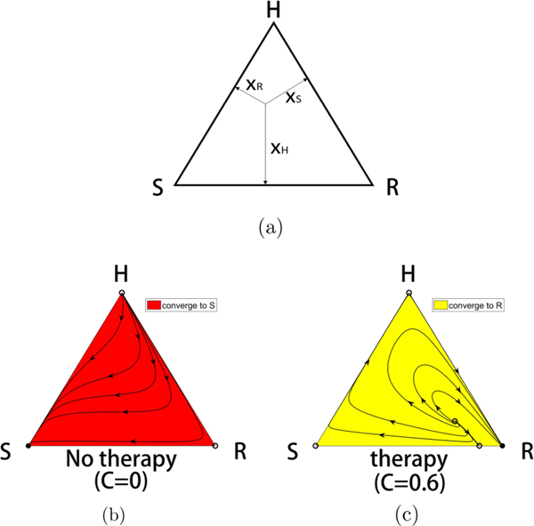
in the usual way. It is straightforward to see (for fixed values of the chemo-concentration parameter C) that the fixed points of the system (1)–(3) are of three basic types. (i) There are the three fixed points at each of the corners of the triangular phase space diagram shown in Fig. 2, when two of the subpopulation values are zero, and the third is saturated: . (ii) There are three possible fixed points on the triangle sides, which correspond to one of the subpopulation values equaling zero, with the other two having fitness values equal to the population average: . (iii) There is the balanced fitness state, when none of the subpopulation values is zero, but each of the subpopulation fitness values equals the population average: . Which of these fixed points lies on or inside the triangular phase space, and their stability properties, depend in detail on the parametric values, which we describe in Sec. IV.
FIG. 2.
The competitive release mechanism. (a) The three-component phase space associated with competing populations of (H,S,R) cells. (b) With no therapy, the S corner of the triangle is a globally attracting fixed point, while the H and R corners are unstable. All initial conditions lead to a saturated tumor. Filled circles are stable, unfilled circles are unstable. (c) For continuous chemotherapy above a threshold level, the R corner of the triangle is a globally attracting fixed point, while the H and S corners are unstable. All initial conditions (except those lying on the separatrix connecting the interior balanced fitness state to the S-R side) lead to a resistant tumor.
By using a prisoner’s dilemma payoff matrix (see Sec. III) we ensure (i) Gompertzian growth of the cancer cells [43], (ii) a reduction in overall fitness of the population as the tumor grows, and (iii) a fitness cost associated with resistance. We first study the details of the nonlinear dynamics associated with Eqs. (1)–(3) for constant values of the chemotherapy parameter to demonstrate the mechanism of competitive release for threshold values . Then we investigate piecewise constant time-dependent functions C(t) to show how to avoid the evolution of resistance of the tumor. Figure 1 shows several examples of the chemotherapeutic schedules we consider. These include maximum tolerated dose (MTD) schedules [Fig. 1(a)], low-dose metronomic schedules (LDM) [Fig. 1(b)], adaptive schedules [Fig. 1(c)], and more general time-dependent schedules [Fig. 1(d)] which we break up into piecewise constant doses as done when forming the Riemann sum approximation to an area under a curve. In all cases, we compare outcomes of the different schedules holding the total dosage, D, fixed over time period τ,
| (11) |
III. THE PRISONER’S DILEMMA AS A CANCER MODEL
We first describe the standard version of the PD payoff matrix [34] in a 2 × 2 setting to make clear why the PD evolutionary game gives rise to a Gompertzian (i.e., “S-shaped”) growth curve when two subpopulations compete. To be specific, we first describe what happens when healthy cells compete with cancer cells using the 2 × 2 payoff matrix
| (12) |
with c > a > d > b. The first row and column correspond to the payoffs associated with the cooperator (C) in the PD evolutionary game, and the second row and column correspond to the payoffs associated with the defector (D). In the simplest tumor growth paradigm in which a population of healthy cells competes with a population of cancer cells, the healthy cells are the cooperators, while the cancer cells are the defectors. In any mixed population the fitness functions, , associated with the two subpopulations are
| (13) |
which in component form yields
| (14) |
| (15) |
while the average fitness of the total population is given by the quadratic form
| (16) |
Note that the average fitness of the healthy state (xC, xD) = (1,0) is given by , while that of the cancerous state (xC, xD) = (0,1) is given by 1, which minimizes the average fitness. Tumor growth is then modeled as a 2 × 2 evolutionary game governed by the replicator dynamical system:
| (17) |
| (18) |
It is straightforward to show
with fixed points at. . From this, we can conclude that for any initial condition containing at least one cancer cell, , we have
.
Condition (i) guarantees that the cancer cell population will saturate, while condition (ii) guarantees that the saturated state is suboptimal, since. For these two reasons, the prisoner’s dilemma evolutionary game serves as a simple model for tumor growth both in finite population models as well as replicator system (infinite population) models [18–20,44].
For our purposes, we now generalize to a three-component system where the fitness functions (4)–(6) are defined via a payoff matrix A which is a 3 × 3 matrix defining the evolutionary game played by the cell population. For this, we take every 2 × 2 submatrix to be a PD game, i.e., we take A to be the 3 × 3 PD matrix
| (19) |
with the PD inequalities [34]:
| (20) |
| (21) |
| (22) |
The numerical values in (19) are chosen for convenience and satisfy the constraints (20)–(22). In each cell-cell interaction, the healthy cells x1 (healthy H) are cooperators, and the two species of cancer cells, x2 (sensitive S) and x3 (resistant R), are the defectors. In any interaction between a chemo-sensitive cell (S) and a chemo-resistant cell (R), the sensitive cell is the defector, while the resistant cell is the cooperator. The payoff matrix (19) guarantees that, for any interaction between two cells, the system retains features (i) and (ii) detailed previously (i.e., tumor growth leading to suboptimal fitness). In addition, the payoff matrix also imposes a cost to resistance if we add the extra constraint d > g which guarantees
| (23) |
It is worth pointing out that shaping the fitness landscape by adjusting the selection parameters (w1,w2,w3) is equivalent to choosing
| (24) |
where
To see this, use the fact that in the fitness equations (4)–(6).
IV. RESULTS
A. Continuous therapy
For the purposes of understanding how to implement time-dependent therapies in our model, we first describe the phase space dynamics for constant values , so total dose delivered over time period t is D = Ct. Figure 2 shows the mechanism of chemotherapeutic resistance via competitive release determined by the system (1)–(3) (for constant C) as depicted in the triangular phase space diagram shown in Fig. 2(a). With no therapy [Fig. 2(b), C = 0], the sensitive corner S is globally attracting, while the H and R corners are unstable. When the continuous therapy parameter C = 0.6 [Fig. 2(c)], the resistant corner is globally attracting, while the H and S corners are unstable. Filled corners are stable, unfilled corners are unstable. This is the basic mechanism of competitive release induced by sufficiently strong chemotherapeutic dose [6].
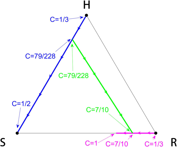
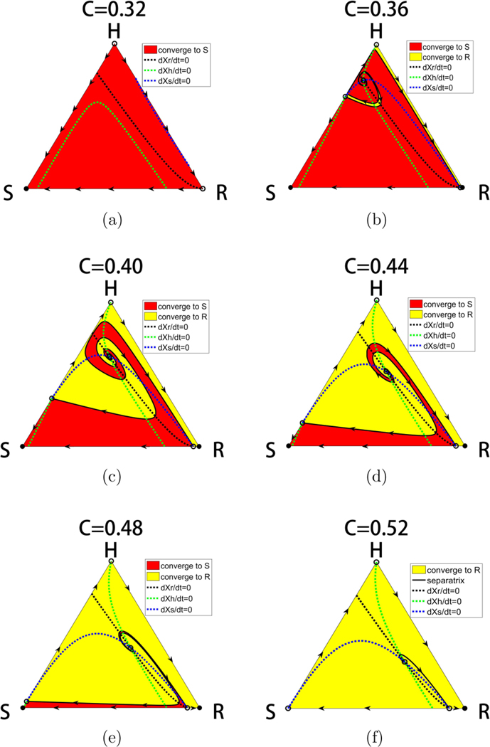
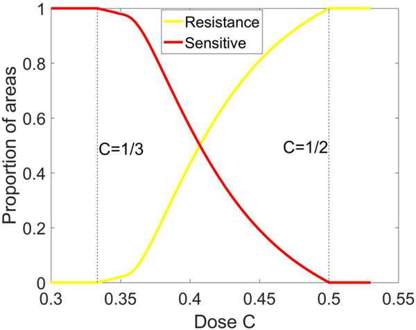
Intermediate values of C reveal a much more complex picture. We show in Fig. 3 the location of the fixed points as a function of C. For values , the balanced fixed point state is an interior fixed point, which forms the central spiral associated with the basin boundaries between the asymptotically stable S corner and R corner, shown in Fig. 4. Also shown in the figure are the nullclines defined by the curves . Opposite sides of each of the nullclines mark a change in whether the particular subpopulation decays or grows. The mixed population state exists for values 1/3 < C < 1/2 where the basin of attraction sizes (areas), shown in Fig. 5, change sensitively (as C varies), one at the expense of the other, in an intertwined spiral structure centered at the balanced fixed point state. The steep transition curves between the two states occurring for small changes in the chemo-concentration parameter highlights the sensitivity of the system to chemotherapeutic dosing levels. Also worth highlighting in Figs. 4(b) and 4(c) is the sensitivity to resistant mutations of the final asymptotic state of the system, even if no preexisting mutations exist in the population. As the tumor grows, assuming no preexisting resistant mutations, the dynamics would traverse down the left side of the triangle from the H corner to the S corner. As it does, the very thin passageway [on the H-S side of the triangle in Figs. 4(b) and 4(c)] associated with the basin of attraction of the resistant corner indicates that one single resistant mutation would push the trajectory off the side into the basin of attraction associated with the R corner instead of converging to the S corner.
FIG. 3.
Fixed point locations. Tracking the location of the fixed points as a function of chemo-concentration parameter C. The fractional values indicate that the values are analytically obtained.
FIG. 4.
Basins of attraction and nullclines. Panel showing the separatrices and nullclines through the balanced fitness interior fixed point that determines the basin boundaries of attraction of the S state and the R states. The interior fixed point is the one in which each of the subpopulation fitness levels exactly matches the average fitness of the entire population. Filled circles are stable, unfilled circles are unstable.
FIG. 5.
Basin of attraction areas. Areas of basin of attraction of S fixed point and R fixed point as a function of chemo-concentration C.
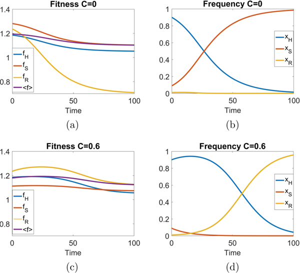
The fitness landscapes are shown in Fig. 6 both for C = 0 and for C = 0.6. With no therapy, the fitness curves are monotonically decreasing functions as the sensitive population saturates the tumor in a sigmoidal shaped [18,43] growth curve. With continuous therapy above threshold, the fitness curves initially increase (i.e., tumor regression), but eventually decrease monotonically as the tumor relapses. The healthy cell population initially increases, but eventually the resistant population saturates the tumor.
FIG. 6.
Fitness landscapes as a function of time. With no therapy (C = 0), the fitness curves are continuously decreasing functions as the tumor saturates with the sensitive cell population in a sigmoidal shaped growth curve. With continuous therapy (C = 0.6), the fitnesses initially increase indicating tumor regression, but eventually decrease. The healthy subpopulation initially increases before the resistant population eventually saturates the tumor. Initial condition (0.9,0.09,0.01) with w0 = 0.1
B. Time-dependent therapy
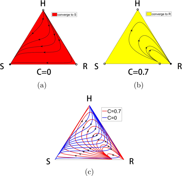
Figure 7 shows the key idea behind the method we use to design trajectories for Eqs. (1)–(3) for time-dependent chemotherapeutic schedules C(t). With no chemotherapy, C = 0, since the sensitive corner S is a globally asymptotically attracting fixed point whose basin of attraction is the full region, all trajectories that start inside the triangle eventually get trapped in the left S corner. By contrast, with chemotherapeutic levels at C = 0.7, competitive release acts to create a basin of attraction for the right resistant corner R for all initial conditions inside the triangle. Using these families of solution trajectories, we overlay the solution curves in Fig. 7(c) to show the underlying curvilinear grid that spans the full trilinear phase plane. By switching between the two values C = 0 and C = 0.7 at times when two curves intersect, it is possible to transition from a trajectory associated with the C = 0 family to one associated with the C = 0.7 family. This creates multiple possibilities for designing complex orbits using piecewise constant values of C, with switching at appropriately chosen times.
FIG. 7.
Dynamical trajectories for constant C. (a) With no chemotherapy (C = 0), the sensitive corner S is a globally attracting fixed point. All initial conditions inside the triangle move to S along the sample trajectories shown. (b) Above the chemotherapy threshold C > 0.5, all initial conditions inside the triangle move to the resistant corner R. Shown are sample trajectories for C = 0.7. (c) Overlay of the solution trajectories for C = 0 and C = 0.7 create a curvilinear grid throughout the triangle. By switching between these two values of C, we construct a global trajectory made up of segments of the two families of trajectories.
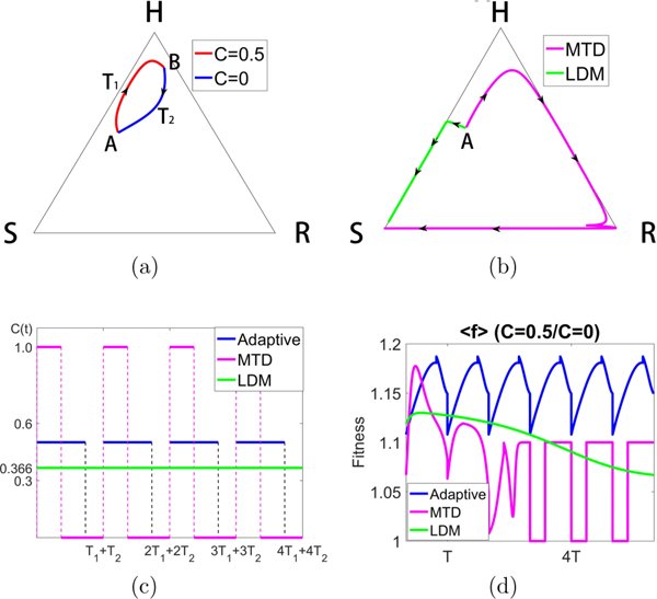
One such trajectory is shown in Fig. 8(a), achieved by switching between the two values C = 0 and C = 0.5. The trajectory starts at point A [(H, S, R) = (0.5, 0.4, 0.1)] using a trajectory with C = 0.5. When the trajectory reaches point B, the chemotherapy is switched off, C = 0, and the system then travels back down to point A in a closed loop. With switching times labeled T1 and T2 (which are computed by monitoring the relative balances of the three subpopulations), this closed orbit can be maintained indefinitely. By contrast, Fig. 8(b) shows the corresponding MTD and LDM trajectories with the same initial condition (point A) using the same total dosages over the same time periods. The MTD trajectory eventually gets trapped in the left S corner, as does the LDM trajectory. Figure 8(c) shows the schedules for all three cases. In all cases, we first design the adaptive schedule, then we create the MTD and LDM schedules using the same total dosage D. Neither the MTD nor the LDM standard chemo-schedules are able to prevent the system from saturating with a full grown tumor, whereas the adaptive schedule keeps the system trapped indefinitely near the top H corner of the system. Figure 8(d) shows the average fitness of the system for the MTD, LDM, and adaptive schedules. It is clear that the adaptive schedule is able to maintain a higher average fitness throughout the full course of chemotherapy.
FIG. 8.
Constructing a closed loop trajectory using C = 0 and C = 0.5, with Cavg = 0.366. (a) By using segments of a trajectory for C = 0 and C = 0.5, switching values at points A and B, we construct a closed periodic orbit. (b) Using the same total dose, we show the MTD and LDM trajectories starting from point A. Both eventually move to the S corner, although initially the MTD trajectory moves toward the H corner (tumor regression) before recurrance. (c) The MTD, LDM, and adaptive schedules are depicted. (d) We plot the average fitness for the three different chemo-schedules. The adaptive schedule is able to maintain a higher average fitness throughout.
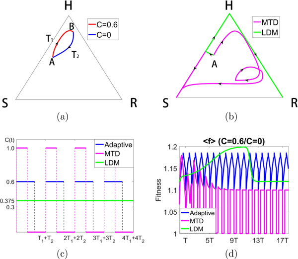
Figure 9 shows the sensitivity of the system to the chemo-concentration levels chosen. Here we switch between C = 0 and C = 0.6 (higher average dose than in Fig. 8) to construct the closed loop [Fig. 9(a)], which looks very similar to that in Fig. 8. But notice that for these values the LDM schedule creates an orbit that saturates at the R corner, whereas the MTD schedule saturates at the S corner. The actual schedules are shown in Fig. 9(c). Figure 9(d) compares the average population fitness of the three schedules, showing that the adaptive schedule maintains a higher average throughout. Notice that LDM initially achieves a higher average fitness before tumor regression occurs.
FIG. 9.
Constructing a closed loop trajectory using C = 0 and C = 0.6, with Cavg = 0.375. (a) By using segments of a trajectory for C = 0 and C = 0.6, switching values at points A and B, we construct a closed periodic orbit. (b) Using the same total dose, we show the MTD and LDM trajectories starting from point A. The MTD trajectory eventually moves to the S corner, while the LDM trajectory moves to the R corner. Both trajectories initially move toward the H corner (tumor regression) before recurrence. (c) The MTD, LDM, and adaptive schedules are depicted. (d) We plot the average fitness for the three different chemo-schedules. The adaptive schedule is able to maintain a higher average fitness throughout, although LDM initially achieves higher average fitness before declining.
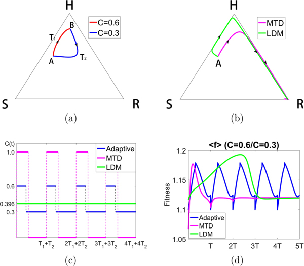
In Fig. 10 we show the result of toggling between values C = 0.3 and C = 0.6 to maintain the periodic loop [Fig. 10(a)]. For this case, both the MTD and LDM schedules send the trajectory to the R corner [Fig. 10(b)]. Figure 10(d) shows the initial benefit of the MTD and LDM schedules in terms of higher initial average fitness, but eventually the adaptive schedule shows its superiority over both.
FIG. 10.
Constructing a closed loop trajectory using C = 0.3 and C = 0.6, with Cavg = 0.396. (a) By using segments of a trajectory for C = 0.3 and C = 0.6, switching values at points A and B, we construct a closed periodic orbit. (b) Using the same total dose, we show the MTD and LDM trajectories starting from point A. Both trajectories move toward the R corner after initially moving toward H. (c) The MTD, LDM, and adaptive schedules are depicted. (d) We plot the average fitness for the three different chemo-schedules. The adaptive schedule is able to maintain a higher average fitness throughout. Both MTD and LDM initially show higher average fitness before declining.
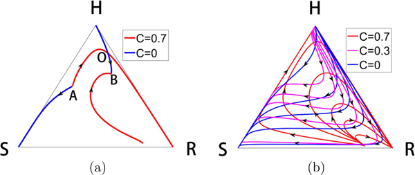
Figure 11(a) shows that we can actually design an orbit that starts at an arbitrary point A inside the triangle, and send it to an arbitrary point B. We accomplish this by constructing the incoming and outgoing orbits from point A for two different C values, and those associated with point B for those same two C values, showing that they must intersect at some point which we label O. By sending the orbit out from point A to point O, then switching values of C at point O until we arrive at point B, we complete the transfer. One can immediately see the potential richness in the possible design of different orbits one can construct by switching values of C among two, three, or more values, at appropriately chosen times. Figure 11(b) shows the richness of the curvilinear grid that can be created with three values of C = 0,0.3,0.7 and the multitude of possible paths from one point to another inside the triangle if one allows for switching among the three values shown.
FIG. 11.
Constructing orbit transfers. (a) We take two arbitrary points labeled A and B and construct the incoming and outgoing solution trajectories from each, using two values C = 0 and C = 0.7. There must be a crossing point, which we label point O. The two segments AO followed by OB is the two-switch trajectory that takes us from A to B. (b) Shown is the curvilinear grid constructed by families of solution curves for the three values C = 0, C = 0.3, C = 0.7. Any point of intersection can be used as a starting point and an ending point to construct a three-switch orbit.
C. Robustness
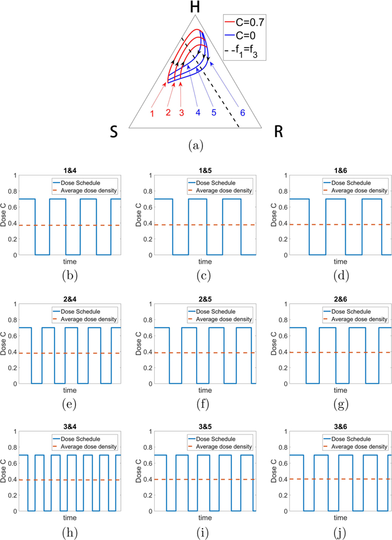
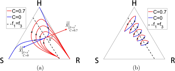
To be clinically actionable, at the very least it would be important that the method not be sensitive to specific initial conditions and parameter values. We describe several remarkably robust features of the strategy in this section. We show in Fig. 12(a) an example of a continuous family of closed orbits that are easily achievable by using a bang-bang strategy, with blue orbits (no therapy) and red orbits (C = 0.7) forming a continuous family of closed and nearly closed loops. The associated dose schedules are shown in Figs. 12(b)–12(j), with average doses all very close to 0.4. Because of the continual interlacing of these orbits, and the robustness of their associated schedules, it is clear there is nothing particularly special about any of the values shown, or the average dose; any of the orbits and schedules would work. Interestingly, Fig. 13 shows that the entire region on the right side of the triangle centered on the dashed curve can be populated by continuous families of closed orbits, each centered at any point on the line. Figure 13(a) depicts the defining feature of the line which requires that two orbits with different C values have a point of tangency lying on it. A necessary and sufficient condition for this is f1 = f3, which defines a line; a condition obtained by requiring that tangent vectors associated with two different values of C point in opposite directions, as shown in Fig. 13(a). Figure 13(b) shows examples of closed orbits obtained at five representative points on the dashed line.
FIG. 12.
Robust family of nested orbits. (a) One example of a (continuous) family of nested closed orbits using bang-bang strategy toggling between C = 0 and C = 0.7, all with similar total dose (C ∼ 0.4). A closed loop can be made arbitrarily small around a center point described in Fig. 13. Schedules associated with (b) orbits 1 and 4; (c) orbits 1 and 5; (d) orbits 1 and 6; (e) orbits 2 and 4; (f) orbits 2 and 5; (g) orbits 2 and 6; (h) orbits 3 and 4; (i) orbits 3 and 5; (j) orbits 3 and 6.
FIG. 13.
All closed orbit families are centered on dashed line defined by f1 = f3. (a) As a family of closed orbits enclose smaller and smaller loops, they intersect at a point of tangency. The point of tangency must lie on the dashed line. (b) Examples of several closed loop orbits centered at different points down the line.
V. DISCUSSION
The model shows that if the chemo-dose exceeds a threshold value of C > 0.5, the tumor may regress for a period of time, but eventually regrows to form a resistant tumor [Fig. 2(c)] as long as there is at least one resistant cell in the population (i.e., a preexisting resistant mutation). This process of competitive release is very robust and occurs for all initial distributions of the three subpopulations. For chemo-doses that are not as large, the results are much more sensitive to small changes in C since the phase space diagram generally has two basins of attraction, one associated with a saturated sensitive state and the other with a saturated resistant state, and these basins of attraction are spirally intertwined. Small differences in the balances among the three types of cells comprising our model, and a single resistant mutation, can determine whether the long-time dynamics converges to the S state or the R state. The relative areas of the basins of attraction also sharply change with small changes in chemo-dose values between 1/3 < C < 1/2, reflecting the sensitivity in choosing the optimal chemo-dose levels. There is no constant value of C for which the system converges to the H state, as this state is always unstable.
By contrast, for a time-dependent chemotherapy parameter C(t), one can design a rich, robust, and potentially endless array of trajectories (i.e., tumor responses) that remain in desirable regions of the triangular phase space indefinitely, depending on how many time switches and different dose levels one is willing to accept. One can, in principle, steer the system trajectory along any path (in the model). Identifying a given trajectory in our model as well as the chemo-therapeutic schedule that produces it is fairly straightforward and amounts to superposing the response curves associated with different constant therapies, and piecing together a global trajectory made up of sections generated from each of the constant therapy curves. Of course, in a clinical setting this procedure will be much more complex, but it suggests the possibility of using actual chemo-therapeutic responses with different chemo-schedules used on different patients as a design template to combine in new ways to predict possible responses to various time-dependent switching strategies. By using one dosing schedule to create a time-limited response, then a different dosing schedule to create a different (time-limited) response, one could think of piecing together finite-time limited responses to create new outcomes, superior to what would have been achieved by sticking to one single chemo-schedule.
One of the challenges of testing and designing new schedules via clinical trials is that short term gain in average fitness with LDM or MTD does not always result in more long-term increased averaged fitness levels, i.e., recurrence sets in if the schedule does not completely eradicate the tumor. This is clearly shown in our simulations. The possibility of designing complex orbits with various potentially advantageous features is virtually endless if one allows for enough switches among many different levels of the chemo-concentration parameter C. In this paper, we have focused on comparisons of average fitness levels to evaluate the quality of the schedule. One could, of course, imagine designing orbits that maximize a (time-averaged) population fitness while minimizing total dose, or perhaps delay recurrence as long as possible while avoiding regions of the phase space (i.e., relative balances of the subpopulation levels) where the total tumor burden becomes unsustainable. The fact that closed loop trajectories can be designed in our model three-component replicator system by chemo-scheduling alone suggests the possibility that similar orbits could potentially be created in an actual tumor environment, microbial environment, or pest management setting with the right actuation (chemo-schedule, antibiotic regimen, or pest control schedule), where fixation of the sensitive population or fixation of the resistant population are both avoided indefinitely as the balance is managed with proper adaptive therapy. This, of course, all hinges on our ability to carefully and frequently monitor the tumor environment [21]. Clinical trials that make use of adaptive scheduling ideas are currently being carried out at the Moffitt Cancer Center, and results show great promise [39]. More possibilities exist with the use of combination multidrug therapies [13,40,45] or immunotherapies [46], but these are outside the scope of our model, which focuses only on the use of dosing schedules to shape the fitness landscape of a tumor to steer its evolutionary response.
ACKNOWLEDGMENTS
We gratefully acknowledge partial support from the Breast Cancer Research Foundation (BCRF) and the Jayne Koskinas & Ted Giovanis Foundation (JKTG) for Health and Policy. We thank S. Anderson, D. Basanta, J. Brown, H. Enderling, R. Gatenby, and J. West at the Moffitt Cancer Research Center for helpful conversations regarding this and related work.
Contributor Information
P. K. Newton, Department of Aerospace & Mechanical Engineering, Department of Mathematics, and Norris Comprehensive Cancer Center, University of Southern California, Los Angeles, California 90089-1191, USA.
Y. Ma, Department of Physics & Astronomy, University of Southern California, Los Angeles, California 90089-1191, USA.
References
- [1].Komarova N. and Wodarz D, Proc. Natl. Acad. Sci. USA 102, 9714 (2005). [DOI] [PMC free article] [PubMed] [Google Scholar]
- [2].Aktipis C, Kwan V, Johnson K, Neuberg S, and Maley C, PloS One 6, e26100 (2011). [DOI] [PMC free article] [PubMed] [Google Scholar]
- [3].Bozic I. and Nowak M, Annu. Rev. Cancer Bio. 1, 203 (2017). [Google Scholar]
- [4].Perry M, The Chemotherapy Source Book (Lippincott Williams & Wilkins, Philadelphia, 2008). [Google Scholar]
- [5].Venkatesan S. and Swanton C, in American Society of Clinical Oncology Educational Book, Vol. 36 (ASCO, Alexandria, VA, 2016), p. e141. [DOI] [PubMed] [Google Scholar]
- [6].Seton-Rogers S, Nat. Rev. Cancer 16, 199 (2016). [DOI] [PubMed] [Google Scholar]
- [7].Gatenby R. and Brown J, Cold Spring Harb. Perspect. Med. 8, a033415 (2018). [DOI] [PMC free article] [PubMed] [Google Scholar] [Retracted]
- [8].Gould F, Am. Sci. 79, 496 (1991). [Google Scholar]
- [9].Connell JH, Ecology 42, 710 (1961). [Google Scholar]
- [10].Lewontin R, Annu. Rev. Ecol. Syst. 1, 1 (1970). [Google Scholar]
- [11].Merlo LM, Pepper JW, Reid BJ, and Maley CC, Nat. Rev. Cancer 6, 924 (2006). [DOI] [PubMed] [Google Scholar]
- [12].Attolini CS-O and Michor F, Ann. N.Y. Acad. Sci. 1168, 23 (2009). [DOI] [PubMed] [Google Scholar]
- [13].Basanta D, Gatenby R, and Anderson A, Mol. Pharmaceutics 9, 914 (2012). [DOI] [PMC free article] [PubMed] [Google Scholar]
- [14].Basanta D. and Anderson A, Interface Focus 3, 20130020 (2013). [DOI] [PMC free article] [PubMed] [Google Scholar]
- [15].Enriquez-Navas PM, Kam Y, Das T, Hassan S, Silva A, Foroutan P, Ruiz E, Martinez G, Minton S, Gillies RJ et al. , Sci. Transl. Med. 8, 327ra24 (2016). [DOI] [PMC free article] [PubMed] [Google Scholar]
- [16].Silva A. and Gatenby R, Biol. Direct 5, 25 (2010). [DOI] [PMC free article] [PubMed] [Google Scholar]
- [17].Beckman R, Schemmarm G, and Yeang C, Proc. Natl. Acad. Sci. USA 109, 14586 (2012). [DOI] [PMC free article] [PubMed] [Google Scholar]
- [18].West J, Hasnain Z, Macklin P, and Newton PK, SIAM Rev. 58, 716 (2016). [DOI] [PMC free article] [PubMed] [Google Scholar]
- [19].West J. and Newton PK, Cancer Res. 77, 1 (2017). [DOI] [PMC free article] [PubMed] [Google Scholar]
- [20].West J, Hasnain Z, Mason J, and Newton PK, Convergent Sci. Phys. Oncol. 2, 035002 (2016). [DOI] [PMC free article] [PubMed] [Google Scholar]
- [21].Fisher A, Vazquez-Garcia I, and Mustonen V, Proc. Natl. Acad. Sci. USA 112, 1007 (2015). [DOI] [PMC free article] [PubMed] [Google Scholar]
- [22].Gatenby R, Nature (London) 459, 508 (2009). [DOI] [PubMed] [Google Scholar]
- [23].Jamsen G, Gatenby R, and Aktipis C, Proc. Natl. Acad. Sci. USA 112, 937 (2015). [DOI] [PMC free article] [PubMed] [Google Scholar]
- [24].Read A, Day T, and Huijben S, Proc. Natl. Acad. Sci. USA 108, 10871 (2011). [DOI] [PMC free article] [PubMed] [Google Scholar]
- [25].Segre H, DeMalach N, Henkin Z, and Kadmon R, PloS One 11, e0160798 (2016). [DOI] [PMC free article] [PubMed] [Google Scholar]
- [26].Andersson D. and Levin B, Curr. Opin. Microbiol. 2, 489 (1999). [DOI] [PubMed] [Google Scholar]
- [27].Gatenby R, Silva A, Gillies R, and Frieden B, Cancer Res. 69, 4894 (2009). [DOI] [PMC free article] [PubMed] [Google Scholar]
- [28].Koon WS, Lo MW, Marsden JE, and Ross SD, Chaos 10, 427 (2000). [DOI] [PubMed] [Google Scholar]
- [29].Gomez G, Koon W, Lo M, Marsden J, and Ross S, Nonlinearity 17, 1571 (2004). [Google Scholar]
- [30].Grover P. and Ross S, J. Guid. Control Dyn. 32, 436 (2009). [Google Scholar]
- [31].Ross S. and Scheeres D, SIAM J. Appl. Dyn. Sys. 6, 576 (2007). [Google Scholar]
- [32].Radu S, Koon W, Lo M, Marsden J, Ross S, and Wilson R, Automatica 38, 571 (2002). [Google Scholar]
- [33].Norton L. and Simon R, Cancer Treat. Rep. 61, 1307 (1977). [PubMed] [Google Scholar]
- [34].Nowak MA, Evolutionary Dynamics (Harvard University Press, Cambridge, MA, 2006). [Google Scholar]
- [35].Hofbauer J. and Sigmund K, Evolutionary Games and Population Dynamics (Cambridge University Press, Cambridge, UK, 1998). [Google Scholar]
- [36].Axelrod R, Axelrod DE, and Pienta KJ, Proc. Natl. Acad. Sci. USA 103, 13474 (2006). [DOI] [PMC free article] [PubMed] [Google Scholar]
- [37].Bratton K, Ledzewicz U, and Schattler H, Biomath. Commun. 1, 1 (2014). [Google Scholar]
- [38].Prussing J. and Conway B, Orbital Mechanics, 2nd ed. (Oxford University Press, Oxford, 2013). [Google Scholar]
- [39].Zhang J, Cunningham J, Brown J, and Gatenby R, Nat. Commun. 8, 1816 (2017). [DOI] [PMC free article] [PubMed] [Google Scholar]
- [40].Nichol D, Jeavons P, Fletcher AG, Bonomo RA, Maini PK, Paul JL, Gatenby RA, Anderson ARA, and Scott JG, PLoS Comput. Biol. 11, e1004493 (2015). [DOI] [PMC free article] [PubMed] [Google Scholar]
- [41].Brown J. and Stankova K, Curr. Opin. Insect Sci. 21, 26 (2017). [DOI] [PubMed] [Google Scholar]
- [42].You L, Brown J, Thuijsman F, Cunningham J, Gatenby R, Zhang J, and Stankova K, J. Theor. Biol. 435, 78 (2017). [DOI] [PubMed] [Google Scholar]
- [43].Norton L, Cancer Res. 48, 7067 (1988). [PubMed] [Google Scholar]
- [44].Traulsen A, Claussen JC, and Hauert C, Phys. Rev. Lett. 95, 238701 (2005). [DOI] [PubMed] [Google Scholar]
- [45].Yoon N, Vander Velde R, Marusyk A, and Scott JG, Bull. Math. Bio. 80, 1776 (2018). [DOI] [PubMed] [Google Scholar]
- [46].Restifo NP, Dudley ME, and Rosenberg SA, Nat. Rev. Immunol. 12, 269 (2012). [DOI] [PMC free article] [PubMed] [Google Scholar]


