FASTQINS and ANUBIS: two bioinformatic tools to explore facts and artifacts in transposon sequencing and essentiality studies

Abstract

Transposon sequencing is commonly applied for identifying the minimal set of genes required for cellular life; a major challenge in fields such as evolutionary or synthetic biology. However, the scientific community has no standards at the level of processing, treatment, curation and analysis of this kind data. In addition, we lack knowledge about artifactual signals and the requirements a dataset has to satisfy to allow accurate prediction. Here, we have developed FASTQINS, a pipeline for the detection of transposon insertions, and ANUBIS, a library of functions to evaluate and correct deviating factors known and uncharacterized until now. ANUBIS implements previously defined essentiality estimate models in addition to new approaches with advantages like not requiring a training set of genes to predict general essentiality. To highlight the applicability of these tools, and provide a set of recommendations on how to analyze transposon sequencing data, we performed a comprehensive study on artifacts corrections and essentiality estimation at a 1.5-bp resolution, in the genome-reduced bacterium Mycoplasma pneumoniae. We envision FASTQINS and ANUBIS to aid in the analysis of Tn-seq procedures and lead to the development of accurate genome essentiality estimates to guide applications such as designing live vaccines or growth optimization.

INTRODUCTION

Synthetic biology aims to rationally design living systems for practical applications. Ideally, this requires a comprehensive understanding of the organism and a reduction of its genome by removing dispensable genes to create a so-called ‘chassis’ (1). Transposon mutagenesis is one of the most informative methods for identifying non-essential genes and understanding what is the minimal set of genes required to sustain life. This technique relies on the random disruption of genes to discriminate between those genes that do not accept insertions and thus are required to sustain life (‘essential’; E), those that when inactivated decrease the fitness of the organism (‘fitness’; F), and those which are dispensable under the study conditions (‘non-essential’; NE) (2). Disruption of genes by transposable elements is commonly driven by transposases (3). Transposases are enzymes able to randomly insert genetic material into genome regions delimited by inverted repeats (IR) and they can be classified in two types depending on insertion site preferences: Tc1/mariner transposases, that are able to disrupt TA dinucleotide sites, and Tn-5 based transposases, which are assumed to insert without sequence composition restrictions (4). After transforming the cells, the number of insertion sites in the population, or ‘coverage’, should ideally reach the maximum (i.e. every possible genome position disrupted at least once). Then, mutant cells are selected for by subsequent growth and serial passages. After several rounds of division, cells in which an E gene has been disrupted will disappear from the population and only NE genes will have insertions. Remarkably, essentiality in an organism may vary between different genetic and/or environmental conditions like during infection (5). Transposon insertion sites are commonly identified by ultra-deep sequencing in a technique known as Transposon sequencing (Tn-seq) (6–8). Unfortunately, analysis of Tn-seq data to determine gene essentiality is not straightforward and both biological and technical factors can result in errors. In addition, essentiality is not Boolean (E or NE); there is also a third set of genes called fitness genes (F), in which the probability to find insertions depends on the capability of mutants carrying these mutations to compete with the culture population. Hence, F genes can be defined as NE or E depending on the rounds of passaging selection and experimental conditions (7). In E genes, it is common to find insertions in the N- and C-terminal regions as these are not expected to disrupt the functional core of the encoded protein (9–12). Presence of NE domains and high abundance and long protein half-lives are also factors to consider (7). For example, cells with an insertion in an E gene that encodes a protein with a long half-life will still survive until the corresponding protein is not depleted through dilution by cell division. Similarly, the gene of an essential metabolic enzyme could have insertions until the metabolite produced by the enzyme runs out. Finally, due to the high sensitivity of deep sequencing, it cannot be discarded that transposon insertions occurring in E regions (not viable) could still be detected if dead cells with those insertions remain in the sample.

At the technical level, increased read counts for an insertion position can be found because of PCR duplicates that are produced during the transposon sequence enrichment step (13) (see Supplementary Figure S1). Despite available software being able to count these duplicates as one (14,15), the effect of removing the duplicates on essentiality assignment is still unclear. Also, in Tn-seq the exact insertion position can be miss-mapped due to a high error rate when sequencing specific regions such as homopolymers (16). Miss-mapped insertions can also arise due to chimeric sequences, which can be generated when combining chromosomal DNA with the inserted sequence, and that by chance, may match another genomic locus (17). Furthermore, there can be issues regarding the transposon insertion itself because different transposases prefer different nucleotide compositions. For example, the Tc1/mariner transposase only disrupts TA dinucleotides sites and as such, it is necessary to correct for the GC content (18). Even the Tn5-based transposases, which presumably do not present this bias (19), have been reported to favor AT-rich regions (7). Some transposases also produce staggered cuts that result in target site duplications (TSD) (20,21). The impact of these factors on the analyses and interpretation of Tn-seq data has not yet been addressed.

Finally, when running Tn-seq experiments it is also important to consider how essentiality is estimated. Multiple approaches have been proposed and include different metrics, normalizations (22,23) and methods based on different statistical models (9,24–26). A complete Tn-seq analysis requires multiple parameters as well as the use of a training set of genes or ‘gold set’ that can introduce additional biases depending on the assumptions taken. For example, to define a NE gold set some models took genes not conserved in closely-related species (7) while others use non-coding regions (25). This problem is especially important in organisms with little or no knowledge on their basic biology. In general, software tools to extract insertion profiles and posterior analyses of Tn-seq procedures are focused on Tc1/mariner-based protocols (27–29) and are not really applicable for Tn5-based Tn-seq as they only account for TA site disruption. Although a variety of methods have been proposed, there is still no in-depth study aimed at understanding how the combination of data treatments with different assumptions and approaches impacts the extraction of essentiality information.

To solve the above issues in an unbiased manner, we have developed two software packages: (i) a pipeline for the detection of transposon insertions called FASTQINS and (ii) a framework for the ANalysis of UnBiased InSertions, or ANUBIS (Figure 1A). Together, these packages take into account the aforementioned issues that are ignored in currently available bioinformatic solutions (Figure 1B), and create a benchmark to facilitate comparison, analysis and assessment of genome essentiality. To test the methodology we generated a Tn-seq dataset by transforming the genome-reduced bacterium Mycoplasma pneumoniae with the mini-transposon pMTnCat_BDPr, which encodes the Tn5-like transposase Tn4001 (Figure 1C). This microorganism has a genome of ∼860 kb, 40% GC-content, 689 protein-coding genes and is an excellent systems and synthetic biology model organism (30,31). In addition, M. pneumoniae presents unprecedented high transposon transformation efficiency rates that ensure a high initial insertional coverage along the genome (1 insertion every ∼3 bp in this study; 1 insertion every ∼4 bp in a previous study (7)), preserved when only considering coding regions (two insertions every ∼7 bp). Using this model, we analyzed multiple rounds of passage selection and the associated essentiality estimates (Figure 1D). Using ANUBIS, we then compared different essentiality landscapes by passage, processing steps, and model estimates (Figure 1E).

Figure 1.

Graphical abstract. (A) Proposed workflow using FASTQINS to process raw sequencing files into insertion profiles and ANUBIS to explore essentiality-related problems and provide estimates. (B) Graphical representation of the different issues that are not considered in previous essentiality studies. Target site duplications can double the signal of a transposition event (the transposon in blue is flanked by two different chromosome positions that are at a fixed distance equal to the duplication size). Reads derived from the PCR process can artifactually increase the signal of an insertion point (symbolized as triangles). GC content biases can occur when a transposase shows preference for TA sites. At the level of the protein, 5% of the N’- and C’-termini are arbitrarily not considered because they tend to accept insertions with no impact on essentiality. The differential essentiality of protein motifs and a lack of mapping due to repeated motifs should also be considered. Finally, essentiality can be estimated by different models and assumptions. (C) Saturating mutagenesis of M. pneumoniae with the mini-transposon pMTnCat_BDPr, which includes a Tn4001-derived transposase and a Cat resistance marker flanked by P438 promoters. With this approach, E and NE genes are expected to be disrupted in a random manner. (D) The library was selected along 10 serial selection passages (10 cell divisions each). (E) Information was collected from seven different passages (n = 2) and degenerated by two types of sampling. These samples were used to iterate and evaluate different combinations of corrections, essentiality models and criteria. Results were assessed by comparing the level of agreement between estimates and a validated set of 84 genes of known categories.

In light of the increasing use and potential of Tn-seq, we envision that our new tools will further the development, implementation and understanding of this technique, and help pave the way toward new and improved applications. FASTQINS and ANUBIS will have a direct impact on concepts related to essentiality, like genome reduction, essentiality of genomic regulatory regions, and protein modularity. Moreover, with the current global need for new vaccines, accurate identification of virulence factors essential in the pathogenic process but not for the cell viability, by using a library of transposon mutants in animal models as inoculum, could make possible the design of effective attenuated vaccines.

MATERIALS AND METHODS

Generation of sample datasets for transposon insertion sequencing analysis

Wildtype M. pneumoniae strain M129 (WT) was grown in modified Hayflick medium (31) at 37°C under 5% CO₂ in tissue culture flasks. To generate M. pneumoniae mutant libraries, 2 μg of mini-transposon plasmid DNA (pMTnCat_BDPr) was electroporated as previously described (32). The resulting transformants were selected during 5 days in 5 ml of culture medium supplemented with 20 μg/ml of chloramphenicol, and then harvested in 1 ml of fresh medium. This cell stock was referred to as passage 0 (P0). To assess mutant fitness, transformants were serially cultured through ten consecutive passages as follows. Hayflick medium (5ml) supplemented with 20 μg/ml of chloramphenicol was inoculated with 25 μl of P0. After 4 days of culture (∼10 cell divisions), transformants were scraped off the flask in the culture medium, and 1 ml of cell culture (P1) was used for genomic DNA isolation using the MasterPureTMDNA Purification Kit (Epicentre, Cat. No. MCD85201). In parallel, 25 μl of P1 was inoculated to obtain the next passage, and this procedure repeated until passage 10 (P10). Colony forming units (CFU) in the samples used for genomic DNA isolation ranged between 1 × 10⁸ and 1 × 10⁹ CFU/ml. To account for any sampling batch effect, cell passaging and sample collection were performed in duplicate. The pMTnCat_BDPr plasmid used to obtain the transposon library is derived from the mini-transposon pMTnCat (33), which encodes a cat resistance marker. This mini-transposon was modified to include P438 promoters (34) at both ends of the cat resistance gene to minimize any polar transcriptional effects after transposon insertion. To perform these modifications, the cat gene was amplified using the Pr_cat_F and Pr_cat_R primers, and cloned by Gibson assembly into a pMTnCat vector opened by PCR using primers p_Pr_F and p_Pr _R (see Table 1).

Table 1.

List of primers used in transformation and sequencing (5′ – 3′)

pMTnCat vector primers
Pr_cat_F	ACTTTATTAATTCTAAATACTAGGGCCCCCCCTCGAGGTC
Pr_cat_R	ACTTTATTAATTCTAAATACTAGCGGCCGCTCTAGAACTA
p_Pr_F	TAGTATTTAGAATTAATAAAGTTTTTACACAATTATACGGACTTTATCAGCTA
p_Pr _R	TAGTATTTAGAATTAATAAAGTTTTTACACAATTATACGGACTTTATCTAGTC
Illumina sequencing primers (first PCR)
Tn-select-PA	TTTTACACAATTATACGG
R1-PA	ACACTCTTTCCCTACACGACGCTCTTC
PCR primers for enrichment (together universal Illumina primer), the nested mix was composed of an equimolar mixture of:
R2-Tn-select+1	GTGACTGGAGTTCAGACGTGTGCTCTTCCGATCTVTTTTACACAATTATACGGAC
R2-Tn-select+2	GTGACTGGAGTTCAGACGTGTGCTCTTCCGATCTVVTTTTACACAATTATACGGAC
R2-Tn-select+3	GTGACTGGAGTTCAGACGTGTGCTCTTCCGATCTVVVTTTTACACAATTATACGGAC
R2-Tn-select+4	GTGACTGGAGTTCAGACGTGTGCTCTTCCGATCTVVVVTTTTACACAATTATACGGAC

Library preparation

Between 10 and 500 ng of genomic DNA were fragmented to 200–300 bp using a Covaris S2 instrument (Supplementary Figure S1). End repair and adaptor ligation was performed using the E7370L NEBNext Ultra DNA Library Prep kit for Illumina according to the manufacturer's instructions, except that the adaptor used contained only the read 1 adaptor sequence and not the standard Illumina Y-shaped adaptor containing read 1 and read 2 adaptor sequences (Supplementary Figure S1). The adaptor ligated was amplified with NEBNext Q5 Hot Start HiFi PCR Master Mix in a 50-μl reaction with the R1 PA primer and Tn select PA primer (0.2 μM final concentration) using the following PCR program: 98°C, 30 s; 8 cycles of 98°C, 10 s and 65°C 25 s; followed by a final extension of 5 min at 65°C. The number of PCR cycles required for library amplification was estimated by preparing a 50-μl reaction of qPCR NEBNext Q5 Hot Start HiFi PCR Master Mix and adding SYBR Green I (10,000× in DMSO Sigma Aldrich) to at a final concentration of 0.1×. PCR was performed in a Roche Light Cycler LC480 for 30 cycles using the same conditions as for the first PCR reaction. The first PCR (1 μl) was used as template and the Universal PCR Primer (NEB) and R2 TN select nested primer mix were used at a final concentration of 0.2 μM. The remaining 49 μl of the first PCR were purified using 1.8 volumes of AMPure XP beads (Beckman Coulter) according to the manufacturer's protocol. The purified product was eluted in 48 μl of EB buffer (Qiagen). A second PCR was performed using 15 μl of the purified PCR product (Supplementary Figure S1), with the number of cycles estimated from the previous qPCR (cycle number close to plateau minus 3 cycles due to the increased amount of template). PCR conditions were the same as in the qPCR using NEBNext Q5 Hot Start HiFi PCR Master Mix in a 50-μl reaction and the Universal PCR Primer (NEB) and R2 TN select nested primer mix were used at a final concentration of 0.2 μM, but with SYBR Green I omitted. The second PCR was purified using 1 volume of AMPure XP beads and eluted in 20 μl of EB buffer. To complete adaptor sequences and add sample barcodes, a third PCR was performed with NEBNext Q5 Hot Start HiFi PCR Master Mix in a 50-μl reaction using 19 μl of the second purified PCR as a template (Supplementary Figure S1). The Universal PCR Primer and a suitable NEBNext Multiplex primer for Illumina at a final concentration of 0.6 uM (Table 1) were used. The PCR program used was: 98°C, 30 s; 4 cycles of 98°C, 10 s and 65°C 75 s; followed by a final extension of 5 min at 65°C. After the third PCR, libraries were purified using 1 volume of AMPure XP beads and eluted in 20 μl EB buffer. Final libraries were analyzed on a DNA High Sensitivity Bioanalyzer Chip (Agilent) and quantified using KAPA library quantification kit for Illumina (Roche). Libraries were sequenced on a HiSeq 2500 using HiSeq v4 sequencing chemistry and 2 × 125 bp paired-end reads (primers are shown in Table 1). The raw data was submitted to the ArrayExpress database (http://www.ebi.ac.uk/arrayexpress) and assigned the accession identifier E-MTAB-8918.

FASTQINS: a standardized pipeline for transposon insertion mapping

We designed FASTQINS combining software tools generally used in nucleotide sequencing analysis to provide a standardized and reproducible pipeline to process, filter, and map insertions across a genome (Supplementary Figure S1). FASTQINS accepts randomly pooled transposon libraries generated using either Tc1/mariner or Tn5-based transposons and can analyze single-end or paired-end sequencing data. FASTQINS starts with an optional processing step where read duplicates are removed using Fastuniq (15). The next step involves the trimming of specific IRs included in the raw reads (e.g. TTTTACACAATTATACGGACTTTATC, length = 26) that are associated with a transposition event. This sequence, which must be provided by the user, is processed by FASTQINS to extract the shortest subsequence that is not present in the genome of interest (using the same previous example: TACGGACTTTATC, length = 13). Trimming is required so that reads shorter than the original read that was covering the transposition event can be selected. The following step consists of mapping the reads to the reference genome selected using Bowtie2 (35). Subsequently, FASTQINS filters the alignment with SAMtools to select paired reads mapped unambiguously with a minimum alignment quality (36). If a user provides single-end reads or selects that option, the previous steps are identical except the condition of paired mapping is not considered and every mapped read is extracted. The final step of the process uses basic shell text processing tools (awk/grep/sed) paired to BEDTools (37) to subset those reads that are shorter than the original read length minus the shortest subsequence of the IR (expected read length after removing the IR). From these reads, the genomic base position contiguous to the previously removed IR is counted as the insertion point (see Supplementary Figure S1). The final output includes a file detailing the list of position where an insertion is found and the read counts associated with that position. Additionally, users can split the mapped insertions by forward and reverse orientation, which can be useful in cases like correcting TSD effect (see Results). Finally, a log file that details settings and messages from the application is generated. To expand the application of these tools, functionalities such as the control and recovery of intermediate processes and subtask parallelization have been added (38).

Definition of insertion maps from transposon sequencing datasets

To generate the working dataset, we ran FASTQINS pipeline over 20 different samples covering 7 different cell passages (1, 2, 3, 4, 6, 8 and 10) with two biological replicates (replicate identifiers 1 and 2) for each passage and two technical replicates for passages 2 to 4 (replicate identifiers 3 and 4, related to replicates 1 and 2, respectively). We considered three different configurations: single-end, paired-end keeping read duplicates, and paired-end leaving out read duplicates (Supplementary Table S1). As an output, we kept the log of the process with information like transposon recovery rate, and three insertions files: two considering each of the sequencing orientations and the merge. Finally, we also included the de-stranded versions ‘fw’ and ‘rv’ for forward- and reverse-mapped reads, respectively (all files included in Supplementary Data 1).

ANUBIS: a Python framework to perform analyses of insertion profiles in an unbiased manner

We developed a Python framework called ANUBIS (ANalysis of UnBiased InSertions) to cover from loading to analysis and visualization of data. ANUBIS is mainly supported by the sample object. Each sample includes specific functions to return basic statistics, parameters, and attributes, such as associated annotation, training gene sets, metadata like dilution, growth time, or passage. This information is used by different inner functions to perform the analyses required by the user (Figure 1D). The general flow of steps is as follows:

1. Data load and definition: Data can be loaded as a single sample or as a collection. Files generated by FASTQINS, as well as those in WIG (wiggle) format, are automatically recognized as single samples. ANUBIS also accepts samples in bulk, using a tab-delimited file format that includes all the required information.

2. Quality assessment: ANUBIS includes functions to explore the distribution of insertions, read coverage associated to each position and correlation between replicates.

3. Pre-processing: This step includes processes like checking sequencing and annotation biases. For example, the user can detect and apply a correction for positions prone to having artifactual signals like those derived from GC biases at the level of the 4-mer, TSD, and mismatch-derived insertions. Also, at the level of annotation, N- and C- terminals, repeated regions (Supplementary Data 2), and protein domains (either selected by the user or automatically predicted) can be corrected by using Change Point Detection algorithms from the Python module ruptures (39). If CPD is asked, ANUBIS will use this tool to delimit regions with differential linear density using a penalized kernel change point detection as default.

4. Custom read count filers: ANUBIS also includes three filtering functions that can be applied or not depending on the needing of the user: (i) a read filter that accepts user-defined thresholds, useful to perform subsetting of insertion positions based on their read counts; (ii) a filter to discard insertions with read counts in the tails of the read distributions based on the assumption that the right tail is composed by over-represented insertions due to sampling (28) and the left tail counts for poorly represented insertions usually associated to artifactual signals from dead cells and the mapping process (7) and (iii) a filter for positions with read values in the range of read counts mapped to E genes. This latter filter is based on the assumption that a list of known E genes should present a clean profile and any insertions within the genes would therefore come from dead cells and/or mapping process artifacts. In this filter, the 95th percentile of read counts for insertions mapped to E genes in a gold standard set is calculated and later used as the minimum value required to trust an insertion. In ANUBIS, each of these filters can be applied with custom parameters defined by exploration of the data or with a default based on their original reference (e.g. tail filter set to remove the insertion with read count below the 5th and above the 95th percentile of the read count distribution).

5. Metric calculation, standardization and normalization: In addition to general metrics (i.e. mean, standard deviation, median, minimum, and maximum) and common metrics in DNA/RNA sequencing (i.e. CPM or counts per million of reads and RPKM or reads per kilobase per million reads), ANUBIS also computes three specific metrics relative to a genomic region: transposon-inserted positions (I), read counts (R) and read counts per transposon-inserted position (RI). In a region from position n to m of the genome, I would be the count of disrupted positions from n to m, R would be the sum of reads from insertions found between n to m, and RI would result from the ratio between R and I (R/I). These values can be calculated for annotations provided by the user and/or sliding windows, either overlapping or not. When calculated for regions with a different annotation length (i.e. genes), these values are generally normalized by the length of the annotation. When I is normalized in this way, we obtain the metric known as linear density. Standardization methods such as min–max scaling and z-standardization can also be applied in ANUBIS.

6. Sampling methods: These functions derive new datasets from previous samples. This process can be performed either randomly by removing a specific number of insertions sites or based on read count (Figure 1E).

7. Analysis and visualization: ANUBIS provides multiple procedures to extract essentiality predictions with different methodologies (detailed below), perform differential insertion comparisons, and relate information such as protein domains, repeated regions, and structural information with Tn-seq profiles.

All these processes can be executed independently or in a combined and sequential manner through the protocol class. Furthermore, ANUBIS also include additional functions that can address issues during the design of a Tn-seq experiment, such as defining the most suitable IR for a specific genome, and defining the relationship between expected coverage, number of initial cells, and efficiency of transformation based on a probabilistic model of insertions (see Supplementary).

Gold standard and validation sets

Some of the methods required to predict essentiality categories rely on the definition of the center of each E and NE linear density distribution to later predict the probability of deviating from the center (7,24,40). In these cases, a ‘gold standard set’ is required as a reference and usually includes a list of known E and NE genes for which an expected linear density for each category will be computed. Alternatively, the reference center for NE annotations can be calculated from non-coding regions (26) (although in this case, regulatory or important structural regions of the chromosome may be targeted). In this study, we used the same gold standard set as in previous studies using M. pneumoniae as a model (7) (Supplementary Table S2). This list includes 27 known essential genes, and comprises ribosomal RNA, tRNA synthetases, DNA and RNA polymerases complexes, sigma 70 factor, and glycolytic enzymes required for ATP production. Also includes 29 genes not found in the very closely related species Mycoplasma genitalium as NE genes. Additionally, we defined a validation set for performing the accuracy assessment of each method. This validation set included the previously defined gold standard set plus 29 genes that were successfully knocked out or deleted (41) (n = 85). For these 29 genes, we also had phenotypic growth information and information regarding transcriptional changes. This information enabled us to define a set of six genes that are potentially F genes because their deletion resulted in a ‘slow’ growth phenotype (41) (Supplementary Table S2). Accordingly, we added the remaining 24 genes (no phenotypic changes) to the validation set of NE genes, leaving out the 6 genes that were likely to be F genes for specific observations. Alternatively, non-coding regions can be used as NE gold standard set (automatically defined as genome bp not located in known annotations), this is a common option when exploring essentiality based on linear density using Gamma (24,40) and Gumbel (24,40) distributions.

Essentiality estimate models

ANUBIS implements a collection of previously defined and novel methods (Figure 1E, Table 2). Firstly, we re-implemented as estimate models in the framework methods presented in previous studies based on Poisson (7), Gamma (24,40) and Gumbel (24,40) distributions (italic names will refer to a class object implemented in the framework). These methods rely on the definition of a gold standard set to estimate the centers of each gene population (E and NE/non-coding regions depending on the study; see previous section), and then classify each gene based on their probability of fitting the expected distributions. At this level, different criteria have been applied to assign essentiality classes. Poisson-based classification uses an ‘absolute’ criterion, assigning the labels E to genes with P (E) > 0 and P (NE) = 0, NE to genes satisfying P (E) = 0 and P (NE) > 0, and F to any other cases (7). On the other hand, Gamma- and Gumbel-based methods apply a ‘fold change’ approach and consider E genes to be those with log₂ (P (E)/P (NE)) > 2, NE to be those with a log₂ (P (E)/P (NE)) < 2, and F genes to be those which fall in between (24,40). The final criterion that can be applied is a probability ‘threshold’ for trusting a probability or not, arbitrarily set to 0.01 in previous studies (25). While all three methods were implemented in the ANUBIS framework so as to reproduce their original function, this was done in a more generalized manner to provide the user the option of separately selecting the criteria.

Table 2.

Previously published methods included in the comparative

Distribution	Reference	Metric	Priors	Estimate	Criteria
Poisson	Defining a minimal cell: essentiality of small ORFs and ncRNAs in a genome-reduced bacterium (2015).	Linear density	Goldset for E and NE	Probability fit	Absolute
Gamma	Defining the ABC of gene essentiality in streptococci (Amelia R. L. Charbonneau, 2017)	Linear density	Goldset for E+intergenic for NE	Probability fit	Fold change
Gumbel	Bayesian analysis of gene essentiality based on sequencing of transposon insertion libraries. Bioinformatics, 29 (6):695–703	Linear density	Goldset for E+intergenic for NE	Probability fit	Fold change
Hidden Markov Model	A Hidden Markov Model for identifying essential and growth-defect regions in bacterial genomes from transposon insertion sequencing data	Linear density and read values	Goldset	States	3

Secondly, we developed a new version of a prediction class based on Hidden Markov Models (HMM), taking into account principles from Tn-HMM such as read depth associated with each insertion (26). This feature is interesting as it enables the detection of NE genes with minimal impact or even advantage on fitness. We defined a new version of Tn-HMM that maintains its basic functionality connected to functions of ANUBIS, but also adapted its application to Tn5-transposase studies and included additional parameterization options.

Thirdly, we implemented two novel methodologies based on Gaussian Mixture Models (GMM) and Bayesian Gaussian Mixture Models (BGMM). These two models share most of the principles with the exception of the algorithm used to fit the mixture-of-Gaussian models. While GMM relies on Expectation Maximisation (EM) to maximize data likelihood, BGMM extends that same EM algorithm to maximize model evidence, including priors, allowing the automatic estimation of components (42). As an advantage, these methods do not rely on a gold standard set and consequently no prior knowledge about the expected essentiality of the organism is required. These methods enable evaluation by Akaike Information Criterion (AIC), which rewards goodness of fit, and Bayesian Information Criterion (BIC), which penalizes the number of parameters, to define the best fitting for number of categories and return the best model of essentiality (43). For example, we could ask for three components as the three expected number of categories (e.g. 3 − E, F, NE; Figure 3B and C) and the model will determine the three best gaussian distributions that fit the observed data without requiring any gold standard set. Finally, if the user prefers to perform an essentiality estimate based on a visual exploration, ANUBIS includes a Mixture method that allows the combination of Poisson, Gamma, Gumbel and lognormal (44) distributions to fit each subpopulation.

Figure 3.

Comparison of accuracy and gene category assignment between reference and new essentiality estimate models. The methods used are labeled on the left (GMM, Gaussian Mixture Model; BGMM, Bayesian Gaussian Mixture Model; and HMM, Hidden Markov Model). (A) left panel, Accuracy (purple) and NE accuracy (light blue) in percentage values for each method per passage. center panel, Number of genes classified as E (purple), F (blue), and NE (light blue). Error bars represent the standard deviation (n = 2). right panel, Number of genes classified E (purple) and NE (blue), with F and NE genes grouped together. Error bars represent the standard deviation (n = 2). (B) An example of an essentiality estimate using the Gaussian Mixture Model (GMM) with three components for P01, replica 1 (replica 2 in Supplementary Figure S4). The gene linear density (grey histogram) has been properly fitted to the data using three Gaussian distributions (dashed lines: E (purple), F (blue) and NE (light blue)). (C) Akaike Information Criterion (AIC) and Bayesian Information Criterion (BIC). The lower the AIC and BIC values, the better the balance between goodness-of-fit and model simplicity. The number of components (i.e. 3, blue shadowing) represents the elbow of the line where there is a good trade-off between fitting and the number of parameters.

Method comparison

We ran essentiality estimates for all the samples in our dataset with five different model-based methods, testing corrections and parameterizations (Table 3, Supplementary Data 3). For previously described methods (Poisson, Gamma and Gumbel), each method was run under different parameters and class assignment criteria including the parameters associated with their original reference (Supplementary Table S3; more details at the end of this section). For mixture models (GMM and BGMM), three different component numbers (number of components: 2, 3 and 4) were run. Each of these configurations were iterated with four different filter modes as well as different preprocessing parameters that included or excluded repeated regions and removed different percentages of N- and C-termin. The four filtering modes applied were: (i) no filtering, (ii) discarding insertions with a read count lower than 3 (assumes of 1 and 2 are background of the sequencing process), (iii) filtering out insertions with a read count <95th percentile of reads mapping to E genes (assume E genes in the gold standard set should be clean of insertions) and (iv) filtering out insertions with a read count below the 5th percentile or over the 95th percentile.

Table 3.

Processing and model estimate reference of conditions in the iterative study

Prefix	Description	Label	Label description
I	Ignore biases	0	No specific regions removed
		1	Repeated regions removed, GC and TSD corrected
S	N' and C'-termini	0	No terminal sides removal
		10	CPD defined terminals
F	Filter of reads	0	No filter
		3	Filter out positions with read count <3
		E	Filter out read <95th percentile of read counts on E genes gold set
		T	Filter out read count <5th percentile and read count >95th percentile
M	Model	Name	Poisson, Gamma, Gumbel, GMM and BGMM
C	Criteria	Criterion	Absolute, fold-change or threshold 0.01 (for Poisson, Gamma, Gumbel)
	Components	2, 3, 4	Number of component (for GMM and BGMM)

We also developed a sampling analysis that evaluates the robustness of a method and parameter set with the decay in coverage (Figure 1E). We reduced the coverage by two means: (i) randomly and sequentially eliminating 5, 25, 50, 75 and 95% of insertions in each samples (four replicates) and (ii) with a gradual threshold to filter out 5, 25, 50, 75 and 95% of the insertions based on their rank in read counts.

Each essentiality estimate task derived from one of the described combinations of parameters was evaluated by two different accuracy values: accuracy and NE Accuracy. The first term is the total number of genes that were assigned to the same category in the method and the validation set (see previous section), divided by the total number of genes in the validation set. The second term is computed in the same way but also counts as matches those cases where the model assigns an NE gene to the F class in the validation set.

When referred as ‘default’, we consider the conditions applied in the reference studies (Table 3). In all cases, we performed basic data processing removing the 5% N’- and C’-termini regions of the genes and a >2 filter for read count positions.

RESULTS

Extracting reproducible datasets from a high-coverage Tn-seq library with FASTQINS

We generated a library of M. pneumoniae pMTnCat_BDPr mutants (Figure 1C) for which ten passages had been performed (P0 to P10, each passage equivalent to approximately ten cell divisions, two biological replicas; see Material and Methods). Of these passages, we used seven in total: P01 to P04, P06, P08 and P10. Samples were processed using FASTQINS (Supplementary Data 1) under three different processing conditions: (i) single-end (U0_PE0, analogous to previously defined approaches (7)), (ii) paired-end (U0_PE1) and (iii) ‘unique’ paired-end removing read duplicates (U1_PE1; see Materials and Methods). Different mapping modes were evaluated by means of: (a) the recovery rate (percentage number of reads covering each insertion event), (b) the alignment rate of the mapping process (percentage of raw reads mapping unambiguously to the genome sequence) and (c) coverage (percentage of positions disrupted). Comparing the three different methods, paired-end processed samples (U0_PE1) showed improvement in all metrics (Supplementary Table S1). Recovery rates, for example, were significantly higher (Figure 2A; Wilcoxon signed-rank test; P = 0.005 when compared to U0_PE0), with improvements ranging from 3 ± 3% for P01 to 20 ± 10% for P10 when compared to U0_PE0. Similar improvements were seen with respect to alignment rates (Figure 2B; Wilcoxon signed-rank test; P = 0.0004 when comparing U0_PE0 to U0_PE1). In terms of coverage, as expected, no difference was found between removing or not removing PCR-derived duplicates, but paired-end approaches performed better than single-end, with a 5 ± 2% increase per sample (Figure 2C; Wilcoxon signed-rank test; P = 0.004; see Supplementary). These differences imply ∼40,000 additional insertions; a meaningful difference when looking for specific disrupted positions. Based on these results, we used the U0_PE1 processed samples for further analyses.

Figure 2.

Variability of different FASTQINS modes and reproducibility of detection. A-C, Line plots of the (A) recovery rate, (B) alignment rate and (C) coverage (percentage of inserted positions in the genome; genome size: 816 394 bp) of FASTQINS modes run over seven points out of 10 cell passages. The solid lines represent the average values of each metric and the shadows represent variability U0_PE0 (purple) is for samples processed as single-end, and U0_PE1 (blue) and U1_PE1 (light blue) are for samples processed as paired-end, retaining PCR duplicates and filtering them out, respectively. D and E, Distribution of linear density (D) and RPKM (E) associated with the M. pneumoniae annotated genes (Supplementary Table S3) by passage. Each side of the violin plot corresponds to one replica (purple for replica 1; blue for replica 2). The R² correlation factor between genes in replicas is shown at the bottom of each violin plot. To facilitate evaluation, both metrics were min–max scaled.

Using the U0_PE1 samples as a reference (for this and the following Results sections), we first assessed the coverage of our library. We had an initial genome coverage of 37.5 ± 8%, which corresponds to 1 insertion every ∼3 bp (2.8 ± 0.6 bp for P01, n = 2; Supplementary Table S1). When considering only coding genes in M. pneumoniae to measure saturation (size considered = 697,457 bp), we observed a similar coverage of 32.15 ± 7.8% (3.3 ± 0.8). These values increased to 70.5 ± 11%, which corresponds to 1 insertion every ∼1.5 bp, when examining known NE genes from our validation set (1.45 ± 0.2 bp in P01, n = 2; Supplementary Table S2; see Materials and Methods). We then explored the effect of cell passages at the gene level, comparing two metrics typically used to estimate essentiality: linear density (number of insertions normalized by length) and read count per gene (considered as reads per kilobase million, or RPKM, as a normalization method; see Materials and Methods). With respect to linear density, we observed a bimodal distribution separating E and NE genes even at P10 (Figure 2D). Read count distributions, on the other hand, presented a wider dynamic range, losing the bimodal distribution earlier (Figure 2E). This is important as a bimodal distribution is expected in essentiality estimate models. In terms of reproducibility, we observed that linear density was more reproducible than RPKM when comparing between replicas. These results indicate that linear density is a more convenient metric in conditions of high selection or with low coverage samples (see Supplementary, Supplementary Table S2 and Figure S2).

A decrease in the linear density associated with an E or F gene is expected with each passage, at least until selection and/or sampling leads to a reduced number of mutants with limited negative, no fitness effect or even positive fitness. Thus, genes with a high RPKM are expected to have a minimal fitness impact when disrupted, because cells with insertions in these genes are the most represented clones in the overall population after selection. For example, we detected that both P01 replicas shared the gene mpn358 (a hypothetical protein of 1,605 bp), with maximum percentage of bases disrupted and maximum read count (85 ± 7% and 9,923 ± 233 RPKM, respectively). This indicates that mpn358 could potentially be removed with no fitness impact or even provide an advantage in growth terms (Supplementary Table S2). Supporting this, insertions in mpn358 were still overrepresented at P10.

Estimates of essentiality using different methods and default parameterization

We wanted to compare how gene essentiality changes when different published methods are used with their default parameters (see Materials and Methods). We included models that statistically fit linear density distributions (number of transposon-inserted positions normalized by the length of the genome region of interest, see Material and Methods), including Poisson (7), Gamma (24,40) and Gumbel (24,40); as well as HMM (26), which also considers the read counts in the estimate. We also implemented and compared two new models, that do not require prior knowledge on the essentiality of the organism, based on linear density: Gaussian Mixture Models (GMM) and Bayesian Gaussian Mixture Models (BGMM; see Materials and Methods) (42). The only parameter required for these new models is a number of components, which we set to 3 (corresponding to E, F and NE) to enable comparison with other estimates (supported below). To evaluate the accuracy of each method, we used essentiality information on knockouts and deletions of 29 genes (41). These same genes are also used later as an NE validation dataset together with a gold standard set of E and NE genes (n = 56) previously described (7) (n = 85, Supplementary Table S2; see Material and Methods). We observed that accuracy (percentage of genes matching with the validation set) and NE accuracy (percentage of genes matching with the validation set considering F genes to be NE; see Material and Methods) gradually decreased with the number of passages due to NE genes being predicted as part of the F or E categories (Figure 3A, left panels; Supplementary Table S3). This effect became more prominent in P08 and P10 indicating that at higher selection conditions only a subset of NE genes, those with minor fitness impact, will be detected as such. In terms of accuracy, Gumbel and the newly proposed methods of GMM and BGMM, outperformed Poisson, Gamma, and HMM. The former models yielded accuracies of >75% up to P06, while Poisson returned a similar accuracy only for P01 and Gamma, at best, accurately assigned only 54% of the genes found in the validation set. When considering NE accuracy (considering F genes to be disruptible genes), all methods except for HMM performed at over 75% in every passage. HMM became unreliable after P03 (the point at which RPKM lost its bimodal distribution; Figure 2E) and did not perform accurately in one of the two replicates for P01.

We accounted for the number of genes that were assigned to each category along passages for each of the estimate models (Figure 3A, center panels). In general, we observed NE genes shifting to the F category, and consistency within models up to P06 in terms of the number of genes classified as E (Figure 3A, right panels; Supplementary Figure S3 and Table S4).

Interestingly, the best prediction in terms of accuracy and NE accuracy, (91 ± 6% and 97.6%, respectively; n = 2) occurred for P01 when analyzed using GMM (Figure 3B). In the two P01 replicas, 644 of the genes were identically assigned: 232 E (33.6%), 165 F (23.9%) and 247 NE (35.8%). In contrast, there was a discrepancy for 45 of the genes (16 changed from E to F (2.3%) and 29 changed from F to NE (4.2%)). Additionally, the three components are supported by both the Akaike Information Criterion (AIC) and the Bayesian Information Criterion (BIC; see Materials and Methods). Lower AIC and BIC values are associated with models that have a better trade-off between goodness-of-fit and model simplicity (penalizes number of parameters). We observed that with three components, AIC and BIC started to flatten (when the gradient stops decreasing there is no risk of overfitting or underfitting; Figure 3C and Supplementary Figure S4).

Important factors to consider when estimating essentiality

We explored factors that could contribute to erroneous insertion signals, or artifacts. These factors were explored through filtering/correction, visualization, and statistical assessments using functions integrated into the ANUBIS framework. We used the U0_PE1 data subset to evaluate these factors at the level of the nucleotide base, the gene and/or essentiality estimate, to exemplify cases where a specific correction can be beneficial in terms of data reliability, accuracy and/or NE accuracy (see Materials and Methods). For the sake of simplicity, we only describe the effects on a limited number of the default estimate models from the previous section (see Materials and Methods and last section of Results).

PCR duplicates

We do not expect essentiality assignments based on linear densities to show differences when removing or not PCR duplicates because the positions inserted do not vary. However, essentiality estimates using models like HMM can be affected by PCR duplicates. We tested this using the P02 samples as a reference, and between replica 1 and 2, observed that 10 and 65 genes changed categories for the U0_PE1 and U1_PE1 mapping, respectively (Supplementary Table S5). Accuracy did not change between mapping methods for either replica. However, when considering NE accuracy, we found that removing PCR duplicates was beneficial for replica 2 with the value increasing from 66% to 75%. This improvement was entirely due to the correct classification of seven validated NE genes (mpn307, mpn329, mpn346, mpn493, mpn495, mpn560 and mpn653) that were considered E in the U0_PE1 mapping mode.

Confidence detecting PCR duplicates in Tn-seq is problematic. This is because the probability of wrongly detecting reads coming from a clone that is highly represented in the population as PCR duplicates increases with the number of passages (Figure 2A). The use of barcodes can provide reliability when approaches like HMM are applied, as they allow for unique transposition events (45). However, a general essentiality study based on linear density will not show advantages when using barcodes and removing PCR duplicates.

Sequence composition biases in Tn-seq

While insertions are only expected to occur at TA-sites with Tc1/mariner-based Tn-seq, when using Tn5 transposase, it is assumed that insertions are uniformly distributed along the genome with no significant biases (4,7,46). However, we found some biases against GC sequences in our Tn5 dataset at the base level (4,7,46). As such, we explored the relationship between GC content of each available DNA 4-mer in non-coding M. pneumoniae regions and the probability that each gets disrupted. We found a lower frequency of insertions in GC-rich 4-mers (≥3 G or Cs) as well as a preference for TA-rich 4-mers (4 A or Ts; Figure 4A). This effect was also observed when replicating the approach using NE genes from our validation set instead of non-coding regions, indicating that a GC bias also affects annotation (Pearson's R² = 0.92 and P = 0.00, when correlating the frequency of 4-mer disruptions between validated NE and non-coding regions in M. pneumoniae). Consequently, in ANUBIS we have included a correction function to assess this bias and correct for the linear relationship between available and disrupted k-mers for each passage. We observed that the bias against GC was more prevalent for later passages, suggesting that sampling due to selection could increase this (Figure 4B). Finally, we concluded that the Tn4001 transposase (Tn5 family) prefers AT sites over GC ones despite being able to insert in GC-rich sites as well (Supplementary Figure S5).

Figure 4.

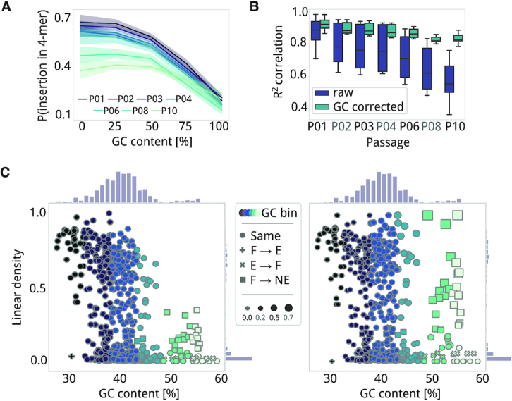
Corrections of GC content bias. (A) Average frequency (line) and standard deviation (shadow) of each DNA 4-mer having a transposon insertion as a function of GC content (X-axis). Data is presented for each passage of the U0_PE1 dataset and shows that insertion probability is higher for 4-mers with lower GC content. (B) Boxplot representing the contribution of GC bias per passage, measured as the Pearson's R² correlation between available 4-mers and disrupted 4-mers. Raw profiles of insertions are shown in purple and ANUBIS-corrected profiles in blue. (C) Scatter plots (with histograms) of linear density as a function of percentage of GC content for each annotated gene in M. pneumoniae, before (left) and after (right) correcting for GC bias by Conditional Quantile Normalization. The legends is shared between the two panels, and a gradient from black to light green represents the following GC content (% units) bins: <32, 32–38, 38–43, 43–48, 48–53, >53 (minimum number of bins with >25 genes each). Changes between essentiality categories, as estimated by GMM with components, before and after correction are labeled with the following symbols: a dot for no change, a plus sign for F to E, a cross for E to F, and a square for F to NE. The symbol size represents the difference in terms of linear density between the corrected and non-corrected values.

We also evaluated the impact of sequence composition biases at the annotation level and on essentiality estimation using P02, replica 1, as an example. When relating linear density with GC content for each gene in M. pneumoniae (genomic GC content of 40%; Figure 4C), we observed that almost all genes with a GC content ≤30% had more than 75% of their positions disrupted (28 out of 31 genes presented an average linear density of 85%). For genes with a GC content ≥50%, we observed significantly lower densities (average linear density of 27%; Wilcoxon signed-rank test; P = 0.00). While in the first case we do not expect an impact on the essentiality estimation of AT-rich genes, we could be underestimating the number of NE genes with high GC content. In fact, when running a sliding window approach comparing gene local linear densities, we observed a clear anticorrelation with the percentage of GC (Supplementary Figure S6). ANUBIS implements a Conditional Quantile Normalization (CQN) method, validated to correct biases in sequencing processes (47). This method corrects linear densities assuming full linear density for non-coding regions and using quantile normalization conditioned by GC content and linear regression correction. As changes between GC bias-corrected and non-corrected linear density were small (Pearson's R² = 0.95; P = 0.002), we observed few differences in the predicted categories when estimating essentiality (Supplementary Table S5). Looking at GMM with three components for example, only 45 genes presented different category estimations due to an increased linear density after correction. These genes have a high GC content (48–54% and >54%). Fourteen genes were corrected from E to F and 31 from F to NE, indicating that their linear density values without correction could have been underestimated. No differences were observed in terms of accuracy or NE accuracy. GC content can be very different depending on the model organism and this kind of corrections could not be appropriate for those cases. However, this correction looks to ensure there are no unbalanced linear densities distributions by GC content and it should be generally effective in other models (see Supplementary).

Correlations at the base pair level: target site duplications (TSD)

Some transposases produce staggered cuts, and as a result, cause duplication of a fixed number of nucleotide bases during the repair process (20). For a given insertion event, each of the flanking IR is followed by two different chromosome coordinates, and apparently for short read aligners, two different insertion positions. We evaluated biases at the nucleotide level by correlating read count values (i.e. a representation of a clone in the library) between insertion events and contiguous positions. The most noticeable correlation was between positions n + 7 and n - 7, a feature conserved in all passage conditions (Pearson's R² > 0.5, Supplementary Table S6; Figure 5A). This suggests that the Tn4001 transposase produces a 7-bp TSD. Considering the typical primer for PCR enrichment, which is designed to amplify the sequence from the IR to the contiguous genomic region (see Material and Methods, see Supplementary Figure S1), we deducted forward-oriented (fw) mapped reads would always cover one side of the insertion while reverse-oriented (rv) reads would cover the other. In our case, insertions detected in rv reads corresponded to the same fw profile but were shifted by +7 (Pearson's R² >0.8 for the position n + 7; Figure 5A). This effect is related to the read count that is associated with each insertion because correlation with the +7 position became significant for those positions with a read count over the 90th percentile in the general read count distribution (Pearson's R² > 0.75; P < 0.005 in all passages, Supplementary Table S7; Figure 5B). This means that TSD are more probable to be detected when transposition occurs at an NE position (i.e. clones higher read count). In F regions, however, the read count will be lower and one of the two insertions could be missing and therefore only be counted one. Using the previous observations, we defined a correction that overlaps fw and rv insertion profiles, but shifting the rv positions by +7 if their read counts are over the 90th percentile (Figure 5A).

Figure 5.

Read count correlation at the nucleotide level. (A) Schema of how TSD causes read aligners to count for the same insertion twice. When we count for regular paired-end reads mapping (first row), at the genome level (left column), the IR sequencing primer (green and purple arrows) extend from two different positions. At the sequencing level (center column), aligners like Bowtie2 will assign the insertion to two positions with a distance that is equal to the size of duplication. At the data level (right column line plots), we show the average Pearson's R² correlation between relative positions for each passage (gradient of colors). The X-axes represent a relative insertion in the center and Y-axis correlation in R² values to contiguous up- and downstream positions. (B) Exploring the correlation at the level of read count percentile (X-axis) shows that Pearson's R² correlation (Y-axis) becomes relevant when the read count of insertions falls above the 90th percentile for each passage (gradient of colors).

We applied the correction for TSD to sample P02, replica 1, and estimated essentiality using the GMM model with three components. We observed 19 genes changing categories after correction: four moving from F to E and 15 from NE to F (Supplementary Table S5). Interestingly, despite not observing changes in terms of accuracy and NE accuracy, we could be improving the estimate of F genes. With no correction, GMM properly classified two out of six genes that could be considered as F in our validation set because deleting them confers a ‘slow’ growth phenotype to M. pneumoniae (see Materials and Methods; Supplementary Table S3). With the correction, all six genes were predicted as F.

Differential essentiality regions: N- and C-termini, repeated regions and protein domains

It is known that some coding genes can tolerate transposon insertions in the extreme N- and C-termini of their ORF because the insertions are not expected to disrupt the functional core of the encoded protein (9,11). Previous studies have corrected for this by arbitrarily trimming 5% off each terminal region and considering only the inner 90% region (7,28). More aggressive filters have been applied in some studies (e.g. removing 5% from the N-terminus and 20% from C-terminus (48)). These numbers are rather arbitrary and could impact essentiality estimates. We implemented a Change Point Detection (CPD) algorithm in ANUBIS that automatically analyzes the linear density of a gene by windows to detect significant changes (39). This enables estimation of the best points (change points) delimiting the NE N- and C-termini regions of E genes that could have a different insertion profile to the rest of the gene. For example, taking the annotation of M. pneumoniae and all passages as input, we determined the average change points to be at 8% from the N-terminus and 10% from the C-terminus. In P10 for E genes, we detected the average change points at 3% and 4% for N- and C-terminal regions, respectively, indicating that they still conserve insertions at their terminal regions even after multiple selection passages. In general, the extension of NE terminal regions for E and F genes becomes shorter with each cell passage. For example, mpn116 is predicted to be a F gene (Poisson model, default) up to P06, at which point it starts to be classified as E using the arbitrary threshold of 5% from each termini. We analyzed this specific case and determined that, at P01, the first half of the protein is labeled as E while the second half is labeled as NE (Figure 6A). The differential NE region is maintained from P02 to P06, where it becomes reduced to the last 18% of the gene; being further reduced to 8% and 5% in P08 and P10, respectively. This effect was also observed for other genes, both in the N- and C-termini, indicating a progressive negative trend when insertions are further away from the N- and C-termini. Using P02 as a reference and the Poisson model as an example, we evaluated the effect of not filtering the terminal regions on predicting essentiality (arbitrary 5% cutoff and CPD methodology). Using different filters, we observed no difference in accuracy along passages. However, we did observe 61 genes changing categories when comparing the 5% termini removal versus the CPD approach. For example, genes like mpn154, mpn214 and mpn339 were labeled as F when no filter or the arbitrary 5% cutoff filter was applied, but labeled as E when using CPD (Figure 6B, Supplementary Table S5).

Figure 6.

Insertion profiles for different genes. The genome coordinates of each gene are shown on the X-axis. Gene coordinates are delimited by start (solid vertical grey line) and stop (solid vertical black line) codon positions and their respective shifted position in the 5% N- and C-terminals (dashed lines). In every plot is shown the smoothed 20-bp distribution of read count per insertion (line) passed onto the CPD algorithm. Base-pair scales are shown below the gene name. (A) Gene mpn116 at different passages, for passages 02, 06 and 08 (darker to lighter colors), presents and extended C-terminal of 50% (passage 1 and 2) that becomes shorter with selection (∼15% for P02–P06; for 5% P08 and P10). (B) E genes with extended NE N’ and C’-termini at P02. Top profile represents mpn154, which present insertions (solid blue vertical lines) in an extended C-terminal covering 23% of its length (purple box). In the middle, mpn214 has an extended N-terminal region covering 13% of the protein (blue box) and a C-terminal region of 7% (purple box). The bottom profile represents mpn339, which has a shorter N-terminal region (3%) but a longer C-terminal region (18%). (C) Genes with repeated regions at P02. Examples of potential F/NE genes (mpn141 and mpn142) that are predicted to be E when including repeated positions in the estimation (grey boxes). (D) Mpn030 at P02. This gene is a NusB-like protein with a dispensable N’-terminal. Insertions before amino acid 58 still enable the expression of a functional, shorter version of the protein because of an internal start codon (labeled with blue arrow) that still expresses the domain of the protein found conserved by HMMER.

The CPD algorithm also enables the automatic detection of cases in which a protein comprises multiple differential essential domains. We hypothesized that E domains within apparently NE genes could either be the result of repeated loci in the genome preventing the mapping of insertions (ambiguously mapped reads are generally counted separately by read aligners like Bowtie2) or a specific functional domain in the protein that, unlike the rest of the gene, is essential (7). To test the first hypothesis, we generated a reference of repetitive DNA sequences in M. pneumoniae M129 and observed that mapping was efficient for repeated regions shorter than 100 bases, independent of the passage number (Supplementary Figure S7, Supplementary Data 2). Hence, repeated regions longer than 100 bases are ignored by ANUBIS when calculating metrics such as linear density. For the latter hypothesis about protein domains, ANUBIS was designed to accept additional annotations such as HMMER protein domain predictions (49) and report differential essentiality assignments between those domains and the general gene. We tested the impact of these two types of regions on protein essentiality using the Poisson model along different passages. We observed minimal differences along passages, with only 10–15 genes changing category per passage. Despite most changes being between the F and NE categories, some interesting cases arose including mpn141 and mpn142 (Figure 6C). These genes were predicted as E in every passage condition when including repeated regions but predicted as F after correction (Supplementary Table S5). In fact, spontaneous mutants for these cytadherence-related genes have been isolated, demonstrating they are dispensable for in vitro growth conditions (50). Therefore, these results indicate that if repeated regions are considered, specific disruptable genes in an organism could be hidden. In addition, when looking for different essential HMMER domains, we found genes with apparent local differences in terms of linear density. However, all these cases could be explained by the protein having extended N’ and C’-terminal NE regions, or E regions derived from repeated regions. Interestingly, while mpn030 (168 amino acids), which has structural homology to NusB proteins (51), presented an enrichment in linear density from amino acid positions 13–53, the rest of the protein (corresponding to HMMER domain DUF1948) had no insertions. Interestingly, mpn030 has an alternative start codon (GTG) after that specific NE region, suggesting this gene is essential with an NE N-terminal region not required for cell viability (Figure 6D). This is supported by the fact orthologs of mpn030 in other mycoplasmas do not present any extension. This could be an effect derived from the acquisition during evolution of an ATG start codon (preferred over GTG), which adds ∼50 amino acids without affecting the original protein functionality.

Effect of coverage, methodology and corrections on predicting gene essentiality

We performed a general evaluation of models by examining how linear density is affected by transposon coverage and different estimate parameters (Figure 1E and Supplementary Data 3; see Materials and Methods). This analysis is important because in vivo essentiality studies, for example, result in a much lower transposon insertion density than in vitro studies due to stronger sampling and selection conditions. Also, we could have lower coverages when we analyzing larger genomes like Escherichia coli (4,000 kb) where transposon insertion saturation is harder to achieve. We first explored how accuracy is related to the coverage reduction that is produced by continuous selection (i.e. over passages). We observed that a genome coverage of at least 10% (10 insertions every 100 bp) is required to provide accurate estimates of both accuracy and NE accuracy. As described above, estimates made by Gumbel, GMM, and BGMM outperformed estimates made by Poisson and Gamma models independently to the filters and processing steps had been applied (Figure 7A and B).

Figure 7.

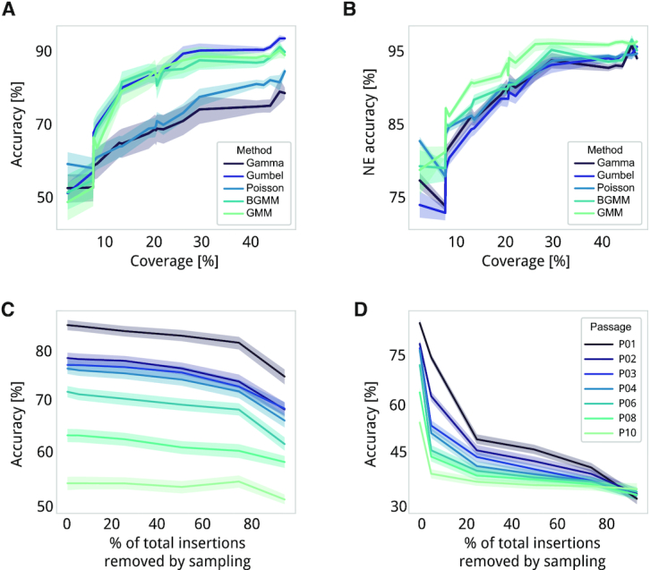
Comparison of essentiality estimates for different passages and different parameterizations. (A) Line plots representing accuracy and (B), NE accuracy for each coverage found in our dataset). Solid lines represent the average accuracy of each model (different gradient colors) and shadows represent the expected variability as standard deviation. (C) Impact of randomly removing insertions on accuracy. The X-axis represents the sampling level, or the percentage of inserted positions in the sample that are randomly removed. Solid lines represent each of the samples (different gradient colors) and shadows represent the expected variability as standard deviation. (D) Same as panel c but with the sampling method based on read count values (e.g. at 75% we consider only those insertions with a read count >75th percentile of the total read distribution).

Secondly, we artificially produced a sampling effect by randomly removing insertions from a profile in a sequential and controlled manner (Figure 1E; see Materials and Methods). We were able to randomly remove up to 75% of the insertions in a dataset without losing accuracy. This indicates that sampling effects that occur during passages (i.e. dilution of cell populations performed between each passage) do not account for large differences in essentiality estimates (Figure 7C) but it could affect specific annotations (e.g. short ones, see Supplementary). Additionally, we explored with a sampling method based on subsequently increasing a read count threshold (Figure 1E). We found that positions with a read count below the 5th percentile are required for proper estimation of essentiality based on our validation set. In each sample, the 5th percentiles corresponded to a read count of 3–4, indicating that most of these low read insertions are real despite the fact that they can be caused by artifactual factors such as the ones described above (Figure 7D). However, it is common to find insertions with a read count of ≤2 in E genes. Thus, we considered three different types of read filters in the comparative iterations: (i) removing positions with a read count of ≤2, (ii) trimming 5% of the read count distribution from the top and bottom (i.e. ‘tails’) (28) and (iii) filtering out insertions with read values in the range of read counts mapped to know or validated E genes (i.e consider those insertions as ‘noise’ derived from dead cells or mismapped positions, see Materials and Methods).

Lastly, we explored the variation in accuracy produced by each preprocessing mode, including models, the three different read threshold filters mentioned above, corrections for repeated, TSD, N- and C-terminal extended regions, criteria used for assigning essentiality categories, and definitions of expected NE linear density from the gold standard set or non-coding regions (Supplementary Figure S8). As already mentioned, Gumbel, GMM and BGMM models presented the best overall accuracy, with BGMM showing considerably less variability than other Materials and Methods. With respect to filtering by read counts, we observed that removing insertions with a read count smaller than 3 was beneficial when estimating essentiality, improving estimation of E genes and F genes in the validation set, but at the cost of accuracy in detecting NE genes. The accuracy in detecting NE genes also decreased, albeit more aggressively, when applying filters based on E genes or removing tails (Supplementary Figure S8). Correcting for repeated regions, TSD artifacts, and the use of a CPD-based definition of N- and C-termini did not improve overall accuracy (Supplementary Figure S8). However, we already described how these corrections were beneficial for specific genes. Similar as when correcting for GC biases, these corrections should be specifically applied at the gene level. Finally, for Poisson, Gumbel and Gamma models we evaluated different gold standard sets, and class criteria definition (see the last two sections in Material and Methods; see Table 3). We found that the best criterion for estimating essentiality with these models is the fold change (FC) between E and NE probabilities, where log₂FC<2 = NE and log₂FC>2 = E (Supplementary Figure S8). For GMM and BGMM models, we found that two components provided the best accuracy, although this is at the cost of losing the F category. With respect to the gold standard set, estimating the expected linear density of NE genes from non-coding regions provided more accurate estimates than using a user-defined gold standard set (Supplementary Figure S8).

Overall, estimation of essentiality is a complex task that requires multiple evaluation steps and consideration of factors that, despite not introducing dramatic changes in the general assessment of essentiality, can lead to the incorrect estimation of a specific set of genes. ANUBIS includes all the necessary functions to run Tn-seq data analyses from scratch so that the user can visually and analytically explore the impact of each of the introduced corrections.

DISCUSSION

Here, we first presented FASTQINS, a pipeline able to extract transposon insertion profiles from sequencing data. FASTQINS considers available experimental and design conditions, accepting multiple input types to deliver results in a standardized format. We complemented it with ANUBIS, a Python standalone framework that helps to detect and correct factors that can cause deviations in essentiality estimates. ANUBIS combines, in a single tool, state-of-the-art Tn-seq analysis approaches, with new corrections for previously unconsidered factors, and novel models that do not require any previous knowledge on the essentiality of the organism considered. We have discussed factors that greatly affect essentiality estimates, including TSD, PCR duplicates, GC bias, differential domains, and essentiality estimate models. We conclude that Tn-seq is a highly sensitive protocol that requires additional processing steps (compared to techniques such as DNA-seq and RNA-seq) and controlled supervision to retrieve accurate estimates. In this respect, ANUBIS provides routines and visualizations to guide along the best processing steps to use before predicting essentiality. Additionally, the user experimental design makes necessary specific considerations and correction/processing steps. For example, users can explore profiles at the level of insertion read counts (e.g. using HMM). If this is the case, we recommend performing minimal passages (≤30 cell divisions in our case) and PCR duplicates, GC content bias and TSD are highly recommended to be considered. When a more general perspective is desired (e.g. in gene essentiality studies), we found that to obtain good estimates a minimum genome transposon coverage of 10% is required, and that repeated regions and limits for NE N- or C-terminal regions should be properly assigned. ANUBIS also provides all the necessary tools to statistically and visually evaluate whether a gene can be removed from an organism or not, thereby aiding in the rational design of genome reductions. Ultimately, ANUBIS collects functions to fit, predict, report, and visualize the estimation results using different models. It implements previously described estimators based on Poisson, Gumbel, Gamma and HMM models allowing the user to run previously described essentiality models. While these models have been proved to be useful in their original references, they present the limitation of depending on training sets, not always accessible for an organism of interest. This motivated us to implement unsupervised models based on mixture models such as GMM and BGMM that we believe can be useful in organisms with little knowledge about gene essentiality and/or gene function. Altogether, we envision ANUBIS as a computational and customizable framework that can perform Tn-seq data treatments, benchmark essentiality studies or be integrated into larger analysis pipelines. Essentiality estimation is a complex task where multiple factors have to be taken into consideration and the requirements of the user can be very different. Thus, in ANUBIS all the corrections are optional and is the user who decides which of them have to be applied supported by visual and statistical exploration. However, it also includes specific procedures to automate these corrections based on statistical assumptions for those users with little background in essentiality studies. Both tools have been developed integrating available bioinformatic standards as well as general statistical assumptions that makes it possible to apply them to other organisms. This is important as factors presented here could present different impacts depending on the study species. Nowadays, in the era of Synthetic Biology, a Tn-seq experiment processed by FASTQINS and explored and analyzed using ANUBIS, provides a perfect starting point to define the essential core machinery and elements that can be removed from a model organism in a sensitive and accurate manner. This, coupled together with targeted editing methodologies (e.g. CRISPR/Cas9 system), can represent a step forward in the rational design of genome-reduced organisms and biological chassis that have important biotechnological and/or biomedical applications.

DATA AVAILABILITY

The code and manuals for the two tools presented in this study can be downloaded as standalone applications or as Python packages from https://github.com/CRG-CNAG/fastqins and https://github.com/CRG-CNAG/anubis.

Tn-seq raw data files have been deposited in the ArrayExpress database at EMBL-EBI, under accession number E-MTAB-8918, and are accessible from the following link: http://www.ebi.ac.uk/arrayexpress/experiments/E-MTAB-8918.

SUPPLEMENTARY DATA

Supplementary Data are available at NAR Online.

FUNDING

ERASynBio 2nd Joint Call for Transnational Research Projects: ‘Building Synthetic Biology Capacity Through Innovative Translational Projects’, with funding from the corresponding ERASynBio National Funding Agencies; European Research Council (ERC) under the European Union's Horizon 2020 research and innovation program [670216] (MYCOCHASSIS); CERCA Programme/Generalitat de Catalunya; Spanish Ministry of Science and Innovation to the EMBL partnership, ‘Centro de Excelencia Severo Ochoa 2013–2017’. Funding for open access charge: ERASynBio 2nd Joint Call for Transnational Research Projects: ‘Building Synthetic Biology Capacity Through Innovative Translational Projects’, with funding from the corresponding ERASynBio National Funding Agencies; European Research Council (ERC) under the European Union's Horizon 2020 research and innovation program [670216] (MYCOCHASSIS); CERCA Programme/Generalitat de Catalunya; Spanish Ministry of Science and Innovation to the EMBL partnership, ‘Centro de Excelencia Severo Ochoa 2013–2017’

Conflict of interest statement. None declared.

REFERENCES

- 1. Chi H., Wang X., Shao Y., Qin Y., Deng Z., Wang L., Chen S.. Engineering and modification of microbial chassis for systems and synthetic biology. Synth. Syst. Biotechnol. 2019; 4:25–33. [DOI] [PMC free article] [PubMed] [Google Scholar]
- 2. Salama N.R., Shepherd B., Falkow S.. Global transposon mutagenesis and essential gene analysis of Helicobacter pylori. J. Bacteriol. 2004; 186:7926–7935. [DOI] [PMC free article] [PubMed] [Google Scholar]
- 3. Wong S.M.S., Gawronski J.D., Lapointe D., Akerley B.J.. High-throughput insertion tracking by deep sequencing for the analysis of bacterial pathogens. Methods Mol. Biol. 2011; 733:209–222. [DOI] [PubMed] [Google Scholar]
- 4. Green B., Bouchier C., Fairhead C., Craig N.L., Cormack B.P.. Insertion site preference of Mu, Tn5, and Tn7 transposons. Mob. DNA. 2012; 3:3. [DOI] [PMC free article] [PubMed] [Google Scholar]
- 5. Arenas J., Zomer A., Harders-Westerveen J., Bootsma H.J., De Jonge M.I., Stockhofe-Zurwieden N., Smith H.E., De Greeff A.. Identification of conditionally essential genes for Streptococcus suis infection in pigs. Virulence. 2020; 11:446–464. [DOI] [PMC free article] [PubMed] [Google Scholar]
- 6. van Opijnen T., Bodi K.L., Camilli A.. Tn-seq: high-throughput parallel sequencing for fitness and genetic interaction studies in microorganisms. Nat. Methods. 2009; 6:767–772. [DOI] [PMC free article] [PubMed] [Google Scholar]
- 7. Lluch-Senar M., Delgado J., Chen W.-H., Lloréns-Rico V., O’Reilly F.J., Wodke J.A., Unal E.B., Yus E., Martínez S., Nichols R.J. et al.. Defining a minimal cell: essentiality of small ORFs and ncRNAs in a genome-reduced bacterium. Mol. Syst. Biol. 2015; 11:780. [DOI] [PMC free article] [PubMed] [Google Scholar]
- 8. Barquist L., Mayho M., Cummins C., Cain A.K., Boinett C.J., Page A.J., Langridge G.C., Quail M.A., Keane J.A., Parkhill J.. The TraDIS toolkit: sequencing and analysis for dense transposon mutant libraries. Bioinformatics. 2016; 32:1109–1111. [DOI] [PMC free article] [PubMed] [Google Scholar]
- 9. Langridge G.C., Phan M.-D., Turner D.J., Perkins T.T., Parts L., Haase J., Charles I., Maskell D.J., Peters S.E., Dougan G. et al.. Simultaneous assay of every Salmonella Typhi gene using one million transposon mutants. Genome Res. 2009; 19:2308–2316. [DOI] [PMC free article] [PubMed] [Google Scholar]
- 10. Glass J.I., Assad-Garcia N., Alperovich N., Yooseph S., Lewis M.R., Maruf M., Hutchison C.A., Smith H.O., Venter J.C.. Essential genes of a minimal bacterium. Proc. Natl. Acad. Sci. U.S.A. 2006; 103:425–430. [DOI] [PMC free article] [PubMed] [Google Scholar]
- 11. Akerley B.J., Rubin E.J., Camilli A., Lampe D.J., Robertson H.M., Mekalanos J.J.. Systematic identification of essential genes by in vitro mariner mutagenesis. Proc. Natl. Acad. Sci. U.S.A. 1998; 95:8927–8932. [DOI] [PMC free article] [PubMed] [Google Scholar]
- 12. Iii C.A.H., Hutchison C.A. III. Global transposon mutagenesis and a minimal mycoplasma genome. Science. 1999; 286:2165–2169. [DOI] [PubMed] [Google Scholar]
- 13. Parekh S., Ziegenhain C., Vieth B., Enard W., Hellmann I.. The impact of amplification on differential expression analyses by RNA-seq. Sci. Rep. 2016; 6:25533. [DOI] [PMC free article] [PubMed] [Google Scholar]
- 14. Li H., Handsaker B., Wysoker A., Fennell T., Ruan J., Homer N., Marth G., Abecasis G., Durbin R. 1000 Genome Project Data Processing Subgroup . The sequence Alignment/Map format and SAMtools. Bioinformatics. 2009; 25:2078–2079. [DOI] [PMC free article] [PubMed] [Google Scholar]
- 15. Xu H., Luo X., Qian J., Pang X., Song J., Qian G., Chen J., Chen S.. FastUniq: A fast de novo duplicates removal tool for paired short reads. PLoS One. 2012; 7:e52249. [DOI] [PMC free article] [PubMed] [Google Scholar]
- 16. Laehnemann D., Borkhardt A., McHardy A.C.. Denoising DNA deep sequencing data-high-throughput sequencing errors and their correction. Brief. Bioinform. 2016; 17:154–179. [DOI] [PMC free article] [PubMed] [Google Scholar]
- 17. Wetmore K.M., Price M.N., Waters R.J., Lamson J.S., He J., Hoover C.A., Blow M.J., Bristow J., Butland G., Arkin A.P. et al.. Rapid quantification of mutant fitness in diverse bacteria by sequencing randomly bar-coded transposons. MBio. 2015; 6:e00306–15. [DOI] [PMC free article] [PubMed] [Google Scholar]
- 18. Plasterk R.H., Izsvák Z., Ivics Z.. Resident aliens: the Tc1/mariner superfamily of transposable elements. Trends Genet. 1999; 15:326–332. [DOI] [PubMed] [Google Scholar]
- 19. Goryshin I.Y., Miller J.A., Kil Y.V., Lanzov V.A., Reznikoff W.S.. Tn5/IS50 target recognition. Proc. Natl. Acad. Sci. U.S.A. 1998; 95:10716–10721. [DOI] [PMC free article] [PubMed] [Google Scholar]
- 20. Levin H.L., Moran J.V.. Dynamic interactions between transposable elements and their hosts. Nat. Rev. Genet. 2011; 12:615–627. [DOI] [PMC free article] [PubMed] [Google Scholar]
- 21. Han M.-J., Xu H.-E., Zhang H.-H., Feschotte C., Zhang Z.. Spy: a new group of eukaryotic DNA transposons without target site duplications. Genome Biol. Evol. 2014; 6:1748–1757. [DOI] [PMC free article] [PubMed] [Google Scholar]
- 22. Bolstad B.M., Irizarry R.A., Astrand M., Speed T.P.. A comparison of normalization methods for high density oligonucleotide array data based on variance and bias. Bioinformatics. 2003; 19:185–193. [DOI] [PubMed] [Google Scholar]
- 23. DeJesus M.A., Ioerger T.R.. Normalization of transposon-mutant library sequencing datasets to improve identification of conditionally essential genes. J. Bioinform. Comput. Biol. 2016; 14:1642004. [DOI] [PMC free article] [PubMed] [Google Scholar]
- 24. DeJesus M.A., Zhang Y.J., Sassetti C.M., Rubin E.J., Sacchettini J.C., Ioerger T.R.. Bayesian analysis of gene essentiality based on sequencing of transposon insertion libraries. Bioinformatics. 2013; 29:695–703. [DOI] [PMC free article] [PubMed] [Google Scholar]
- 25. Osterman A.L., Gerdes S.Y.. Microbial Gene Essentiality: Protocols and Bioinformatics. 2010; Humana Press. [Google Scholar]
- 26. DeJesus M.A., Ioerger T.R.. A Hidden Markov Model for identifying essential and growth-defect regions in bacterial genomes from transposon insertion sequencing data. BMC Bioinformatics. 2013; 14:303. [DOI] [PMC free article] [PubMed] [Google Scholar]
- 27. McCoy K.M., Antonio M.L., van Opijnen T.. MAGenTA: a Galaxy implemented tool for complete Tn-Seq analysis and data visualization. Bioinformatics. 2017; 33:2781–2783. [DOI] [PMC free article] [PubMed] [Google Scholar]
- 28. DeJesus M.A., Ambadipudi C., Baker R., Sassetti C., Ioerger T.R.. TRANSIT–a software tool for Himar1 TnSeq analysis. PLoS Comput. Biol. 2015; 11:e1004401. [DOI] [PMC free article] [PubMed] [Google Scholar]
- 29. Veeranagouda Y., Didier M.. Transposon Insertion Site Sequencing (TIS-Seq): an efficient and high-throughput method for determining transposon insertion site(s) and their relative abundances in a PiggyBac transposon mutant pool by next-generation sequencing. Current Protocols in Molecular Biology. 2017; 21.35.1–21.35.11. [DOI] [PubMed] [Google Scholar]
- 30. Güell M., van Noort V., Yus E., Chen W.-H., Leigh-Bell J., Michalodimitrakis K., Yamada T., Arumugam M., Doerks T., Kühner S. et al.. Transcriptome complexity in a genome-reduced bacterium. Science. 2009; 326:1268–1271. [DOI] [PubMed] [Google Scholar]
- 31. Yus E., Maier T., Michalodimitrakis K., van Noort V., Yamada T., Chen W.-H., Wodke J.A.H., Güell M., Martínez S., Bourgeois R. et al.. Impact of genome reduction on bacterial metabolism and its regulation. Science. 2009; 326:1263–1268. [DOI] [PubMed] [Google Scholar]
- 32. Weber M., Burgos R., Yus E., Yang J.-S., Lluch-Senar M., Serrano L.. Impact of C-terminal amino acid composition on protein expression in bacteria. Mol. Syst. Biol. 2020; 16:e9208. [DOI] [PMC free article] [PubMed] [Google Scholar]
- 33. Burgos R., Totten P.A.. Characterization of the operon encoding the Holliday junction helicase RuvAB from Mycoplasma genitalium and its role in mgpB and mgpC gene variation. J. Bacteriol. 2014; 196:1608–1618. [DOI] [PMC free article] [PubMed] [Google Scholar]
- 34. Pich O.Q., Burgos R., Planell R., Querol E., Piñol J.. Comparative analysis of antibiotic resistance gene markers in Mycoplasma genitalium: application to studies of the minimal gene complement. Microbiology. 2006; 152:519–527. [DOI] [PubMed] [Google Scholar]
- 35. Langmead B., Salzberg S.L.. Fast gapped-read alignment with Bowtie 2. Nat. Methods. 2012; 9:357–359. [DOI] [PMC free article] [PubMed] [Google Scholar]
- 36. Li H., Handsaker B., Wysoker A., Fennell T., Ruan J., Homer N., Marth G., Abecasis G., Durbin R. 1000 Genome Project Data Processing Subgroup . The sequence Alignment/Map format and SAMtools. Bioinformatics. 2009; 25:2078–2079. [DOI] [PMC free article] [PubMed] [Google Scholar]
- 37. Quinlan A.R., Hall I.M.. BEDTools: a flexible suite of utilities for comparing genomic features. Bioinformatics. 2010; 26:841–842. [DOI] [PMC free article] [PubMed] [Google Scholar]
- 38. Goodstadt L. Ruffus: a lightweight Python library for computational pipelines. Bioinformatics. 2010; 26:2778–2779. [DOI] [PubMed] [Google Scholar]
- 39. Truong C., Oudre L., Vayatis N.. Selective review of offline change point detection methods. Signal Process. 2020; 167:107299. [Google Scholar]
- 40. Charbonneau A.R.L., Forman O.P., Cain A.K., Newland G., Robinson C., Boursnell M., Parkhill J., Leigh J.A., Maskell D.J., Waller A.S.. Defining the ABC of gene essentiality in streptococci. BMC Genomics. 2017; 18:426. [DOI] [PMC free article] [PubMed] [Google Scholar]
- 41. Yus E., Lloréns-Rico V., Martínez S., Gallo C., Eilers H., Blötz C., Stülke J., Lluch-Senar M., Serrano L.. Determination of the gene regulatory network of a Genome-Reduced bacterium highlights alternative regulation independent of transcription factors. Cell Syst. 2019; 9:143–158. [DOI] [PMC free article] [PubMed] [Google Scholar]
- 42. Garreta R., Moncecchi G.. Learning scikit-learn: Machine Learning in Python. 2013; Packt Publishing Ltd. [Google Scholar]
- 43. Akaike H. Parzen E., Tanabe K., Kitagawa G.. Information theory and an extension of the maximum likelihood principle. Selected Papers of Hirotugu Akaike. 1992; Springer SeriesStatistics; 199–213. [Google Scholar]
- 44. Poulsen B.E., Yang R., Clatworthy A.E., White T., Osmulski S.J., Li L., Penaranda C., Lander E.S., Shoresh N., Hung D.T.. Defining the core essential genome of. Proc. Natl. Acad. Sci. U.S.A. 2019; 116:10072–10080. [DOI] [PMC free article] [PubMed] [Google Scholar]
- 45. Chao M.C., Abel S., Davis B.M., Waldor M.K.. The design and analysis of transposon insertion sequencing experiments. Nat. Rev. Microbiol. 2016; 14:119–128. [DOI] [PMC free article] [PubMed] [Google Scholar]
- 46. Kumar A., Seringhaus M., Biery M.C., Sarnovsky R.J., Umansky L., Piccirillo S., Heidtman M., Cheung K.-H., Dobry C.J., Gerstein M.B. et al.. Large-scale mutagenesis of the yeast genome using a Tn7-derived multipurpose transposon. Genome Res. 2004; 14:1975–1986. [DOI] [PMC free article] [PubMed] [Google Scholar]
- 47. Hansen K.D., Irizarry R.A., Wu Z.. Removing technical variability in RNA-seq data using conditional quantile normalization. Biostatistics. 2012; 13:204–216. [DOI] [PMC free article] [PubMed] [Google Scholar]
- 48. Gawronski J.D., Wong S.M.S., Giannoukos G., Ward D.V., Akerley B.J.. Tracking insertion mutants within libraries by deep sequencing and a genome-wide screen for Haemophilus genes required in the lung. Proc. Natl. Acad. Sci. U.S.A. 2009; 106:16422–16427. [DOI] [PMC free article] [PubMed] [Google Scholar]
- 49. Finn R.D., Clements J., Eddy S.R.. HMMER web server: interactive sequence similarity searching. Nucleic Acids Res. 2011; 39:W29–W37. [DOI] [PMC free article] [PubMed] [Google Scholar]
- 50. Balish M.F., Ross S.M., Fisseha M., Krause D.C.. Deletion analysis identifies key functional domains of the cytadherence-associated protein HMW2 of Mycoplasma pneumoniae. Mol. Microbiol. 2003; 50:1507–1516. [DOI] [PubMed] [Google Scholar]
- 51. Liu J., Yokota H., Kim R., Kim S.-H.. A conserved hypothetical protein from mycoplasma genitalium shows structural homology to nusb proteins. Proteins. 2004; 55:1082–1086. [DOI] [PubMed] [Google Scholar]
Associated Data
This section collects any data citations, data availability statements, or supplementary materials included in this article.
Supplementary Materials
Data Availability Statement