Highlights
-
•
Corona virus,
-
•
Reported and unreported cases,
-
•
Isolation, quarantine, public closings;
-
•
Epidemic mathematical model
Keywords: Corona virus, Reported and unreported cases, Isolation, Quarantine, Public closings, Epidemic mathematical model
Abstract
We model the COVID-19 coronavirus epidemics in China, South Korea, Italy, France, Germany and the United Kingdom. We identify the early phase of the epidemics, when the number of cases grows exponentially, before government implementation of major control measures. We identify the next phase of the epidemics, when these social measures result in a time-dependent exponentially decreasing number of cases. We use reported case data, both asymptomatic and symptomatic, to model the transmission dynamics. We also incorporate into the transmission dynamics unreported cases. We construct our models with comprehensive consideration of the identification of model parameters. A key feature of our model is the evaluation of the timing and magnitude of implementation of major public policies restricting social movement. We project forward in time the development of the epidemics in these countries based on our model analysis.
1. Introduction
COVID-19 epidemics are currently a global crisis. Our goal in this paper is to develop a mathematical model to guide understanding of the dynamics of COVID-19 epidemics. In previous works (Liu et al., 2020, Liu et al., 2020, Liu et al., 2020), our team has developed differential equations models of COVID-19 epidemics. Our goal is to predict forward in time the future number of cases from early reported case data in regions throughout the world. Our model incorporate the following important elements of COVID-19 epidemics: (1) the number of asymptomatic infectious individuals (with no or very mild symptoms), (2) the number of symptomatic reported infectious individuals (with severe symptoms) and (3) the number of symptomatic unreported infectious individuals (with mild symptoms). With our model, we provide a prediction of the final size of the asymptomatic infectious cases, the reported cases (with severe symptoms) and unreported cases (with mild symptoms). We will apply the model in this paper to the epidemics in China, South Korea, Italy, France, Germany, and the United Kingdom.
The significance of transmission by asymptomatic and mildly symptomatic individuals is of major importance. It is well established that newly infected patients, who are asymptomatic or have only mild symptoms, can transmit the virus (Guan et al., 2019, Mizumoto et al., 2019, Nishiura, 2020, Qiu, 2020, Rothe et al., 2019, Wang et al., 2020, Wölfel, 2020). In an early phase of the epidemic, the reported case data grows exponentially, which corresponds to a constant transmission rate. We assume that government measures and public awareness cause this early constant transmission rate to change to a time dependent exponentially decreasing rate. We identify this early constant transmission rate using a method developed in Liu et al. (2020). We then identify the time dependent exponentially decreasing transmission rate from reported case data, and project forward the time-line of the epidemic course. Our model is applicable to COVID-19 epidemics in any region with reported case data, which can be updated to higher accuracy with on-going day-by-day reported case data. We refer to Ahmed et al., 2020, Chowell and Viboud, 2016, Jajarmi et al., 2020, Kucharski et al., 2020, Mustapha, 2020, Roda et al., 2020, Verity et al., 2020 for related results.
The organisation of this paper is as follows. In Section 2 we present a general differential equations model for current COVID-19 epidemics, applicable to any region for which reported case data is available. In Section 3 we provide a general method to parameterize and initialize the model. In Section 4 we apply the model to China, South Korea, Italy, France, Germany, and the United Kingdom. In Section 5 we discuss conclusions obtained from our analysis.
2. Model
The model consists of a mass action law epidemic model where the asymptomatic infectious and the unreported infectious can transmit the virus
| (2.1) |
This system is supplemented by initial data
| (2.2) |
Here is time in days, is the beginning date from which the number of reported symptomatic infectious individuals grows exponentially, is the number of individuals susceptible to infection at time t, is the number of asymptomatic infectious individuals at time t, is the number of reported symptomatic infectious individuals at time t (i.e. symptomatic infectious with sever symptoms), and is the number of unreported symptomatic infectious individuals at time t (i.e. symptomatic infectious with mild or no symptoms).
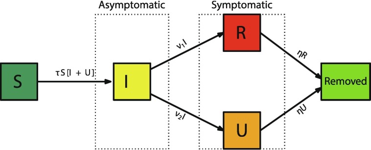
The transmission rate at time t is . Asymptomatic infectious individuals are infectious for an average period of days. Reported symptomatic individuals are infectious for an average period of days, as are unreported symptomatic individuals . We assume that reported symptomatic infectious individuals are reported and isolated immediately, and cause no further infections. The asymptomatic individuals can also be viewed as having a low-level symptomatic state. All infections are acquired from either or individuals. The fraction f of asymptomatic infectious become reported symptomatic infectious, and the fraction become unreported symptomatic infectious. The rate asymptomatic infectious become reported symptomatic is , the rate asymptomatic infectious become unreported symptomatic is , where . The cumulative number of reported cases at time t is obtained by using the following equation
| (2.3) |
and the cumulative number of unreported at time t is given by the formula
| (2.4) |
The parameters and initial conditions of the model are given in Table 1 and a flow diagram of the model is given in Fig. 1 .
Table 1.
Parameters and initial conditions of the model.
| Symbol | Interpretation | Method |
|---|---|---|
| Date from which the epidemic grows exponentially | fitted | |
| Number of susceptible at time | fixed | |
| Number of asymptomatic infectious at time | fitted | |
| Number of reported symptomatic infectious at time | fitted | |
| Number of unreported symptomatic infectious at time | fitted | |
| Transmission rate at time t | fitted | |
| N | Date at which public intervention measures became effective | fitted |
| Intensity of the public intervention measures | fitted | |
| Average time during which asymptomatic infectious are asymptomatic | fixed | |
| f | Fraction of asymptomatic infectious that become reported symptomatic infectious | fixed |
| Rate at which asymptomatic infectious become reported symptomatic | fitted | |
| Rate at which asymptomatic infectious become unreported symptomatic | fitted | |
| Average time during which symptomatic infectious have symptoms | fixed |
Fig. 1.
Compartments and flow chart of the model.
3. Method to estimate the parameters and initial conditions
We assume that of symptomatic infectious cases go unreported. The actual value of f is unknown and varies from country to country. We assume , which means that the average period of infectiousness of both unreported symptomatic infectious individuals and reported symptomatic infectious individuals is 7 days. We assume , which means that the average period of infectiousness of asymptomatic infectious individuals is 7 days. These values can be modified as further epidemiological information becomes known.
At an early stage of the epidemic we assume that all the infected components of the system grow exponentially while the number of susceptible remains unchanged during a relatively short period of time , which corresponds to a constant transmission rate . Therefore, we will assume that
| (3.1) |
We deduce that the cumulative number of reported satisfies
| (3.2) |
and by replacing by the exponential formula in (3.1), we have
| (3.3) |
Hence it makes sense to assume that has the following form
| (3.4) |
By identifying (3.3), (3.4) we deduce that
| (3.5) |
Moreover by assuming that the number of susceptible remains constant on the time interval , the I-equation, R-equation and U-equation of the model (2.1) become
By using (3.1) we obtain
Computing further, we get
| (3.6) |
By (3.5) we deduce that
| (3.7) |
Finally we obtain
| (3.8) |
The value of the basic reproductive number is
| (3.9) |
which was derived in Liu et al. (2020).
During the exponential growth phase of the epidemic, is constant. When strong government measures such as isolation, quarantine, and public closings are implemented, we use an exponential decrease for a time-dependent decreasing transmission rate to incorporate these effects since the actual effects of these measures are complex. The formula for during this phase is
| (3.10) |
The date N and the value are chosen so that the cumulative reported cases in the numerical simulation of the epidemic aligns with the cumulative reported case data after day N, when the public measures take effect. In this way we are able to project forward the time-path of the epidemic after the government imposed public restrictions take effect.
The daily number of reported cases from the model can be obtained by computing the solution of the following equation:
| (3.11) |
4. Predicting the cumulative number of cases
In this section we apply the method described in Section 3 to the data of confirmed cases in China, South Korea, Italy, France, Germany, and the United Kingdom. We predict the time evolution of a COVID-19 epidemic through its phases, we identify epidemic turning points by using the data for the cumulative number of reported cases and the daily number of reported cases, and we project the epidemic final sizes.
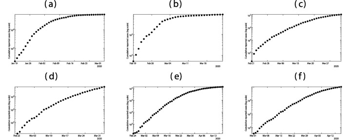
As we can see in Fig. 2 , a major difficulty for the predictions from the reported case data, is to determine the date intervals for the exponential growth phase of the epidemic. For South Korea, the date intervals for the exponential growth phase of the epidemic is relatively clear from February 25 to March 1. This is because the measures imposed for contact tracing and social distancing were very strong. For Italy, the interval is more difficult to ascertain. We choose March 1 to March 10, but these values may change as more data of reported cases becomes available. For France, Germany, and the United Kingdom, the interval is very difficult to know with the present data. Again, future reported case data, will clarify these intervals. In general, the dates for the exponential growth interval and the date N, are key elements of our model, and they depend strongly on the implementation of social distancing measures. If these measures are implemented gradually, then the difficulty is increased.
Fig. 2.
In this figure we plot the cumulative number cases (with log scale) at the early beginning of the epidemic for (a) mainland China; (b) South Korea; (c) Italy; (d) France; (e) Germany; (f) UK.
Another difficulty in applying our model is how to fix the values of the parameters . We take , which means that the average period of infectiousness of both unreported symptomatic infectious individuals and reported symptomatic infectious individuals is 7 days, , which means that the average period of infectiousness of asymptomatic infectious individuals is 7 days. These values follow from the medical and epidemiological information and can be modified as further epidemiological information becomes known. N is around the time point of the implementation of the national prevention and control measures. The values of f is unknown, but information about the level of testing relates to the value of f. A decreased value of f corresponds to a greater final size of the epidemic. The increased testing can increase the value of f. Mortality can also be used as a reference to estimate the value of f. High mortality indicates high unreported ratio. In fact, from the values of and , we can also obtain some information of the actual effects of these measures of testing, quarantining and isolation implemented by the governments in these countries.
The principle of our method is the following. By using an exponential best fit method we obtain a best fit of (3.4) to the data over a time and we derive the parameters and . The values of and are obtained by using (3.7), (3.8). Next we fix N (first day of public intervention) to some value and we obtain by trying to get the best fit to the data.
In the method the uncertainty in our prediction is due to the fact that several sets of parameters may give a good fit to the data. As a consequence, at the early stage of the epidemics (in particular before the turning point) the outcome of our method can be very different from one set of parameters to another. We try to solve this uncertainty problem by using several choices of the period to fit an exponential growth of the data to determine and and several choices for the first day of intervention N. So in this section, we vary the time interval , during which we use the data to obtain and by using an exponential fit. In the simulations below, the first day and the last day vary such that
We also vary the first day of public intervention
We vary f between to . For each we evaluate to obtain the best fit of the model to the data. We use the mean absolute deviation as the distance to data to evaluate the best fit to the data. We obtain a large number of best fit depending on and we plot smallest mean absolute deviation . Then we plot all the best fit graphs with mean absolute deviation between and .
5. Numerical simulations
The numerical simulations are presented in the chronological order of appearance for six countries (China, South Korea, Italy, France, Germany and United Kingdom). The data used are taken from URL, 2020, URL1, 2020, URL2, 2020, URL3, 2020, URL4, 2020, URL4, 2020.
5.1. Predicting the number of cases for mainland China
Before February 11, the data was based on confirmed testing. From February 11 to February 15, the data included cases that were not tested for the virus, but were clinically diagnosed. There were 17,409 such cases from February 11 to February 15 and there is a gap in the reported case data on February 11. The data from February 11 to February 15 specified both types of reported cases (i.e. the case tested for virus and the case clinically diagnosed). From February 16, the data did not separate the two types of reporting, but reported the sum of both types. We subtracted 17,409 cases (i.e. the new clinically diagnosed patient on Feb. 11) from the cumulative reported cases after February 15 to obtain the cumulative reported cases based only on confirmed testing after February 15.
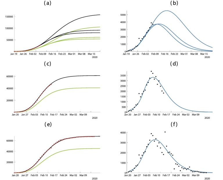
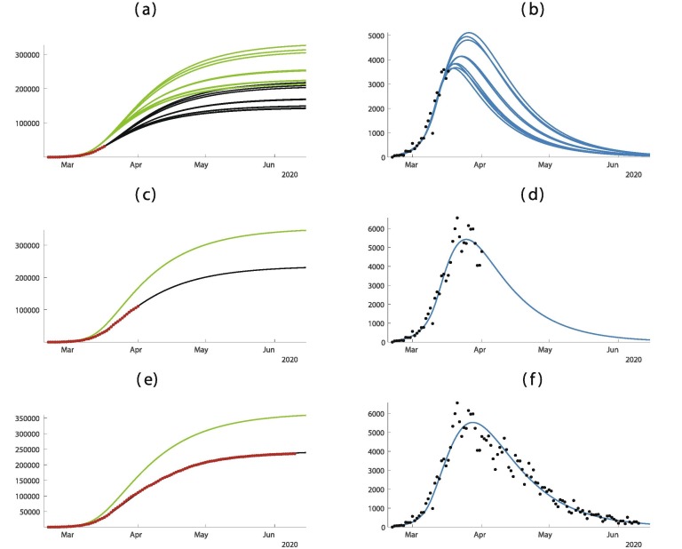
In Fig. 3 , the predictions are improving with time. We observe that if we apply our method too early as in Fig. 3(a) and (b) the predictions vary a lot. But once we pass the turning point as in Fig. 3(c) and (d) the predictions are becoming pretty good and do not vary too much until the end of the epidemic.
Fig. 3.
In this figure we plot the cumulative number of cases of the left hand side and the daily number of cases on the right hand side. In (a) and (b) we use the data until February 5. In (c) and (d) we use the data until February 12. In (e) and (f) we use the data until March 11. The best is obtained for = January = January days, days, and = January 27. The smallest mean absolute deviation is 475.
5.2. Predicting the number of cases for South Korea
The first confirmed case of the pandemic of COVID-19 in South Korea was announced on January 20, 2020. During the following four weeks (January 20 - February 17), South Korea monitored the potential spread of COVID-19 from existing confirmed patients, by using technological resources, such as tracking credit card use and checking CCTV footage of confirmed patients. On February 18, South Korea confirmed its case in Daegu. This patient had continued to go to gatherings of Shincheonji for days after showing symptoms. On February 19, the number of confirmed cases increased by 20 and on February 20 by 70, with a total of 346 confirmed cases by February 21, 2020, according to the Korean Centers for Disease Control (KCDC).
On February 20, the streets of Daegu were empty in reaction to the Shincheonji outbreak. On February 23, the government raised the coronavirus alert to ‘highest level’, and increased testing and contact tracing. Extensive measures were taken to screen the population for the virus, to isolate any infected people, and to quarantine those who were in contact with them. These rapid and extensive measures taken by the South Korean government have been judged successful in limiting the spread of the outbreak, without using the extreme measure of quarantining entire cities.
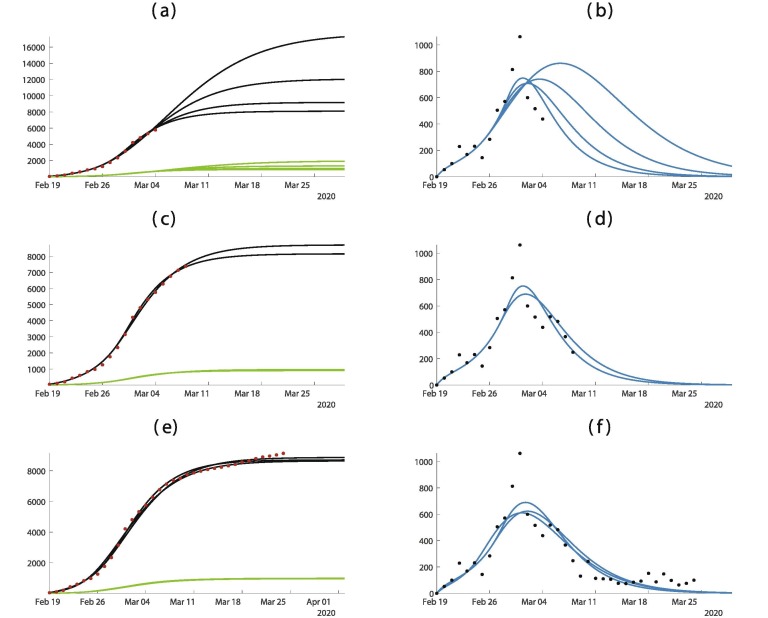
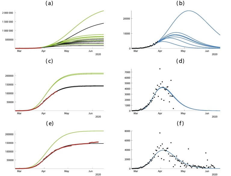
In Fig. 4 , the predictions are improving with time. As in Fig. 3, when we apply our method too early as in Fig. 4(a) and (b) the result is very uncertain.
Fig. 4.
In this figure we plot the cumulative number of cases of the left hand side and the daily number of cases on the right hand side. In (a) and (b) we use the data until March 4. In (c) and (d) we use the data until March 8. (e) and (f) we use the data until March 24. The best is obtained for = February = February days, days, and = February 27. The smallest mean absolute deviation is 144.
5.3. Predicting the number of cases for Italy
On January 31, the first two cases of COVID-19 were confirmed in Rome. On February 22, the government announced a series of isolation measures, such as a new decree imposing the quarantine of more than 50,000 people from 11 different municipalities in Northern Italy. On March 1, nationwide measures began to be implemented. On March 8, Prime Minister Giuseppe Conte extended the quarantine lockdown to cover all the region of Lombardy and 14 other northern provinces. On March 10, Prime Minister Conte increased the quarantine lockdown to cover all of Italy, including travel restrictions, a ban on public gatherings, and a shut down of all commercial and retail businesses except those providing essential services, such as grocery shops and pharmacies. On March 20, the Italian Ministry of Health ordered tighter regulations on free movement. The epidemic in Italy can be divided into the exponential growth phase before February 22. It is reasonable to take N between February 22 and March 10, because the government gradually strengthened control measures to the whole country during the period February 22 to March 10.
5.4. Predicting the number of cases for France
On January 24, the first COVID-19 case was confirmed in Bordeaux, France. The epidemic in France can be divided into the exponential growth phase before March 14. It is reasonable to take N between March 14 and March 17. The reasons are as follows: (1) On March 14, many cultural institutions in the Paris region announced their closure, such as the Louvre, the Eiffel Tower, and institutions in other provinces such as the Chateau de Montsoreau Museum of Contemporary Art; (2) French President Emanuel Macron delivered a speech on March 16, announcing that France entered a “state of war”, and closure measures would be imposed throughout all of France. On March 17, the “ban on foot” was officially launched.
5.5. Predicting the number of cases for Germany
A COVID-19 case was confirmed to have been transmitted to Germany on January 27, 2020. The epidemic in Germany can be divided into the exponential growth phase before March 13. It is reasonable to take N between March 13 and March 15, for the following reasons: (1) On March 13, 14 of the 16 German federal states closed their schools and nurseries; (2) On March 14, several federal states widened their measures to limit public activities. For example, Berlin, Schleswig–Holstein, and Saarland closed bars and other leisure venues. Cologne forbade all public events in the city center.
5.6. Predicting the number of cases for United Kingdom
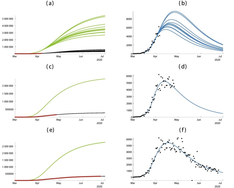
The United Kingdom was slow to implement public distancing measures. On 19 March, the government introduced the Coronavirus Act 2020, which gave discretionary emergency powers in restricting social care facilities, schools, police, the Border Force, local councils, and other public functions. The act went into effect on 25 March 2020. Closures to pubs, restaurants and indoor sports and leisure facilities were imposed by the Health Protection Regulations on March 21. see Fig. 5 .
Fig. 5.
In this figure we plot the cumulative number of cases of the left hand side and the daily number of cases on the right hand side. In (a) and (b) we use the data until March 3. In (c) and (d) we use the data until March 10. (e) and (f) we use the data until March 24. The best is obtained for = February = March days, days, and = March 10. The smallest mean absolute deviation is 1129.
6. Conclusions
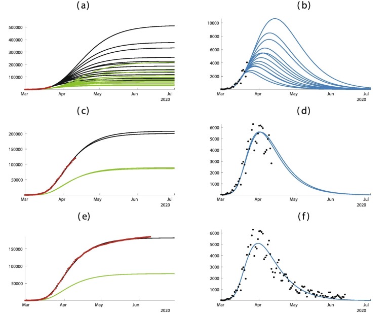
We have applied a method developed in Liu et al., 2020, Liu et al., 2020 to predict the evolution of a COVID-19 epidemic based on reported case data in that region. Our method uses early data, when the epidemic is in its exponential growth phase, corresponding to a constant transmission rate. In Liu et al. (2020) we demonstrated a method to identify this constant transmission rate. When public measures are begun in order to slow down the epidemic, a new phase begins, which we model with a time-dependent exponentially decreasing transmission rate in Liu et al. (2020). In Liu et al. (2020) we applied this method to mainland China, and demonstrated the ability of our model to predict the forward time-line of the epidemic. In Fig. 4 in Liu et al. (2020), we showed how the prediction unfolded week by week, with increasing agreement with reported case data, in mainland China (See Fig. 6 ).
Fig. 6.
In this figure we plot the cumulative number of cases of the left hand side and the daily number of cases on the right hand side. In (a) and (b) we use the data until March 17. In (c) and (d) we use the data until April 1. (e) and (f) we use the data until June 10. The best is obtained for = March = March days, days, and = March 15. The smallest mean absolute deviation is 2347.
In Table 2 we summarized the parameters giving the best fit to the data (See Fig. 7 ).
Table 2.
The parameters are estimated by using the data to fit to the cumulative reported cases data ( is chosen to minimize the error of the fit). For each country the best fit of the data over the all period is obtained by choosing: (1) = January 27 and = January 30 for mainland China; (2) = February 19 and = February 24 for South Korea; (3) = February 23 and = March 10 for Italy; (4) = March 1 and = March 20 for France; (5) = February 24 and = March 11 for Germany; (6) = March 4 and = March 26 for United Kingdom. The parameters and . The values of are obtained by using (3.7), (3.8), (3.4).
| Country | N | |||||||
|---|---|---|---|---|---|---|---|---|
| China | Jan. 20 | Jan. 27 | ||||||
| South Korea | Feb. 19 | Feb. 27 | ||||||
| Italy | Feb. 23 | Mar. 10 | ||||||
| France | March 1 | Mar. 15 | ||||||
| Germany | Feb. 24 | Mar. 13 | ||||||
| United Kingdom | Mar. 4 | Mar. 22 |
Fig. 7.
In this figure we plot the cumulative number of cases of the left hand side and the daily number of cases on the right hand side. In (a) and (b) we use the data until March 22. In (c) and (d) we use the data until April 11. (e) and (f) we use the data until June 10. The best is obtained for = February = March days, days, and = March 13. The smallest mean absolute deviation is 1368.
In this work we use data for the cumulative number of reported cases and the daily number of reported cases for China, South Korea, Italy, France, Germany, and the United Kingdom. With this data, we project the future number of cases, both reported and unreported, in each country. For each country we observe that before the turning point the prediction is very uncertain and several of parameter values of f may fit very well the data before the turning point. However, if we use enough reported case data, such as data up to the turning point, the prediction is pretty good and certain until the end of the epidemic (See Fig. 8 ).
Fig. 8.
In this figure we plot the cumulative number of cases of the left hand side and the daily number of cases on the right hand side. In (a) and (b) we use the data until April 6. In (c) and (d) we use the data until April 26. (e) and (f) we use the data until June 25. The best is obtained for = March = March days, days, and = March 22. The smallest mean absolute deviation is 1248.
A major difficulty for the predictions from the reported cases data, is to determine the date intervals of exponential growth phase. From the Fig. 2(a) this period is clear for mainland China (Jan 19–27). But it is much more difficult to decide for South-Korea (see Fig. 2(a)). By applying our method to the data for South Korea, we find the interval going from February 19 to February 24. This is because the measures imposed for contact tracing and social distancing were very strong. For Italy, the interval is difficult to ascertain (see Fig. 2(c)). We choose February 23 to March 10, but these values may change as more data of reported cases becomes available. For France, Germany, and the United Kingdom, the interval are also difficult to know with present data. Again, future reported case data, will clarify these intervals.
In the case of South Korea, the peak of the epidemic occurred approximately on February 29. In Fig. 4, we see that our model agrees very well the data for South Korea. Accordingly to our model, the daily number of cases reaches a maximum of approximately 700 cases near the turning point February 29. Compared to South Korea, the public interventions in Italy, France, and Germany were relatively late. The peak of the epidemic occurs in Italy around March 14, and the peak of the maximum daily number of cases in our simulation is approximately , which agrees well with the daily reported cases data for Italy. For France, Germany, and the United Kingdom, the number of daily reported cases may still be rising. Our simulations captures these increasing values for exponential growth phase, but the advance to the next phase for both countries requires advanced data.
In general, the dates for the exponential growth interval, and the date N for the start of the new phase after the exponential growth interval, are key elements of our model, and they depend strongly on the implementation of social distancing measures. If these measures are implemented gradually, then the difficulty is increased. In future work we will allow for a series of N and values to account for a more complex implementation of measures that use a time-dependent transmission function depending on these values.
Another difficulty in applying our model is the assumption of the fraction f of total cases reported. The value of f is unknown, but we vary f between to . In future work, we will allow a time-dependent value for f, because in many applications the fraction of reported cases changes over the course of the epidemic. Our model incorporates social distancing measures through the time dependent transmission rate . It is evident that these measures should start as early as possible, and should be as strong as possible. The consequences of late public interventions may have severe consequences for the epidemic outcome. In future work we will apply our methods to other countries and regions within countries in an effort to better understand the evolution of COVID-19 epidemics. In Cotta et al., 2020, Roques et al., 2020 Bayesian’s method has been used successfully. Such a method could be used here as well, and that is left for future work.
In Table 3 we summarized the parameters giving the best fit to the data.
Table 3.
In this table, we summarize the values for (mean duration in days of the asymptomatic phase before symptoms onset), (mean duration in days of the symptomatic phase), and f (the fraction of reported) obtained for the best fits to the cumulative reported data.
| Country | f | ||
|---|---|---|---|
| China | 5 days | 6 days | |
| South Korea | 4 days | 16 days | |
| Italy | 23 days | 14 days | |
| France | 6 days | 15 days | |
| Germany | 15 days | 14 days | |
| United Kingdom | 30 days | 31 days |
The values of (mean duration in days of the asymptomatic phase before symptoms onset) and (mean duration in days of the symptomatic phase) are very uncertain. Reported values have a wide range of variability. In an early report, a value of the asymptomatic phase was given as 5 days in Gandhi et al. (2020). WHO reported that the asymptomatic period is on average 5–6 days, but can be up to 14 days WHO (2020). In recent reports, patients were reported asymptomatic 4–17 days after admission to hospitals (Long et al., 2020), and 9.5 days (Hu et al., 2020). The Centers for Disease Control reported an average value of 6 days for asymptomatic transmission (Centers for Disease Control, 2020). The period of median viral shredding was reported as 19 days pre-symptomatic patients and 14 days for symptomatic patients (Long et al., 2020), and 22.6 days in pre-symptomatic patients and 25.2 days in symptomatic patients (Noh et al., 2020), although viral shedding does not necessarily correlate to infectiousness.
In this work many questions need future considerations. First the data are questionable and may induce a bias in the estimation of parameters. Probably the most significant effect on the data is induced by the daily fluctuations of the number of tests. Such a large fluctuation has been observed in China and other countries when the medical doctors were trying to adapt the number of tests to the number of symptomatic patients. Such a phenomenon may induce a large variation in the number of reported cases. In order to improve our understanding of the real situation from the cumulative reported cases, we can improve the model in several ways. For example we can introduce age groups (see Prem et al., 2020, Griette et al., 2020) or we may examine big cities and their interconnections (see Wu et al., 2020). The method used to fit the data in the present paper has been extended and used successfully for age groups in Japan (Griette et al., 2020). Such a method is general and may probably be applied to other situations (patch models etc …). In future work, we can also incorporate the number of tests (see Roques et al., 2020) which may significantly improve our understanding of COVID-19 epidemics.
Funding
This research was funded by the National Natural Science Foundation of China (Grant No.: 11871007 (ZL)), NSFC and CNRS (Grant No.: 11811530272 (ZL, PM)) and the Fundamental Research Funds for the Central Universities (ZL). This research was funded by the Agence Nationale de la Recherche in France (Project name: MPCUII (PM)).
Conflicts of Interest
Declare conflicts of interest or state “The authors declare no conflict of interest.”
References
- Ahmed I. Analysis of Caputo fractional-order model for COVID-19 with lockdown. Adv. Differ. Eqs. 2020;394 doi: 10.1186/s13662-020-02853-0. [DOI] [PMC free article] [PubMed] [Google Scholar]
- Centers for Disease Control, COVID-19 Pandemic Planning Scenarios, July 10, 2020.https://www.cdc.gov/coronavirus/2019-ncov/hcp/planning-scenarios.html.
- Chowell G., Viboud C. Is it growing exponentially fast? Impact of assuming exponential growth for characterizing and forecasting epidemics with initial near-exponential growth dynamics. Infect. Dis. Model. 2016;1:71–78. doi: 10.1016/j.idm.2016.07.004. [DOI] [PMC free article] [PubMed] [Google Scholar]
- Cotta R.M., Naveira-Cotta C.P., Magal P. Mathematical parameters of the COVID-19 epidemic in Brazil and evaluation of the impact of different public health measures. Biology. 2020;9(8):220. doi: 10.3390/biology9080220. [DOI] [PMC free article] [PubMed] [Google Scholar]
- Gandhi M., Yokoe D.S., Havlir D.V. Asymptomatic transmission, the Achilles’ heel of current strategies to control, COVID-19. N. Engl. J. Med. 2020;382:2158–2160. doi: 10.1056/NEJMe2009758. [DOI] [PMC free article] [PubMed] [Google Scholar]
- Griette Q., Magal P., Seydi O. Unreported cases for Age Dependent COVID-19 Outbreak in Japan. Biology. 2020;9:132. doi: 10.3390/biology9060132. [DOI] [PMC free article] [PubMed] [Google Scholar]
- Guan, W., et al., Clinical characteristics of coronavirus disease 2019 in China. New Engl. J. Med.https://doi.org/10.1056/NEJMc2001468(2020). [DOI] [PMC free article] [PubMed]
- Hu, Z., Song, C., Xu, C., et al., 2020. Clinical characteristics of 24 asymptomatic infections with COVID-19 screened among close contacts in Nanjing, China. Sci. China Life Sci. 63, 706D711.https://doi.org/10.1007/s11427-020-1661-1664. [DOI] [PMC free article] [PubMed]
- Jajarmi A. A new fractional HRSV model and its optimal control: a non-singular operator approach. Phys. A. 2020;547 [Google Scholar]
- Kucharski, A., Russell, T.W., Diamond, C., et al., 2020. Early dynamics of transmission and control of COVID-19: a mathematical modelling study. Lancet. [DOI] [PMC free article] [PubMed]
- Liu Z., Magal P., Seydi O., Webb G. Understanding unreported cases in the 2019-nCov epidemic outbreak in Wuhan, China, and the importance of major public health interventions. MPDI Biol. 2020;9(3):50. doi: 10.3390/biology9030050. [DOI] [PMC free article] [PubMed] [Google Scholar]
- Z. Liu, P. Magal, O. Seydi, and G. Webb, Predicting the cumulative number of cases for the COVID-19 epidemic in China from early data, Mathematical Biosciences and Engineering (to appear). [DOI] [PubMed]
- Liu, Z., Magal, P., Seydi, O., Webb, G. A COVID-19 epidemic model with latency period, Infectious Disease Modelling (to appear). [DOI] [PMC free article] [PubMed]
- Long, Q.-X., Tang, X.-J., Shi, Q.-L., et al., 2020. Clinical and immunological assessment of asymptomatic SARS-CoV-2 infections. Nat. Med. [DOI] [PubMed]
- K. Mizumoto, K. Kagaya, A. Zarebski, and G. Chowell, Estimating the asymptomatic proportion of coronavirus disease 2019 (COVID-19) cases on board the Diamond Princess cruise ship, Yokohama, Japan, 2020. Euro Surveill. 25(10):pii=2000180. doi: 10.2807/1560-7917(2020). [DOI] [PMC free article] [PubMed]
- Mustapha U. Fractional modeling for the spread of Hookworm infection under Caputo operator. Chaos Solitons Fractals. 2020;137 [Google Scholar]
- Nishiura, H., et al., 2020. Estimation of the asymptomatic ratio of novel coronavirus infections (COVID-19). Int. J. Infect. Dis.https://doi.org/10.1016/j.ijid.2020.03.020. [DOI] [PMC free article] [PubMed]
- Noh, J.Y., Yung, J.G., Seong, H., et al., 2020. Asymptomatic infection and atypical manifestations of COVID-19: Comparison of viral shedding duration. J. Infect.https://doi.org/10.1016/j.jinf.2020.05.035. [DOI] [PMC free article] [PubMed]
- Prem K., Liu Y., Russell T.W., Kucharski A.J., Eggo R.M., Davies N., Flasche S., Clifford S., Pearson C.A.B., Munday J.D. The effect of control strategies to reduce social mixing onoutcomes of the COVID-19 epidemic in Wuhan, China: a modelling study. Lancet Public Health. 2020:5. doi: 10.1016/S2468-2667(20)30073-6. [DOI] [PMC free article] [PubMed] [Google Scholar]
- Qiu, J. Covert coronavirus infections could be seeding new outbreaks. Nature. URL: https://www.nature.com/articles/d41586-020-00822-x. [DOI] [PubMed]
- Roda W.C., Varughese M.B., Han D., Li M.Y. Why is it difficult to accurately predict the COVID-19 epidemic? Infect. Disease Model. 2020;5:271–281. doi: 10.1016/j.idm.2020.03.001. [DOI] [PMC free article] [PubMed] [Google Scholar]
- Roques L., Klein E.K., Papaïx J., Sar A., Soubeyrand S. Using early data to estimate the actual infection fatality ratio from COVID-19 in France. Biology. 2020;9(5):97. doi: 10.3390/biology9050097. [DOI] [PMC free article] [PubMed] [Google Scholar]
- Rothe, C., et al., 2020. Transmission of 2019-nCoV infection from an asymptomatic contact in Germany. New Engl. J. Med.https://doi.org/10.1056/NEJMc2001468. [DOI] [PMC free article] [PubMed]
- URL: https://en.wikipedia.org/wiki/2020_coronavirus_outbreak_in_South_Korea.
- URL: https://en.wikipedia.org/wiki/COVID-19_pandemic_in_mainland_China.
- URL: https://en.wikipedia.org/wiki/2020_coronavirus_outbreak_in_Italy.
- URL: https://en.wikipedia.org/wiki/2020_coronavirus_outbreak_in_France.
- URL: https://en.wikipedia.org/wiki/2020_coronavirus_outbreak_in_Germany.
- URL: https://en.wikipedia.org/wiki/COVID-19_pandemic__the_United_Kingdom.
- Verity R., Odell L.C., Dorigatti I. Estimates of the severity of COVID-19 disease. medRxiv. 2020 [Google Scholar]
- Wang, C., et al., 2020. Evolving Epidemiology and Impact of Non-pharmaceutical Interventions on the Outbreak of Coronavirus Disease 2019 in Wuhan, China, Preprint at medRxiv.https://doi.org/10.1101/2020.03.03.20030593.
- WHO, 2020. Coronavirus disease 2019 (COVID-19), Situation Report – 73.
- Wölfel, R., et al., 2020. Virological assessment of hospitalized patients with COVID-2019. Nature.https://doi.org/10.1038/s41586-020-2196-x. [DOI] [PubMed]
- Wu J.T., Leung K., Leung G.M. Nowcasting and forecasting the potential domestic and international spread of the COVID-19 outbreak originating in Wuhan, China: a modelling study. Lancet. 2020 doi: 10.1016/S0140-6736(20)30260-9. [DOI] [PMC free article] [PubMed] [Google Scholar]


