Updated Global Warming Potentials and Radiative Efficiencies of Halocarbons and Other Weak Atmospheric Absorbers

Abstract

Human activity has led to increased atmospheric concentrations of many gases, including halocarbons, and may lead to emissions of many more gases. Many of these gases are, on a per molecule basis, powerful greenhouse gases, although at present‐day concentrations their climate effect is in the so‐called weak limit (i.e., their effect scales linearly with concentration). We published a comprehensive review of the radiative efficiencies (RE) and global warming potentials (GWP) for around 200 such compounds in 2013 (Hodnebrog et al., 2013, https://doi.org/10.1002/rog.20013). Here we present updated RE and GWP values for compounds where experimental infrared absorption spectra are available. Updated numbers are based on a revised “Pinnock curve”, which gives RE as a function of wave number, and now also accounts for stratospheric temperature adjustment (Shine & Myhre, 2020, https://doi.org/10.1029/2019MS001951). Further updates include the implementation of around 500 absorption spectra additional to those in the 2013 review and new atmospheric lifetimes from the literature (mainly from WMO (2019)). In total, values for 60 of the compounds previously assessed are based on additional absorption spectra, and 42 compounds have REs which differ by >10% from our previous assessment. New RE calculations are presented for more than 400 compounds in addition to the previously assessed compounds, and GWP calculations are presented for a total of around 250 compounds. Present‐day radiative forcing due to halocarbons and other weak absorbers is 0.38 [0.33–0.43] W m⁻², compared to 0.36 [0.32–0.40] W m⁻² in IPCC AR5 (Myhre et al., 2013, https://doi.org/10.1017/CBO9781107415324.018), which is about 18% of the current CO₂ forcing.

Key Points

• Radiative efficiencies are reassessed for more than 600 compounds and global warming potentials calculated for around 250 of these

• Forty‐two compounds have >10% different radiative efficiency compared to a comprehensive review in 2013

• Present‐day radiative forcing due to halocarbons and other weak absorbers is 0.38 [0.33–0.43] W m⁻², which is ~18% of the CO₂ forcing

1. Introduction

Anthropogenic forcing of climate change is one of the most important challenges facing humanity. The largest contributor to radiative forcing of climate change is the increased levels of greenhouse gases such as CO₂, N₂O, CH₄, and halocarbons and related compounds. While many halocarbons, such as chlorofluorocarbons (CFCs), are known for depleting stratospheric ozone (Molina & Rowland, 1974; WMO, 2019), they are also powerful greenhouse gases. Despite the phase‐out of several halocarbons through the Montreal Protocol from 1987 and its amendments and adjustments, halocarbons still make an important contribution to radiative forcing of climate change because many have long atmospheric lifetimes. Furthermore, the concentrations of some replacement compounds, such as hydrochlorofluorocarbons (HCFCs) and hydrofluorocarbons (HFCs), are rising. More specifically, Figure 1 (WMO/GAW, 2019) shows that HCFC‐22 has recently become the second most abundant compound (of the greenhouse gases with only anthropogenic sources) after CFC‐12. HFC‐134a has, in only 20 years, increased from very low abundance to become the fourth most abundant halocarbon. Emissions of HFCs, perfluorocarbons, SF₆, and NF₃ are included in the United Nations Framework Convention on Climate Change (UNFCCC). Controls on emissions of HFCs, in addition to CFCs and HCFCs, are included in the 2016 Kigali Agreement to the Montreal Protocol (see discussion in Kochanov et al., 2019).

Figure 1.

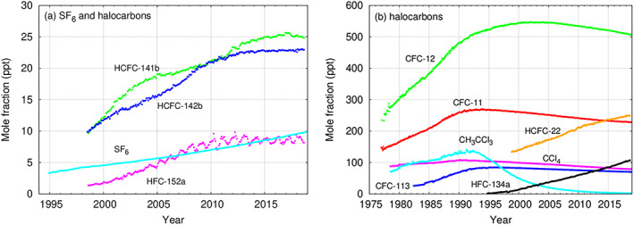
Atmospheric abundances of important halocarbons (and SF₆), separated into (a) lower and (b) higher mole fractions and based on observations from a number of stations (from WMO/GAW, 2019). The plots are based on the data submitted to the World Data Center for Greenhouse Gases supported by the Japan Meteorological Agency by laboratories participating in the GAW program.

Differences in the intensity and wavelength of infrared (IR) absorption bands lead to distinct radiative forcing efficiencies of various gases. Radiative efficiency (RE) is a measure of the radiative forcing for a unit change in the atmospheric concentration of a gas, and for halocarbons and related compounds is usually reported in units of W m⁻² ppb⁻¹. To provide policy makers with guidance on the relative effectiveness of actions limiting the emissions of different gases, metrics have been developed to place the impact of emissions of different gases on a common scale. The most widely used metric is the global warming potential (GWP) with a 100‐year time horizon (hereafter GWP(100)), which is based on the time‐integrated radiative forcing due to a pulse emission of a unit mass of gas, normalized by the reference gas CO₂ and was introduced in the first assessment report of the Intergovernmental Panel on Climate Change (IPCC, 1990) (see section 2.5).

In 2013 we reviewed the literature data and provided a comprehensive and self‐consistent set of new calculations of REs and GWPs for halocarbons and related compounds (Hodnebrog et al., 2013, hereafter referred to as H2013). Unlike the major greenhouse gases, current atmospheric concentrations of these compounds are low enough for the forcing to scale almost linearly with abundance, and we will therefore refer to these compounds as weak atmospheric absorbers. Adopting a common method for calculating REs and GWPs provides a more consistent approach to comparing metrics between different compounds than if these metrics are taken from studies that used different methodologies. Our results were incorporated by the IPCC into the fifth assessment report (AR5) (Myhre et al., 2013) and, as a result, they are now used in national and international agreements. The UNFCCC adopted AR5 values for reporting emissions under the Paris Agreement and the U.S. Environmental Protection Agency (EPA) uses GWP values from AR5 in its reports. To ensure that climate policy decisions are based on the latest scientific data, it is important to periodically review and update the assessments. Additional infrared absorption spectra and refinements in estimations of the atmospheric lifetimes of halocarbons and other compounds have become available since our last review. Specifically, we have considered and included absorption spectra given as supporting information to published papers, and from the HITRAN2016 (Kochanov et al., 2019) and PNNL (Sharpe et al., 2004) databases. Atmospheric lifetimes have recently been updated in WMO (2019) and these estimates have been used here. The provision of GWP(100) values in this paper, and in H2013, should not be seen as an endorsement of that metric, as the choice of metric depends on the policy context (Myhre et al., 2013); the RE and lifetime values presented here can be used to derive values for alternative emission metrics.

We have updated and extended our previous assessment of REs and GWPs for halocarbons and other weak atmospheric absorbers. Updates are based on new absorption spectra for 60 compounds considered in our previous review, the latest estimates of atmospheric lifetimes, and an update to the RE calculation method. The review has been extended to include around 440 additional compounds to bring the total number of compounds considered to more than 600. Included are several isomeric species which have identical empirical formulae but are structurally and spectrally distinct. Therefore, there is no need to consider isomeric compounds together within the context of this review. The radiative forcing contributions of the 40 most abundant halocarbons and related compounds in the atmosphere are estimated. The present work is the most comprehensive review of the radiative efficiencies and GWPs of halogenated compounds performed to date.

2. Data and Method

2.1. Absorption Cross Sections

In addition to the experimental spectra included in H2013 we have included, either in the main or supporting information, all IR absorption spectra available from the HITRAN2016 (Gordon et al., 2017; Kochanov et al., 2019) and PNNL (Sharpe et al., 2004) databases. The vast majority of spectra from PNNL are also available in HITRAN2016 and we have only included data from one of the databases to avoid overlap. The main sources of experimental infrared absorption cross sections in H2013 were the Ford Motor Company (e.g., Sihra et al., 2001), the Spectroscopy and Warming potentials of Atmospheric Greenhouse Gases project (Ballard et al., 2000b; Highwood & Shine, 2000), HITRAN‐2008 (Rothman et al., 2009) and GEISA‐2009 (Jacquinet‐Husson et al., 2011) databases, and data provided by authors of published papers (e.g., Imasu et al., 1995). Several of the spectra used in H2013 were provided in the supporting information and later included in the HITRAN2016 and GEISA‐2015 (Jacquinet‐Husson et al., 2016) databases. Many publications now make available their measured absorption cross sections as supporting information. Since spectra provided as supporting information are typically not in a standardized data format and need to be converted, we could only carry out RE calculations for a limited number of these supporting information spectra, and we have prioritized the 40 most atmospherically abundant compounds. For other studies the reported integrated absorption cross section and RE value, if available, are listed (Tables S1‐S20).

As in H2013, each of the available spectra has been evaluated and if several spectra from the same laboratory group exist, we only use the latest published spectrum. For example, spectra from Sihra et al. (2001) supersede those from Pinnock et al. (1995) and Christidis et al. (1997) due to improvements in the methodology of the Ford laboratory measurements. When more than one spectrum was available from a source, the spectrum that was recorded nearest room temperature and atmospheric pressure was used (see section 2.2 for a discussion of the temperature dependence of cross sections). The choices of spectra to be used in RE calculations have been explained for each group of compounds in the supporting information (Texts S1–S20).

In contrast to H2013, we only consider experimental absorption cross sections that are measured in a laboratory. As a result, 44 of the compounds included in H2013 have been omitted here because experimental spectra are not available, while nine of the compounds that only had calculated spectra in H2013 have been updated with RE values based on experimental spectra. Calculated IR spectra have been published for a vast number of compounds (e.g., Davila et al., 2017; Papanastasiou et al., 2018), with some studies including thousands of compounds (Betowski et al., 2016; Kazakov et al., 2012; McLinden et al., 2014) but these have a considerably larger uncertainty than experimental spectra (see Table 1 of H2013).

2.2. Temperature Dependence of Cross Sections

Although absorption cross sections are temperature dependent, integrated absorption cross sections show little dependence on temperature. The origin of the temperature dependence of absorption cross sections is the strong dependence of rotational states on temperature. Consequently, spectral bands are generally broader and have a lower peak intensity when observed at higher temperatures. This effect is illustrated in Figure 2 for a range of compound types (CFC, halon and sulfur‐containing species), temperature range and pressure. The effect is noticeable even for the 20 K temperature difference illustrated in Figure 2 for CBrClF₂. These small changes in band structure have a negligible effect on calculated REs, and hence GWPs.

Figure 2.

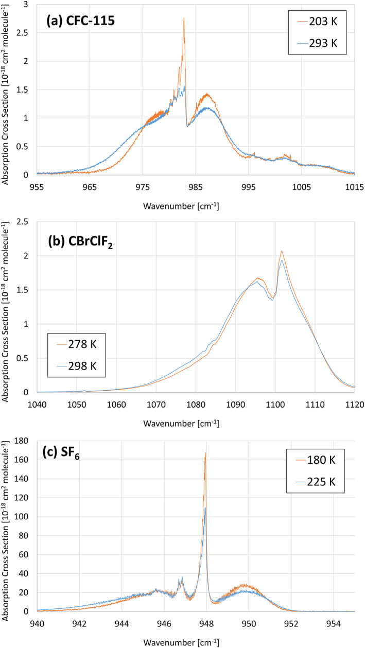
Effect of temperature on band shape. (a) CFC‐115: T = 203 K, p = 0 Torr; T = 298 K, p = 0 Torr (Massie et al., 1991; McDaniel et al., 1991). (b) CBrClF₂: T = 273 K, p = 760 Torr; T = 293 K, p = 760 Torr (Sharpe et al., 2004). (c) SF₆: T = 180 K, p = 75 Torr; T = 225 K, p = 78 Torr (referred to as Varanasi, private communication, 2000, in HITRAN).

However, when molecules exist in two or more distinct conformational forms, the possibility of significant temperature dependence of the integrated cross section exists (Godin et al., 2019). For example, the absorption spectra for CFC‐114 reported by McDaniel et al. (1991) indicate that there are bands within the spectrum that show relatively strong positive temperature dependence, bands that show a weak negative temperature dependence, and bands that are not temperature dependent. These observations can be rationalized in terms of the temperature dependence of the populations of the two different conformers of CFC‐114. However, the integrated cross sections of most molecules show little temperature dependence, and for consistency, we have used spectra obtained at ambient temperatures, where the experimental uncertainties are typically smallest.

2.3. Radiative Efficiency

In H2013, a common method was used to calculate the RE for most gases. This employed the “Pinnock curve” (Pinnock et al., 1995) where the RE as a function of wave number was calculated for a weak absorber absorbing equally at all wave numbers. Multiplying this curve by the absorption cross section of a given gas yields its RE. In H2013 the Pinnock curve was updated (Figure 3, blue line), most notably by increasing its spectral resolution from 10 to 1 cm⁻¹ using the Oslo Line‐By‐Line (OLBL) radiative transfer model run at 0.02 cm⁻¹ resolution (note that there was a typo in the caption of Figure 6 in H2013, wrongly stating a resolution of 0.2 cm⁻¹); the updated calculations also used more refined atmospheric profiles of temperature, cloudiness and greenhouse gas concentrations. For instance, the atmospheric representation was expanded from one global mean profile to two profiles, one for the tropics and one for the extratropics, and the inclusion of refined cloud profiles led to weaker RE in the 800–1,200 cm⁻¹ region (see sections 2.3 and 3.3.1 of H2013 for details). The Pinnock et al. (1995) method, and the H2013 update, yield the instantaneous RE (i.e., the radiative efficiency in the absence of stratospheric temperature adjustment). Since the RE, which includes this adjustment, provides a more accurate representation of a gas's impact on surface temperature, H2013 incorporated a correction to account for this. For most gases, the instantaneous RE was simply increased by 10%. For several gases (CFC‐11, CFC‐12, HFC‐41, and PFC‐14) the correction was explicitly calculated using OLBL, either because of the absolute importance of that gas or because, in the case of HFC‐41, it was known that the RE is less than its instantaneous value. However, this approach was somewhat ad hoc and may not have been applicable to all gases.

Figure 3.

Instantaneous radiative forcing (IRF) efficiency (for a 0–1 ppb increase in mixing ratio) per unit cross section compared between the previous (Hodnebrog et al., 2013) and updated (Shine & Myhre, 2020) results from the Oslo line‐by‐line (OLBL) radiative transfer model run at 0.02 cm⁻¹ spectral resolution. Also shown is the new radiative forcing (RF) efficiency where the effect of stratospheric temperature adjustment per unit cross section, based on 10 cm⁻¹ narrow band model (NBM) simulations (Shine & Myhre, 2020), have been used to modify the OLBL curve. The curves have been averaged to 10 cm⁻¹ spectral resolution in the plot, to improve readability, but RE calculations in this paper have been made using a 1 cm⁻¹ version of the RF efficiency curve (as provided in the supporting information of Shine and Myhre, 2020).

Shine and Myhre (2020) have incorporated stratospheric temperature adjustment into the Pinnock curve for the first time, by calculating the impact of absorption by a gas at a given wave number on stratospheric temperatures (Figure 3, red vs. purple line). The calculation of this adjustment is computationally intensive, as the RE due to absorption by a gas at a given wave number occurs not only at that wave number (as in the case of instantaneous RE) but now depends on the emission by gases (mostly CO₂, H₂O, and O₃) at all other wave numbers. Because of this, Shine and Myhre (2020) calculated the effect of adjustment using a narrow‐band (10 cm⁻¹) radiation code, and applied this to updated instantaneous RE calculations using OLBL (which included an improved representation of the water vapor continuum and some changes to the representation of clouds). The new method reproduced detailed calculations for a range of gases (including HFC‐41 and CFC‐11) to better than 1.5%. Although more complicated in its derivation, it is no more complicated than the original Pinnock method in its application. This new method (which also requires the use of the lifetime correction described in section 2.4) is applied to all gases here and hence improves the relative consistency of derived REs.

2.4. Atmospheric Lifetimes and Lifetime Correction

The atmospheric lifetime of a compound is required for calculations of GWPs and Global Temperature‐change Potentials (GTPs) (see section 2.5). The RE value obtained from the method described in section 2.3 assumes the compound is well‐mixed in the atmosphere. Most of the compounds included in this study have a nonuniform vertical and horizontal distribution in the atmosphere, and the lifetime can be used to correct for that. Here we use the method presented in H2013 (their section 3.3.4), where two approximations are given depending on the primary loss mechanism of the compound. One approximation is used for compounds primarily being lost through photolysis in the stratosphere: the fractional correction f to the RE of f(τ) = 1 − 0.1826τ^−0.3339 is applicable for lifetimes τ of 10 < τ < 10⁴ years. Another approximation is used for compounds primarily lost through reaction with OH in the troposphere: $f\left(\tau \right)=\frac{a{\tau }^b}{1+c{\tau }^d}$, where a = 2.962, b = 0.9312, c = 2.994, d = 0.9302, and is applicable for 10⁻⁴ < τ < 10⁴ years. The lifetime corrections for very short‐lived compounds should be treated as particularly approximate, as the correction depends on where the emissions take place. Excepted from these approximations are CFC‐11, CFC‐12, and Halon‐1211 because explicit LBL calculations were made in H2013 (see their section 3.3.3) to derive factors to account for non‐uniform mixing. The derived factors were 0.927, 0.970, and 0.937, respectively, and are used here in the RE calculations for these compounds. These factors are less than one, despite being quite long‐lived compounds, because of stratospheric loss due to photolysis.

The recent WMO (2019) report gives the most up‐to‐date and complete overview of atmospheric lifetimes of halocarbons and related compounds, and we rely on these estimates. Explanations and sources for the lifetime estimates in WMO (2019) are given for each compound in their Chapter 1.2 and Table A‐1. For some compounds that do not have a lifetime estimate in WMO (2019), lifetime estimates have been taken from previous literature and sometimes as an average across different estimates if more studies exist (see Tables S1–S20 for references to lifetime estimates). For several compounds, we are not aware of any estimates of lifetimes; for these we only present REs assuming a constant horizontal and vertical distribution in the atmosphere, and no estimates of GWPs can be given.

2.5. Description of Metrics

The most widely used emission metric in climate policy is the GWP. It was introduced by IPCC (1990) where values for three time horizons (20, 100, and 500 years) were given. The GWP values were updated in following assessment reports. GWP has been widely adopted in climate policies, and the Kyoto Protocol adopted GWPs for a time horizon of 100 years as its metric for implementing a multigas approach. At UNFCCC COP24 it was decided to use GWP(100) for reporting national emissions to the Paris Agreement, while parties may in addition use other metrics (e.g., global temperature change potential) to report supporting information on aggregate emissions and removals of greenhouse gases, expressed in CO₂ equivalents (UNFCCC, 2019).

The GWP is based on the time‐integrated radiative forcing due to a pulse emission of a unit mass of a gas. It can be given as an absolute GWP for gas i (AGWP_i) (usually in W m⁻² kg⁻¹ year) or as a dimensionless value by dividing the AGWP_i by the AGWP of a reference gas, normally CO₂. Thus, the GWP for gas i over a time horizon of H years is defined as

$${\mathit{GWP}}_i\left(H\right)=\frac{{\int }_0^H{\mathit{RF}}_i\left(t\right)\mathrm{d}t}{{\int }_0^H{\mathit{RF}}_{{\mathit{CO}}_2}\left(t\right)\mathrm{d}t}=\frac{{\mathit{\text{AGWP}}}_i\left(H\right)}{{\mathit{\text{AGWP}}}_{{\mathit{CO}}_2}\left(H\right)}.$$

IPCC has usually presented GWPs for a time horizon (H) of 20, 100, and 500 years (although IPCC AR5 (Myhre et al., 2013) only gave GWPs for 20 and 100 years). We use updated lifetimes and RE values presented in section 3 to calculate GWPs for 20, 100, and 500 years as in H2013.

The models used to calculate the impulse response function for CO₂ (Joos et al., 2013) include climate‐carbon cycle feedbacks, but usually no feedbacks are included for the non‐CO₂ gases when metrics are calculated. IPCC AR5 (Myhre et al., 2013) included this feedback tentatively in the metric values (see their Table 8.7 and supporting information Table 8.SM.16), which increased the GWP(100) values by 10–20%. Gasser et al. (2017) found that accounting for climate‐carbon feedback increases the emission metrics of non‐CO₂ species but, in most cases, less than indicated in AR5. They also found that when the feedback is removed for both the reference and target gas, the relative metric values are generally only modestly different compared to when the feedback is included in both (absolute metric values change more markedly); in the case of GWP(100) the differences are less than 1%. As pointed out by Gasser et al. (2017), including or excluding the climate–carbon feedback ultimately depends on the user's goal, but consistency should be ensured in either case. To resolve the consistency issue, we have excluded the climate‐carbon feedback also for CO₂ by using the impulse response function for CO₂ based on the Gasser et al. (2017) simple Earth system model (see their Appendix C); their model shows very good agreement with Joos et al. (2013) when the climate‐carbon feedback is included. Our documentation of input data and presentation of calculations allow for the inclusion of the climate‐carbon feedback to our results in further studies or applications, both for CO₂ and the non‐CO₂ compounds.

Changes to the parameters in AGWP_CO2 impact all GWP values, and the GWP(100) values presented in section 3 are about 14% higher than if the old AGWP_CO2 from AR5 or H2013 had been used. This is due to two changes: (i) The impulse response function for CO₂ is updated as explained above and (ii) the RE of CO₂ is updated using 409.8 ppm for 2019 (Butler & Montzka, 2020) and the simplified expression for CO₂ RF presented in Etminan et al. (2016), which is an update of the formula from Myhre et al. (1998) used in IPCC assessment reports since TAR (IPCC, 2001). Among other improvements, Etminan et al. (2016) made more extensive use of line‐by‐line calculations compared to Myhre et al. (1998). Using the new formula, a 1 ppm change in the CO₂ concentration at current (year 2019) levels of CO₂ (409.8 ppm) and N₂O (331.9 ppb) (Butler & Montzka, 2020) gives a radiative efficiency for CO₂ of 0.012895 W m⁻² ppm⁻¹. The new AGWP_CO2 values for 20, 100, and 500 year time horizons are 2.290 × 10⁻¹⁴, 8.064 × 10⁻¹⁴, and 2.694 × 10⁻¹³ W m⁻² yr (kgCO₂)⁻¹, respectively. The AGWP_CO2(100) value in AR5 (Myhre et al., 2013) and H2013 was about 14% higher, mainly because we updated the impulse response function (accounts for about 8% of the 14% change) and because of a higher atmospheric concentration of CO₂ which lowers its RE (accounts for ~5%), and slightly because of the new formula from Etminan et al. (2016) (accounts for ~1%). Accounting for all these changes, but including the climate‐carbon feedback for CO₂, as has been done in much of the prior literature, would give AGWP_CO2 values which are 3%, 8%, and 13% higher for 20, 100, and 500 year time horizons, respectively.

It is worth highlighting that the impact of increasing CO₂ mixing ratios on GWP values is the net result of two opposing effects. First, many CO₂ absorption features are saturated, or close to saturation, and hence the RE of CO₂ decreases as its mixing ratio increases. Second, the fraction of CO₂ remaining in the atmosphere (measured by the impulse response function) increases with CO₂ mixing ratio (see Figure 8.31 in Myhre et al., 2013). The first effect decreases AGWP_CO2 while the second effect increases AGWP_CO2. Hence, GWP calculations for optically thin gases which are defined as AGWP_X/AGWP_CO2 will change with CO₂ mixing ratio.

An alternative, the GTP was introduced by Shine et al. (2005). It uses the change in global mean temperature following a pulse emission for a chosen point in time as the impact parameter. While GWP is a metric integrated over time, the GTP is based on the temperature change per unit emissions for a selected year, t after the pulse emission. As for the GWP, the impact of CO₂ is normally used as reference:

$$\mathit{GTP}{\left(t\right)}_i=\mathit{\text{AGTP}}{\left(t\right)}_i/\mathit{\text{AGTP}}{\left(t\right)}_{{\mathit{CO}}_2}=\mathrm{\Delta }T{\left(t\right)}_i/\mathrm{\Delta }T{\left(t\right)}_{\mathit{CO}2},$$

where AGTP (K kg⁻¹) is the absolute GTP. The GTP uses the same input as for GWP but in addition includes a temperature response function that represents the thermal inertia of the climate system. AR5 presented values for both GWP and GTP. Here we follow the method used by AR5 (Myhre et al., 2013) and H2013 for calculating GTPs, except that the impulse response function and RE for CO₂ are updated as explained above and the climate response parameters are updated from Boucher and Reddy (2008) to Geoffroy et al. (2013) (as given in Appendix C of Gasser et al., 2017), which are based on an ensemble of models from the Coupled Model Intercomparison Project phase 5 (CMIP5) (Taylor et al., 2011) and involve a lower climate sensitivity (0.88 compared to 1.1 K (W m⁻²)⁻¹ in Boucher and Reddy, 2008). The new AGTP_CO2 values for 20, 50, and 100 year time horizons are 5.413 × 10⁻¹⁶, 4.559 × 10⁻¹⁶, and 4.146 × 10⁻¹⁶ K (kgCO₂)⁻¹, respectively. Including the climate‐carbon feedback for CO₂, but keeping all other parameters the same, would give AGTP_CO2 values which are 5%, 8%, and 11% higher, respectively.

There continues to be a vigorous debate about the applicability of different emission metrics (e.g., Myhre et al., 2013); metric choice depends on the particular policy context in which they are applied, and the degree to which continuity of choice is important in that context (e.g., Allen et al., 2018; Cain et al., 2019; Rogelj & Schleussner, 2019). A specific development has been the suggested use of metrics that compare one‐off pulse emissions of long‐lived gases (such as CO₂) with step‐changes in emissions of short‐lived species (e.g., gases with lifetimes less than a few decades), on the basis that this leads to a more informed comparison of their ultimate impact on temperature; such approaches can either adopt GWP values, but adapt their usage (Allen et al., 2016) or more directly compute the pulse‐step equivalence (W. J. Collins et al., 2019). In the context of this review, the important point is that all such metrics require the same set of inputs (RE and lifetimes).

It is important to note that the RE and GWP(100) calculations presented here only include the direct effect, while indirect effects can be important for several compounds. Some compounds, and particularly CFCs and halons, influence radiative forcing indirectly through depletion of stratospheric ozone as shown in other work (e.g., Daniel et al., 1995; WMO, 2019). The removal of organic compounds by reaction with OH in the troposphere acts as a source of ozone and prolongs the lifetime of methane, and this has been shown to be important for several hydrocarbons (W. J. Collins et al., 2002; Hodnebrog et al., 2018).

2.6. Uncertainties

An overview of estimated contributions to uncertainties associated with the radiative forcing of halocarbons was given in Table 1 of H2013. A total RE uncertainty of ~13% was estimated for compounds with lifetimes longer than about 5 years, and ~23% for compounds with lifetimes shorter than that. The much higher uncertainty for shorter‐lived compounds is caused by the difficulty of estimating nonuniform horizontal and vertical distributions in the atmosphere, which in turn are dependent on the location of emissions (see section 2.4).

Table 1 gives updated estimates of contributions to the total radiative forcing uncertainties. As in H2013, the uncertainty estimates are based on published literature and subjective judgment and we estimate the total uncertainty to be valid for a 5% to 95% (90%) confidence range. The total RF uncertainty, calculated using the root‐sum‐square (RSS) method, is ~14% and 24% for compounds with lifetimes longer and shorter than ~5 years, respectively. These total RF uncertainties are slightly higher than in H2013 and explanations are given below.

Table 1.

Estimated Contributions to the Total Radiative Forcing Uncertainty

Source of uncertainty	Estimated contribution to total RF uncertainty	References used as basis for uncertainty estimates
Experimental absorption cross‐sections	~5%	Ballard et al. (2000a),Bravo et al. (2010), and Forster et al. (2005)
‐neglected far infrared bands	~3%
‐neglected shortwave bands	~5%
Radiation scheme	~5%	W. D. Collins et al. (2006), Forster et al. (2005), and Oreopoulos et al. (2012)
Clouds	~5%	Forster et al. (2005) and Gohar et al. (2004)
Spectral overlap and water vapor distribution	~3%	Forster et al. (2005), Jain et al. (2000), and Pinnock et al. (1995)
Surface emissivity and temperature, and atmospheric temperature	~5%	Forster et al. (2005)
Tropopause level	~5%	Forster et al. (2005),Freckleton et al. (1998), and Myhre and Stordal (1997)
Temporal and spatial averaging	~1%	Freckleton et al., 1998, and Myhre and Stordal (1997)
Stratospheric temperature adjustment	~2%	Forster et al. (2005), Gohar et al. (2004), and Shine and Myhre (2020)
Nonuniform vertical profile	~5% for lifetimes > ~5 years,	Hodnebrog et al. (2013) and Sihra et al. (2001)
	~20% for lifetimes < ~5 years
Total (RSS)	~14% for lifetimes > ~5 years
	~24% for lifetimes < ~5 years

One issue with the use of laboratory data is that it does not always cover the entire spectral range for which radiative forcing is important (see, e.g., Figure 3). For example, the PNNL measurements mostly cover the 600–6,500 cm⁻¹ wave number range, and so their use would neglect any absorption (and hence forcing) at lower wave numbers, although in general it extends to much higher wave numbers than those in other data sets.

The uncertainty due to lack of spectral data at low wave numbers cannot be assessed for every gas in our analysis, but there is some evidence to indicate its typical size. Highwood and Shine (2000) computed the contribution of wave numbers less than 700 cm⁻¹ to the RE for HFC‐134a and found it contributed around 2% to the forcing. Bravo et al. (2010) presented an analysis of the RE due to a set of seven perfluorocarbons. They compared the RE calculated using ab initio methods for the wave number interval 0–2,500 cm⁻¹ with calculations for the wave number interval 700–1,400 cm⁻¹, chosen because it coincided with the wave number range for their associated laboratory measurements. Most of the additional absorption was at wave numbers below 700 cm⁻¹. They found that the integrated absorption cross sections and REs for the narrow range were within 2% for the lighter PFCs, but this difference increased to 10% for heavier PFCs. Since many of the measured data sets (e.g., the PNNL data) use a broader wavelength range than 700–1,400 cm⁻¹, it is unlikely that our estimates are systematically in error by such a large amount. Nevertheless, we introduce an additional generic uncertainty to our estimates, which was not included in the analysis of H2013, of ~3% due to neglected bands (Table 1); clearly this could be systematically investigated in future work, perhaps by including ab initio calculations outside the range of measured cross sections.

Another source of uncertainty not considered in H2013 is the contribution to RE from absorption of shortwave (SW), or solar, radiation in the near‐infrared (3,000 to 14,000 cm⁻¹). There has been renewed interest in the SW forcing due to methane (e.g., W. D. Collins et al., 2018; Etminan et al., 2016). Etminan et al. (2016) find the direct effect of methane's near‐IR bands enhances its forcing by 6% but there is an additional 9% impact via the effect of this absorption on stratospheric temperatures (and hence on longwave forcing). This contrasts with the impact of the near‐IR bands of CO₂ which cause a decrease of a few percent, because much of the additional forcing is at higher altitudes. The contribution of these near‐IR bands to RE is further complicated by the fact that it depends strongly on the overlap between these bands and those of water vapor (Etminan et al., 2016), many of which are saturated for typical atmospheric paths, making generic statements difficult.

The potential impact of SW absorption is difficult to constrain for the diverse range of gases discussed here, without much more detailed study, not least because many of the experimental data sets do not extend to such high wave numbers (the PNNL data are a notable exception). For the heavier halogenated gases, the strongest fundamental and combination bands will generally be at lower wave numbers, at which SW absorption is less important (see, e.g., Bera et al., 2009). The lighter, more hydrogenated, gases, will have more significant absorption bands in the solar near‐infrared but, on the other hand, these gases are likely to be much shorter‐lived, so that their impact on stratospheric temperatures is likely to be lower. We introduce an additional uncertainty of ~5% due to the potential effect of this shortwave absorption (Table 1).

Since H2013, surface emissivity has been included as a source of uncertainty together with surface temperature and atmospheric temperature, and consequently the estimated contribution to RF uncertainty has been increased from ~3% to ~5% (Table 1). The stratospheric temperature adjustment is now based on a much more sophisticated method compared to the generic 10% increase used in H2013 (see section 2.3), and we have lowered the uncertainty contribution for this term from ~4% to ~2%. The remaining sources of uncertainties and their estimated contributions given in Table 1 are unchanged, and we refer to H2013 for detailed explanations of each term.

Uncertainties in the atmospheric lifetime of the compounds are also important for metric calculations, and since H2013, SPARC (2013) have provided recommended lifetime values and uncertainties for a range of halocarbons. Their estimates are derived using atmospheric chemistry transport and inverse modeling, and analysis of atmospheric observations and laboratory measurements. Possible uncertainty ranges for most of the compounds in SPARC (2013) have been evaluated in Velders and Daniel (2014; their Table 1) and range from ±3% to ±33% (1 standard deviation), depending on the compound; they are typically in the range from ±15% to ±20% (or ±25% to ±33% when converted from 1 standard deviation to 5–95% (90%) confidence range). However, Velders and Daniel (2014) point out that the possible uncertainty range is likely an overestimation of the true uncertainty and the most likely range, given for some of the compounds, is substantially lower (±12% to ±20% when converted from 1 standard deviation to 5–95% (90%) confidence range).

GWP uncertainties are affected by uncertainties in the compound's lifetime, RE and the AGWP_CO2, and uncertainties in GWP and/or GTP have been investigated in previous studies (Boucher, 2012; Hodnebrog et al., 2013; Olivié & Peters, 2013; Reisinger et al., 2010; Velders & Daniel, 2014; Wuebbles et al., 1995). H2013 (see their section 3.6.4) estimated GWP(100) uncertainties of ±38% and ±34% (5–95% (90%) confidence) for CFC‐11 and HFC‐134a, respectively. GWP(100) uncertainties for six HFCs in WMO (2015; their Tables 5 and 6) were approximately in the range 30–50%, which is similar to the GWP(100) uncertainties for several ozone‐depleting substances given in Velders and Daniel (2014) (their Table 4). We estimate that the uncertainties given in H2013, WMO (2015) and Velders and Daniel (2014) (approximately in the range 30–50%) are similar for the GWP(100) values calculated here and are probably also representative for most other halocarbons with similar or longer lifetimes.

3. Results and Discussion

3.1. Updated Spectra, REs, and GWPs for the Most Abundant Halocarbons and Related Compounds

This section broadly follows the structure of section 4.1 in H2013, where absorption cross sections and radiative efficiency estimates in the literature were reviewed and new RE and GWP calculations were presented. However, we limit this section to only include studies and spectra that were not included in H2013, and only to the 40 most abundant halocarbons presented in Table 7 of Meinshausen et al. (2017) (see section 3.3 for other compounds). Also, only experimental spectra are used as a basis for our calculations here, unlike H2013 which included RE and GWP calculations for some compounds where only calculated spectra existed. In cases where spectra have been measured at different temperatures, we have used the spectra closest to room temperature (see section 2.2 for a discussion of temperature dependence of cross sections). All REs are given for all‐sky and with stratospheric temperature adjustment included (see section 2.3). The lifetime correction method from H2013, to account for a nonhomogeneous vertical and horizontal distribution in the atmosphere, has been applied to the calculated REs (see section 2.4).

Table 2 lists absorption cross sections that are new since H2013 and Tables S1–S6 in the supporting information list all (to the best of our knowledge) absorption cross sections and reported RE values from the literature. Tables S1–S6 also include calculations using the Pinnock curve from H2013 for easier identification of possible changes in RE that are due to the updated Pinnock curve from Shine and Myhre (2020). We have followed the International Union of Pure and Applied Chemistry, IUPAC, naming scheme and included the unique Chemical Abstract Service Registry Number, CASRN, for each compound listed in the tables. Table 3 presents updated atmospheric lifetimes, REs, and GWP(100) values and discussions of the results are given below for each group of compounds. RE values with more significant figures, needed to reproduce the GWP(100) values, are given in the supporting information.

Table 2.

Integrated Infrared Absorption Cross‐Section Updates (S) Since the H2013 Review for the 40 Most Abundant Halocarbons and Related Compounds in the Atmosphere

Name	CASRN	Identifier	Formula a	T (K)	Wn. range (cm−1)	S b	Reference	Database c	New d
Chlorofluorocarbons
Trichlorofluoromethane	75‐69‐4	CFC‐11	CCl3F	298	570–3,000	10.1	Sharpe et al. ( 2004 )	H16	S
Dichlorodifluoromethane	75‐71‐8	CFC‐12	CCl2F2	294	800–1,270	13.5	Harrison ( 2015a )	H16	S
				296	600–3,000	13.9	Sharpe et al. ( 2004 )	P	S
1,1,2‐Trichloro‐1,2,2‐trifluoroethane	76‐13‐1	CFC‐113	CCl2FCClF2	298	620–3,000	14.6	Sharpe et al. ( 2004 )	H16	S
1,2‐Dichloro‐1,1,2,2‐tetrafluoroethane	76‐14‐2	CFC‐114	CClF2CClF2	298	600–3,000	17.4	Sharpe et al. ( 2004 )	H16	S
1‐Chloro‐1,1,2,2,2‐pentafluoroethane	76‐15‐3	CFC‐115	CClF2CF3	296	946–1,368	11.9	Totterdill et al. ( 2016 )		B
				296	525–3,000	20.1	Sharpe et al. ( 2004 )	P	S
Hydrochlorofluorocarbons
Chlorodifluoromethane	75‐45‐6	HCFC‐22	CHClF2	295	730–1,380	10.5	Harrison ( 2016 )	H16	S
				296	550–3,000	10.8	Sharpe et al. ( 2004 )	P	S
1,1‐Dichloro‐1‐fluoroethane	1717‐00‐6	HCFC‐141b	CH3CCl2F	295	705–1,280		Harrison (2019)		L
				283	570–1,470	8.0	Le Bris et al. ( 2012 )		S
				298	550–3,000	8.4	Sharpe et al. ( 2004 )	H16	S
1‐Chloro‐1,1‐difluoroethane	75‐68‐3	HCFC‐142b	CH3CClF2	283	650–1,500	10.7	Le Bris and Strong ( 2010 )	H16	S
				298	600–3,000	11.2	Sharpe et al. ( 2004 )	H16	S
Hydrofluorocarbons
Trifluoromethane	75‐46‐7	HFC‐23	CHF3	294	950–1,500	12.3	Harrison ( 2013 )	H16	S
				296	600–3,000	12.7	Sharpe et al. ( 2004 )	P	S
Difluoromethane	75‐10‐5	HFC‐32	CH2F2	298	510–3,000	7.0	Sharpe et al. ( 2004 )	H16	S
1,1,1,2,2‐Pentafluoroethane	354‐33‐6	HFC‐125	CHF2CF3	298	510–3,000	17.4	Sharpe et al. ( 2004 )	H16	S
1,1,1,2‐Tetrafluoroethane	811‐97‐2	HFC‐134a	CH2FCF3	296	750–1,600	13.2	Harrison (2015b)	H16	S
				296	600–3,000	14.2	Sharpe et al. ( 2004 )	P	S
1,1,1‐Trifluoroethane	420‐46‐2	HFC‐143a	CH3CF3	296	570–1,500	13.8	Le Bris and Graham ( 2015 )	H16	B
				298	500–3,000	13.9	Sharpe et al. ( 2004 )	H16	S
1,1‐Difluoroethane	75‐37‐6	HFC‐152a	CH3CHF2	298	525–3,000	8.0	Sharpe et al. ( 2004 )	H16	S
1,1,1,2,3,3,3‐Heptafluoropropane	431‐89‐0	HFC‐227ea	CF3CHFCF3	298	500–3,000	25.3	Sharpe et al. ( 2004 )	H16	S
1,1,1,2,2,3,4,5,5,5‐Decafluoropentane	138495‐42‐8	HFC‐43‐10mee	CF3CHFCHFCF2CF3	305	550–1,600	30.1	Le Bris et al. ( 2018 )		B
				298	500–3,000	30.4	Sharpe et al. ( 2004 )	H16	S
Chlorocarbons and Hydrochlorocarbons
1,1,1‐Trichloroethane	71‐55‐6	Methyl chloroform	CH3CCl3	298	500–3,000	5.3	Sharpe et al. ( 2004 )	H16	S
Tetrachloromethane	56‐23‐5	Carbon tetrachloride	CCl4	296	700–860	6.7	Harrison et al. (2017)	H16	S
				295–8	730–825	6.3	Wallington et al. ( 2016 )		B
				298	730–825	6.4	Sharpe et al. (2004)	P	L
Chloromethane	74‐87‐3	Methyl chloride	CH3Cl	295–8	660–1,620	0.8	Wallington et al. ( 2016 )		B
				296	600–3000	1.3	Sharpe et al. (2004)	P	S
Dichloromethane	75‐09‐2	Methylene chloride	CH2Cl2	295–8	650–1,290	2.6	Wallington et al. ( 2016 )		B
				298	600–3,000	2.8	Sharpe et al. (2004)	H16	S
Trichloromethane	67‐66‐3	Chloroform	CHCl3	295–8	720–1,245	4.4	Wallington et al. ( 2016 )		B
				298	580–3,000	5.0	Sharpe et al. (2004)	H16	S
Bromocarbons, hydrobromocarbons and halons
Bromomethane	74‐83‐9	Methyl bromide	CH3Br	296	550–3,000	1.1	Sharpe et al. ( 2004 )	P	S
Bromochlorodifluoromethane	353‐59‐3	Halon‐1211	CBrClF2	298	600–3,000	13.2	Sharpe et al. ( 2004 )	H16	S
Bromotrifluoromethane	75‐63‐8	Halon‐1301	CBrF3	298	510–3,000	16.1	Sharpe et al. ( 2004 )	H16	S
1,2‐Dibromo‐1,1,2,2‐tetrafluoroethane	124‐73‐2	Halon‐2402	CBrF2CBrF2	298	550–3,000	16.1	Sharpe et al. ( 2004 )	H16	S
Fully fluorinated species
Nitrogen trifluoride	7783‐54‐2		NF3	296	600–1,970	7.3	Totterdill et al. ( 2016 )		B
				298	600–3,000	7.2	Sharpe et al. ( 2004 )	H16	S
Sulfur hexafluoride	2551‐62‐4		SF6	295	650–2,000	24.0	Kovács et al. (2017)		L
				298	560–3,000	21.2	Sharpe et al. ( 2004 )	H16	S
Sulfuryl fluoride	2699‐79‐8		SO2F2	298	500–3,000	14.0	Sharpe et al. ( 2004 )	H16	S
Tetrafluoromethane	75‐73‐0	PFC‐14	CF4	298	570–3,000	19.8	Sharpe et al. ( 2004 )	H16	S
Hexafluoroethane	76‐16‐4	PFC‐116	C2F6	298	500–3,000	23.1	Sharpe et al. ( 2004 )	H16	S
Octafluoropropane	76‐19‐7	PFC‐218	C3F8	298	600–3,000	27.5	Sharpe et al. ( 2004 )	H16	S
Octafluorocyclobutane	115‐25‐3	PFC‐C 318	cyc (‐CF2CF2CF2CF2‐)	298	550–3,000	21.7	Sharpe et al. ( 2004 )	H16	S
Decafluorobutane	355‐25‐9	PFC‐31‐10	n‐C4F10	298	500–3,000	32.4	Sharpe et al. ( 2004 )	H16	S
Dodecafluoropentane	678‐26‐2	PFC‐41‐12	n‐C5F12	278	500–3,000	37.3	Sharpe et al. ( 2004 )	H16	S

Note. Spectra used in the present RE calculations are indicated in bold (see Tables S1–S6 in the supporting information for a complete list of spectra used in RE calculations).

^acyc, cyclic compound.

^bIntegrated absorption cross section given in units of 10⁻¹⁷ cm² molecule⁻¹ cm⁻¹.

^cAbsorption cross section downloaded from database: H16, HITRAN 2016; P, PNNL.

^dNew data since H2013: L, literature; S, spectrum; B, both.

Table 3.

Lifetimes (τ), Radiative Efficiencies and Direct Effect GWPs (Relative to CO₂) for the 40 Most Abundant Halocarbons and Related Compounds in the Atmosphere

			τ (yr)		RE (W m−2 ppb−1)		GWP(100)
Identifier/name	Formula	CASRN	H2013 a	WMO (2019)	H2013	This work	H2013	This work
Chlorofluorocarbons
CFC‐11	CCl3F	75‐69‐4	45.0	52.0	0.26	0.26	4,660	5,870
CFC‐12	CCl2F2	75‐71‐8	100.0	102.0	0.32	0.32	10,200	11,800
CFC‐113	CCl2FCClF2	76‐13‐1	85.0	93.0	0.30	0.30	5,820	6,900
CFC‐114	CClF2CClF2	76‐14‐2	190.0	189.0	0.31	0.31	8,590	9,990
CFC‐115	CClF2CF3	76‐15‐3	1020.0	540.0	0.20	0.25	7,670	10,200
Hydrochlorofluorocarbons
HCFC‐22	CHClF2	75‐45‐6	11.9	11.9	0.21	0.21	1,770	2,060
HCFC‐141b	CH3CCl2F	1717‐00‐6	9.2	9.4	0.16	0.16	782	903
HCFC‐142b	CH3CClF2	75‐68‐3	17.2	18.0	0.19	0.19	1,980	2,410
Hydrofluorocarbons
HFC‐23	CHF3	75‐46‐7	222.0	228.0	0.17	0.19	12,400	15,500
HFC‐32	CH2F2	75‐10‐5	5.2	5.4	0.11	0.11	677	809
HFC‐125	CHF2CF3	354‐33‐6	28.2	30.0	0.23	0.23	3,170	3,940
HFC‐134a	CH2FCF3	811‐97‐2	13.4	14.0	0.16	0.17	1,300	1,600
HFC‐143a	CH3CF3	420‐46‐2	47.1	51.0	0.16	0.17	4,800	6,130
HFC‐152a	CH3CHF2	75‐37‐6	1.5	1.6	0.10	0.10	138	172
HFC‐227ea	CF3CHFCF3	431‐89‐0	38.9	36.0	0.26	0.27	3,350	3,800
HFC‐236fa	CF3CH2CF3	690‐39‐1	242.0	213.0	0.24	0.25	8,060	9,210
HFC‐245fa	CHF2CH2CF3	460‐73‐1	7.7	7.9	0.24	0.24	858	1,010
HFC‐365mfc	CH3CF2CH2CF3	406‐58‐6	8.7	8.9	0.22	0.23	804	959
HFC‐43‐10mee	CF3CHFCHFCF2CF3	138495‐42‐8	16.1	17.0	0.42	0.36	1,650	1,680
Chlorocarbons and hydrochlorocarbons
1,1,1‐Trichloroethane	CH3CCl3	71‐55‐6	5.0	5.0	0.07	0.06	160	169
Tetrachloromethane	CCl4	56‐23‐5	26.0	32.0	0.17	0.17	1,730	2,310
Chloromethane	CH3Cl	74‐87‐3	1.0	0.9	0.010	0.005	12	6
Dichloromethane	CH2Cl2	75‐09‐2	0.4	0.5	0.03	0.03	9	12
Trichloromethane	CHCl3	67‐66‐3	0.4	0.5	0.08	0.07	16	22
Bromocarbons, hydrobromocarbons and halons
Bromomethane	CH3Br	74‐83‐9	0.8	0.8	0.005	0.004	2	3
Halon‐1211	CBrClF2	353‐59‐3	16.0	16.0	0.29	0.30	1,750	2,030
Halon‐1301	CBrF3	75‐63‐8	65.0	72.0	0.30	0.30	6,290	7,600
Halon‐2402	CBrF2CBrF2	124‐73‐2	20.0	28.0	0.31	0.31	1,470	2,280
Fully fluorinated species
Nitrogen trifluoride	NF3	7783‐54‐2	500.0	569.0	0.20	0.20	16,100	18,500
Sulfur hexafluoride	SF6	2551‐62‐4	3200.0	3200.0	0.57	0.57	23,500	26,700
Sulfuryl fluoride	SO2F2	2699‐79‐8	36.0	36.0	0.20	0.21	4,100	4,880
PFC‐14	CF4	75‐73‐0	50000.0	50000.0	0.10	0.10	6,630	7,830
PFC‐116	C2F6	76–16‐4	10000.0	10000.0	0.25	0.26	11,100	13,200
PFC‐218	C3F8	76‐19‐7	2600.0	2600.0	0.28	0.27	8,900	9,850
PFC‐C‐318	c‐C4F8	115‐25‐3	3200.0	3200.0	0.32	0.31	9,550	10,800
PFC‐31‐10	n‐C4F10	355‐25‐9	2600.0	2600.0	0.36	0.37	9,200	10,600
PFC‐41‐12	n‐C5F12	678‐26‐2	4100.0	4100.0	0.41	0.41	8,550	9,780
PFC‐51‐14	n‐C6F14	355‐42‐0	3100.0	3100.0	0.44	0.45	7,910	9,140
PFC‐61‐16	n‐C7F16	335‐57‐9	3000.0	3000.0	0.50	0.50	7,820	8,920
PFC‐71‐18	n‐C8F18	307‐34‐6	3000.0	3000.0	0.55	0.56	7,620	8,760

Note. Compounds where the radiative efficiencies are based on new spectra since the H2013 review are marked in bold. Recommended RE and GWP(100) values are indicated in bold. Lifetimes are taken from WMO (2019). Note that RE values with more significant digits have been used to calculate GWP(100) and that these are available in the supporting information.

^aLifetimes in H2013 were from WMO (2011) except for PFC‐71‐18.

3.1.1. Chlorofluorocarbons

Since H2013, new spectra have been included for the five most‐abundant CFCs, but the RE remains unchanged for four of the compounds (Tables 2 and 3). CFC‐115 now has a much larger RE than in H2013 (0.25 compared to 0.20 W m⁻² ppb⁻¹) due to the addition of spectra from the PNNL database (Sharpe et al., 2004). In H2013, and in two out of four previous studies (Jain et al., 2000; Myhre & Stordal, 1997), the CFC‐115 spectrum used is that from McDaniel et al. (1991), which has an integrated absorption cross‐section of 1.21 × 10⁻¹⁶ cm² molecule⁻¹ cm⁻¹ and gives an RE of 0.20 W m⁻² ppb⁻¹ in our calculations (Table S1). Recently, Totterdill et al. (2016) measured the IR absorption spectrum of CFC‐115 and performed detailed LBL radiative transfer calculations to determine its RE. Their integrated absorption spectrum of 1.19 × 10⁻¹⁶ cm² molecule⁻¹ cm⁻¹ is in relatively good agreement with McDaniel et al. (1991) and their resulting RE of 0.21 W m⁻² ppb⁻¹ agrees well with H2013. The PNNL spectrum for CFC‐115 has a much higher integrated absorption cross section of 2.01 × 10⁻¹⁶ cm² molecule⁻¹ cm⁻¹ and our calculations give a RE of 0.32 W m⁻² ppb⁻¹. A comparison between the McDaniel et al. (1991) and PNNL absorption spectra shows that the locations and relative strength of the main absorption bands are similar, but that the overall magnitude of the bands are higher in the PNNL spectrum (not shown). Due to the large difference between the two spectra, we have also inspected the PNNL spectra measured at different temperatures (278 and 323 K), and these have similar integrated absorption cross sections and yield similar RE values as the 296 K PNNL spectrum (Table S1), and so give no indication of error in the 296 K PNNL spectra. A fourth source for CFC‐115 spectra is Fisher et al. (1990) who report an integrated absorption cross section of 1.74 × 10⁻¹⁶ cm² molecule⁻¹ cm⁻¹, which is higher than McDaniel et al. (1991) and lower than (but nearer to) PNNL. Reasons for the large difference between the spectra remain unknown. We have calculated our new RE value of 0.25 W m⁻² ppb⁻¹ by averaging the RE values based on the three available spectra (McDaniel et al., 1991; Sharpe et al., 2004; Totterdill et al., 2016).

The stratospheric temperature adjustment for the CFCs ranges from 9% to 12% increase of the instantaneous RE, and the generic 10% increase used in H2013 was a relatively good approximation for these compounds (Figure 4). (Note that the 10% assumption was not used for CFC‐11 and CFC‐12 in H2013.) The atmospheric lifetimes of the five CFCs have been updated based on WMO (2019) since H2013, most notably for CFC‐11 (52 vs. 45 years in H2013) and CFC‐115 (540 vs. 1,020 years in H2013). A combination of updated lifetimes, REs, and the AGWP_CO2 leads to higher GWP(100) values for all five CFCs (Table 3 and Figure 5).

Figure 4.

Stratospheric temperature adjustment represented as the % increase of the instantaneous RE for 40 abundant compounds. The red line shows the 10% assumption used in H2013 for nearly all compounds (note that the 10% assumption was not used for CFC‐11, CFC‐12, and PFC‐14).

Figure 5.

GWP(100) ranking calculated in this study and from H2013 for 40 most abundant compounds. Note that only one compound (chloromethane) shows a decrease in GWP(100).

3.1.2. Hydrochlorofluorocarbons

Six new spectra have been included for the three most‐abundant HCFCs in this category, but their REs are unchanged when rounded to two decimals (Tables 2 and 3). The updated AGWP_CO2, and slightly longer lifetimes for two of the compounds (HCFC‐141b and HCFC‐142b), contribute to higher GWP(100) (Tables 3 and S2 and Figure 5).

3.1.3. Hydrofluorocarbons

Since H2013, spectra have been added to eight of the 11 most‐abundant HFC compounds (Table 2) and in most cases this led to little or no change in the RE (Table 3). For HFC‐23, the two new spectra (Harrison, 2013; Sharpe et al., 2004) each have higher integrated absorption cross sections than the two spectra used in H2013 (Table S3); this leads to a higher RE for this compound (0.19 compared to 0.17 W m⁻² ppb⁻¹ in H2013). Another contributing factor is the stratospheric temperature adjustment. The RE is now 13% higher than the instantaneous RE for HFC‐23 (Figure 4), while in H2013 a generic 10% increase was used. In fact, all 11 HFC compounds have stratospheric temperature adjustments larger than 10% and most of them around 13%.

For HFC‐43‐10mee, the H2013 RE value of 0.42 W m⁻² ppb⁻¹ was not calculated using new spectra but was based on the RE given in the fourth assessment report (AR4) (Forster et al., 2007), which was again based on personal communication with D. A. Fisher in IPCC (1994). Recently, Le Bris et al. (2018) measured the absorption cross section and calculated a much lower RE of 0.36 W m⁻² ppb⁻¹ for HFC‐43‐10mee when using the method in H2013 (Table S3). They also showed that the RE calculated with their spectrum agreed very well with that calculated from the PNNL spectrum. Here, we have used the spectra from both Le Bris et al. (2018) and the PNNL database and calculated a RE of 0.36 W m⁻² ppb⁻¹ (Table 3), in excellent agreement with Le Bris et al. (2018).

Updated GWP(100) values are higher for all HFCs (Table 3 and Figure 5), and this is due to a combination of updated AGWP_CO2, higher RE values for several compounds (HFC‐43‐10mee is a notable exception), and longer lifetimes for all compounds except HFC‐227ea and HFC‐236fa.

3.1.4. Chlorocarbons and Hydrochlorocarbons

Nine new spectra have been added for the five most‐abundant compounds since H2013 (Table 2). Wallington et al. (2016) made new measurements of the absorption spectra of the chloromethanes CH₃Cl, CH₂Cl₂, CHCl₃, and CCl₄, and provided recommended spectra for these compounds by combining existing and new experimental data. We have used their recommended spectra to calculate REs for all four chloromethanes (see Text S4 for an explanation of the choice of spectra). The resulting RE for CCl₄ of 0.17 W m⁻² ppb⁻¹ is unchanged since H2013 (Tables 3 and S4), where the spectrum from Nemtchinov and Varanasi (2003) was used. The RE of CHCl₃ is lower than in H2013 (0.07 vs. 0.08 W m⁻² ppb⁻¹), where the spectrum from Vander Auwera (2000) was used. For CH₃Cl and CH₂Cl₂, new RE calculations were not carried out for H2013 but retained from IPCC AR4 (Forster et al., 2007). Our calculations using the Wallington et al. (2016) spectrum show that the RE value of 0.03 W m⁻² ppb⁻¹ for CH₂Cl₂ is unchanged since H2013 when rounded to two decimal places. The RE of CH₃Cl is now 0.005 W m⁻² ppb⁻¹, which is lower than the 0.01 W m⁻² ppb⁻¹ value in H2013 (which originated from AR4), but in excellent agreement with the original instantaneous RE value of 0.005 W m⁻² ppb⁻¹ from Grossman et al. (1997).

For CH₃CCl₃, we added the spectrum from the HITRAN 2016 database, which was again adopted from the PNNL database, and calculate a lower RE value compared to H2013 (0.06 vs. 0.07 W m⁻² ppb⁻¹) (Tables 2 and 3). The addition of the new spectrum did not change the RE, but the updated Pinnock curve and particularly the method to account for stratospheric temperature adjustment (see section 2.3) led to the lower value (Table S4). For all five compounds in this group, the stratospheric temperature adjustment is lower than the generic 10% increase used in H2013, and ranges from 0% change to a 9% increase of the instantaneous RE (Figure 4). GWP(100) values are lower for CH₃Cl, and higher for the remaining four compounds (Table 3 and Figure 5). Lifetime updates for four of the compounds contribute to the changes in GWP 100‐year values.

3.1.5. Bromocarbons, Hydrobromocarbons, and Halons

Since H2013, absorption spectra from the HITRAN 2016 and PNNL databases have been included in the RE calculations for each of the four most‐abundant compounds (Table 2). Changes in RE since H2013 are negligible (<5%) for the three halons, while CH₃Br shows a lower RE (0.004 vs. 0.005 W m⁻² ppb⁻¹) (Table 3), mainly because the stratospheric temperature adjustment is lower (~4%) compared to the generic 10% increase used in H2013 (Figure 4). Since H2013, lifetimes are longer for Halon‐1301 and Halon‐2402 while GWP(100) values are higher for all four compounds (Tables 3 and S5 and Figure 5).

3.1.6. Fully Fluorinated Species

For 9 of the 12 most‐abundant compounds, spectra have been added from the HITRAN 2016 database (where spectra were again adopted from the PNNL database) since H2013 (Table 2). Still, the calculated RE values for all these compounds are relatively similar to those reported in H2013 (Table 3). Sulfuryl fluoride shows the largest change of around 5%, mainly due to a slightly higher integrated absorption cross section in the new PNNL spectrum compared to that of Andersen et al. (2009), which was used in H2013 (Table S6). This is in turn partly because the PNNL spectrum also includes a weak absorption band around 550 cm⁻¹ (not shown).

For NF₃, two new spectra have been added since H2013 and the calculated RE value is now based on three different spectra (Robson et al., 2006; Sharpe et al., 2004; Totterdill et al., 2016) (Tables 2, 3, and S6). The RE value of 0.20 W m⁻² ppb⁻¹ is the same as in H2013, but the RE of 0.25 W m⁻² ppb⁻¹ presented in Totterdill et al. (2016) is substantially higher (>20%). Totterdill et al. (2016) attribute the differences to a higher integrated absorption cross section compared to Robson et al. (2006) (which was used to calculate the RE value in H2013 and AR5), but our RE calculation differs by less than 5% when using spectra from each of the two studies separately (Table S6) so this is only part of the reason. Other potential reasons include differences between the radiative transfer models, treatment of clouds, and stratospheric temperature adjustment.

The RE of SF₆ has had a relatively wide range in reported literature values from 0.49 W m⁻² ppb⁻¹ (Jain et al., 2000) to 0.68 W m⁻² ppb⁻¹ (H. Zhang et al., 2011) (Table S6). Since H2013, Kovács et al. (2017) have made new measurements of the SF₆ absorption spectrum and used a LBL model to calculate a RE value of 0.59 W m⁻² ppb⁻¹. Their spectrum is not included here, but their RE value is close to our calculated RE value of 0.57 W m⁻² ppb⁻¹ using spectra from the HITRAN and PNNL databases; this value was also presented in H2013 and used in AR5.

The stratospheric temperature adjustment for the fully fluorinated species ranges from 8% to 13% increase of the instantaneous RE (Figure 4). For most of these compounds, the generic 10% increase used in H2013 was a relatively good approximation for stratospheric temperature adjustment (note that the 10% assumption was not used for PFC‐14 in H2013).

GWP(100) values are higher than in H2013 for all compounds in this category (Tables 3 and S6 and Figure 5), mainly due to the updated AGWP_CO2. The only lifetime change since H2013 is for NF₃, which has a longer lifetime of 569 years compared to the value of 500 years that was used earlier. While we have adopted atmospheric lifetimes from WMO (2019), we note that two recent studies have calculated substantially shorter lifetimes for SF₆ than the widely used estimate of 3,200 years (Ravishankara et al., 1993). If the shorter SF₆ lifetimes of 1,278 [1,120–1,475] years (Kovács et al., 2017) or 850 [580–1,400] years (Ray et al., 2017) would have been used instead of 3,200 years, our GWP(100) value of 26,700 would not have been significantly affected (by less than 5%), but a shorter lifetime could be important for metric calculations using time horizons of several hundred years.

3.2. Present‐Day Radiative Forcing From Halocarbons and Related Compounds

Figure 6 shows preindustrial to present‐day radiative forcing for the halocarbons and related compounds discussed in section 3.1. RF for each group of compounds is compared against that reported in AR5 (Myhre et al., 2013—see their Table 8.2), when atmospheric concentrations from 2011 were used. We have used the atmospheric concentrations from Meinshausen et al. (2017) for 2014, but updated with 2019 observations from Butler and Montzka (2020) when available (see Table 4 for details). In the RF calculation, we use the preindustrial concentrations recommended by Meinshausen et al. (2017); these are nonzero for CH₃Cl, CHCl₃, CH₂Cl₂, CH₃Br, and PFC‐14/CF₄, and assumed to be zero for the remaining compounds (see Table 4 footnote).

Figure 6.

Preindustrial to present‐day radiative forcing for the different groups of compounds. Note that in AR5 (Myhre et al., 2013) (yellow bars), Halon‐1211 and Halon‐1301 were included in the CFC category.

Table 4.

Concentrations (ppt) and Radiative Forcing (mW m⁻²) for the 40 Most Abundant Halocarbons and Related Compounds in the Atmosphere

		Radiative forcing (mW m−2) a
Identifier/name	Concentrations (ppt)	H2013 REs	Updated REs	% difference
Chlorofluorocarbons		246.16	247.47	1
CFC‐11	226.50	58.89	58.76	0
CFC‐12	501.60	159.51	160.50	1
CFC‐113	69.70	21.05	21.01	0
CFC‐114	16.31	5.01	5.13	2
CFC‐115	8.43	1.70	2.08	22
Hydrochlorofluorocarbons		59.44	60.95	3
HCFC‐22	246.80	51.33	52.78	3
HCFC‐141b	24.39	3.95	3.92	−1
HCFC‐142b	22.00	4.16	4.25	2
Hydrofluorocarbons		35.61	37.26	5
HFC‐23	30.00	5.25	5.73	9
HFC‐32	8.34	0.92	0.93	1
HFC‐125	29.10	6.58	6.80	3
HFC‐134a	107.77	17.35	18.01	4
HFC‐143a	23.83	3.77	4.00	6
HFC‐152a	6.92	0.68	0.70	4
HFC‐227ea	1.01	0.26	0.28	6
HFC‐236fa	0.13	0.03	0.03	3
HFC‐245fa	2.05	0.50	0.50	1
HFC‐365mfc	0.77	0.17	0.18	2
HFC‐43‐10mee	0.25	0.11	0.09	−15
Chlorocarbons and hydrochlorocarbons		15.50	14.67	−5
1,1,1‐Trichloroethane	1.60	0.11	0.10	−6
Tetrachloromethane	78.50	13.35	13.04	−2
Chloromethane	539.54	0.83	0.38	−53
Dichloromethane	36.35	0.91	0.85	−7
Trichloromethane	9.90	0.30	0.29	−6
Bromocarbons, hydrobromocarbons and halons		2.07	2.09	1
Bromomethane	6.69	0.01	0.01	−14
Halon‐1211	3.25	0.96	0.98	2
Halon‐1301	3.28	0.98	0.98	0
Halon‐2402	0.40	0.13	0.12	0
Fully fluorinated species		12.83	13.06	2
Nitrogen trifluoride	1.24	0.25	0.25	0
Sulfur hexafluoride	9.96	5.65	5.64	0
Sulfuryl fluoride	2.04	0.41	0.43	5
PFC‐14	81.09	4.47	4.64	4
PFC‐116	4.40	1.10	1.15	4
PFC‐218	0.60	0.17	0.16	−3
PFC‐C‐318	1.34	0.42	0.42	0
PFC‐31‐10	0.18	0.07	0.07	2
PFC‐41‐12	0.13	0.05	0.05	1
PFC‐51‐14	0.28	0.12	0.13	2
PFC‐61‐16	0.13	0.07	0.07	0
PFC‐71‐18	0.09	0.05	0.05	1
Total		371.60	375.49	1.0

Note. Concentrations in italics are from 2014 (Meinshausen et al., 2017) and the remaining from 2019 (Butler & Montzka, 2020). The REs used to calculate RF are both from H2013 and from this study. Note that RE values with more significant digits than given in Table 3 have been used to calculate RF for each compound and that these are available in the supporting information.

^aPreindustrial values are zero except for chloromethane (457 ppt), dichloromethane (6.9 ppt), trichloromethane (6 ppt), bromomethane (5.3 ppt), and PFC‐14/CF₄ (34.05 ppt), see Meinshausen et al. (2017).

When using the same RE values as in AR5 (from H2013), we see that the change from 2011 to 2014/2019 concentrations has led to a decrease in radiative forcing of CFCs (Figure 6). At the same time, concentrations of the CFC replacement compounds HCFCs and HFCs have increased and this leads to stronger RF for these compound groups, most notably for HFCs with a 83% increase in the RF. In total, RF due to increasing concentrations of HCFCs and HFCs more than outweighs the decrease in RF due to declining concentrations of CFCs. For the present‐day (2014/2019) RF, nearly all compound groups show slightly higher RF when using new REs compared to using AR5 REs. The total present‐day (2014/19) RF due to halocarbons is 0.38 [0.33 to 0.43] W m⁻² compared to 0.36 [0.32 to 0.40] W m⁻² in AR5, and while updated RE values push present‐day RF upward (by ~4 mW m⁻²; green vs. purple bars in Figure 6), the main reason for the RF increase can be attributed to increased concentrations (yellow vs. green bars in Figure 6).

Table 4 shows that the main contributors to the ~4 mW m⁻² increase in RF are the updated RE values for CFC‐12, HCFC‐22, and HFC‐134a. Chloromethane has the largest relative change in RF (and RE) with a 53% decrease. While its atmospheric concentration is the highest among the compounds, its high abundance is mainly due to natural sources (WMO, 2019) and its influence on anthropogenic RF is therefore much smaller than would otherwise be expected. Here we have assumed a pre‐industrial value of 457 ppt from Meinshausen et al. (2017) who used a simple budget equation for its derivation, and it should be noted that this number is associated with uncertainties due to a lack of observations. Table 4 further shows that CFC‐115 and HFC‐43‐10mee, respectively, have the second and third largest relative RF change due to new REs. While the new REs of methyl chloride and HFC‐43‐10mee are lower compared to H2013, the RE of CFC‐115 is higher (see section 3.1).

The RF of 0.38 W m⁻² due to halocarbons and other weak atmospheric absorbers can be put into context by comparison with the RF due to increased CO₂ concentrations. When using the simplified formula from Etminan et al. (2016), and assuming preindustrial (1750) and 2019 CO₂ concentrations of 278 ppm (Myhre et al., 2013) and 409.8 ppm (Butler & Montzka, 2020), respectively (and of 270 ppb and 331.9 ppb, respectively, for N₂O), the present‐day RF due to CO₂ is 2.09 W m⁻². Thus, the RF due to halocarbons and other weak absorbers is 18% of the RF due to increased CO₂ concentrations.

3.3. Updated Spectra, REs, and GWPs for Other Weak Atmospheric Absorbers

This section has a similar structure to section 3.1 but presents and discusses lifetimes, REs, and GWP(100) values for compounds other than the 40 most abundant halocarbons and related compounds. Table 5 shows results for the compound groups included in our previous review (H2013), and brief discussions of these results are given in sections 3.3.1, 3.3.7 below. Tables S7–S13 in the supporting information provide information on how the RE numbers were derived and list previously published absorption cross sections and reported RE values from the literature. In addition to the compound groups included in H2013, we have made RE calculations for a number of other compounds, mainly based on absorption spectra from the HITRAN 2016 (Kochanov et al., 2019) and PNNL (Sharpe et al., 2004) databases. These results are presented in Tables S14–S20 and a brief discussion of these results is given in section 3.3.8 below.

Table 5.

Lifetimes (τ), Radiative Efficiencies and Direct GWPs (Relative to CO₂) for Less Abundant Compounds

				RE (W m−2 ppb−1)		GWP(100)
Identifier/name	Formula a	CASRN	τ (yr)	H2013	This work	H2013	This work
Chlorofluorocarbons
CFC‐13	CClF3	75‐72‐9	640.0	0.26	0.28	13,900	17,200
CFC‐112	CCl2FCCl2F	76‐12‐0	63.6		0.28		4,880
CFC‐112a	CCl3CClF2	76‐11‐9	52.0		0.25		3,740
CFC‐113a	CCl3CF3	354‐58‐5	55.0		0.24		4,140
CFC‐114a	CCl2FCF3	374‐07‐2	105.0		0.30		7,850
E‐R316c	trans cyc (‐CClFCF2CF2CClF‐) b	3832‐15‐3	75.0		0.27		4,470
Z‐R316c	cis cyc (‐CClFCF2CF2CClF‐) b	3934‐26‐7	114.0		0.30		5,990
CFC 1112	CClF=CClF	598‐88‐9	7.1 days		0.01		<1
CFC 1112a	CCl2 = CF2	79‐35‐6	2.3 days		0.01		<1
1,1,2‐trichloro‐2‐fluoroethene	CCl2 = CClF	359‐29‐5			(0.13)
Chlorotrifluoroethylene	CF2 = CClF	79‐38‐9			(0.11)
Hydrochlorofluorocarbons
HCFC‐21	CHCl2F	75‐43‐4	1.7	0.14	0.15	148	168
HCFC‐31	CH2ClF	593‐70‐4	1.2		0.07		83
HCFC‐121	CHCl2CCl2F	354‐14‐3	1.1		0.15		61
HCFC‐122	CHCl2CClF2	354‐21‐2	0.9	0.17	0.16	59	59
HCFC‐122a	CHClFCCl2F	354‐15‐4	3.1	0.21	0.20	258	257
HCFC‐123	CHCl2CF3	306‐83‐2	1.3	0.15	0.16	79	95
HCFC‐123a	CHClFCClF2	354‐23‐4	4.0	0.23	0.23	370	415
HCFC‐124	CHClFCF3	2837‐89‐0	5.9	0.20	0.21	527	627
HCFC‐124a	CHF2CClF2	354‐25‐6	17.0		0.25		2,170
HCFC‐132	CHClFCHClF	431‐06‐1	1.7		0.14		128
HCFC‐132a	CHCl2CHF2	471–43‐2	1.1		0.13		74
HCFC‐132c	CH2FCCl2F	1842‐05‐3	4.1	0.17	0.17	338	359
HCFC‐133a	CH2ClCF3	75–88‐7	4.6		0.15		407
HCFC‐141	CH2ClCHClF	430‐57‐9	1.1		0.07		49
HCFC‐225ca	CHCl2CF2CF3	422‐56‐0	1.9	0.22	0.22	127	143
HCFC‐225cb	CHClFCF2CClF2	507‐55‐1	5.9	0.29	0.29	525	596
HCFO‐1233zd(E)	(E)‐CF3CH=CHCl	102687‐65‐0	42.5 days	0.04	0.07	1	4
HCFO‐1233zd(Z)	(Z)‐CF3CH=CHCl	99728‐16‐2	13.0 days		0.02		<1
(E/Z)‐1‐chloro‐2‐fluoro‐ethene	(E/Z)‐CHCl = CHF	460‐16‐2	1.8 days		0.001		<1
Hydrofluorocarbons
HFC‐41	CH3F	593‐53‐3	2.8	0.02	0.02	116	142
HFC‐134	CHF2CHF2	359‐35‐3	10.0	0.19	0.19	1,120	1,330
HFC‐143	CH2FCHF2	430‐66‐0	3.6	0.13	0.13	328	382
HFC‐152	CH2FCH2F	624‐72‐6	0.5	0.04	0.05	16	23
HFC‐161	CH3CH2F	353‐36‐6	80.0 days	0.02	0.02	4	5
HFC‐227ca	CF3CF2CHF2	2252‐84‐8	30.0	0.27	0.26	2,640	3,140
HFC‐236cb	CH2FCF2CF3	677‐56‐5	13.4	0.23	0.23	1,210	1,420
HFC‐236ea	CHF2CHFCF3	431‐63‐0	11.4	0.30	0.30	1,340	1,570
HFC‐245ca	CH2FCF2CHF2	679‐86‐7	6.6	0.24	0.24	716	827
HFC‐245cb	CF3CF2CH3	1814‐88‐6	39.9	0.24	0.25	4,620	4,790
HFC‐245ea	CHF2CHFCHF2	24270‐66‐4	3.2	0.16	0.16	235	267
HFC‐245eb	CH2FCHFCF3	431‐31‐2	3.2	0.20	0.20	290	341
HFC‐263fb	CH3CH2CF3	421‐07‐8	1.1	0.10	0.10	76	78
HFC‐272ca	CH3CF2CH3	420‐45–1	9.0	0.07	0.08	144	629
HFC‐329p	CHF2CF2CF2CF3	375‐17‐7	32.0	0.31	0.31	2,360	3,040
HFO‐1123	CHF=CF2	359‐11‐5	1.4 days		0.002		<1
HFO‐1132a	CH2 = CF2	75‐38‐7	4.6 days	0.004	0.004	<1	<1
HFO‐1141	CH2 = CHF	75‐02‐5	2.5 days	0.002	0.002	<1	<1
HFO‐1225ye(Z)	(Z)‐CF3CF=CHF	5528‐43‐8	10.0 days	0.02	0.02	<1	<1
HFO‐1225ye(E)	(E)‐CF3CF=CHF	5595‐10‐8	5.7 days	0.01	0.02	<1	<1
HFO‐1234ze(Z)	(Z)‐CF3CH=CHF	29118‐25‐0	10.0 days	0.02	0.02	<1	<1
HFO‐1234ze(E)	(E)‐CF3CH=CHF	29188‐24‐9	19.0 days	0.04	0.05	1	1
HFO‐1234yf	CF3CF=CH2	754‐12‐1	12.0 days	0.02	0.03	<1	<1
HFO‐1336mzz(E)	(E)‐CF3CH=CHCF3	N/A	0.3		0.13		19
HFO‐1336mzz(Z)	(Z)‐CF3CH=CHCF3	692‐49‐9	27.0 days	0.07	0.07	2	2
HFO‐1243zf	CF3CH=CH2	677‐21‐4	9.0 days	0.01	0.02	<1	<1
HFC‐1345zfc	CF3CF2CH=CH2	374‐27‐6	9.0 days	0.01	0.02	<1	<1
3,3,4,4,5,5,6,6,6‐Nonafluorohex‐1‐ene	n‐C4F9CH=CH2	19430‐93‐4	9.0 days	0.03	0.03	<1	<1
3,3,4,4,5,5,6,6,7,7,8,8,8‐Tridecafluorooct‐1‐ene	n‐C6F13CH=CH2	25291‐17‐2	9.0 days	0.03	0.03	<1	<1
3,3,4,4,5,5,6,6,7,7,8,8,9,9,10,10,10‐Heptadecafluorodec‐1‐ene	n‐C8F17CH=CH2	21652‐58‐4	9.0 days	0.03	0.04	<1	<1
1‐Propene, 3,3,3‐trifluoro‐2‐(trifluoromethyl)‐	(CF3)2C=CH2	382‐10‐5	10.3 days		0.03		<1
1,1,2,2,3,3‐hexafluorocyclopentane	cyc (‐CF2CF2CF2CH2CH2‐)	123768‐18‐3	1.6		0.20		126
1,1,2,2,3,3,4‐heptafluorocyclopentane	cyc (‐CF2CF2CF2CHFCH2‐)	15290‐77‐4	2.8		0.24		243
1,3,3,4,4,5,5‐heptafluorocyclopentene	cyc (‐CF2CF2CF2CF=CH‐)	1892‐03‐1	0.6		0.21		47
(4R,5R)‐1,1,2,2,3,3,4,5‐octafluorocyclopentane	trans‐cyc (‐CF2CF2CF2CHFCHF‐) b	158,389‐18‐5	3.2		0.26		271
HFO‐1438ezy(E)	(E)‐(CF3)2CFCH=CHF	14149‐41‐8	0.3		0.08		9
HFO‐1447fz	CF3(CF2)2CH=CH2	355‐08‐8	9.0 days		0.03		<1
1,3,3,4,4‐pentafluorocyclobutene	cyc (‐CH=CFCF2CF2‐)	374‐31‐2	0.7		0.27		97
3,3,4,4‐tetrafluorocyclobutene	cyc (‐CH=CHCF2CF2‐)	2714‐38‐7	84.0 days		0.21		27
3‐Fluoro‐1‐propene	CH2 = CHCH2F	818‐92‐8			(0.06)
1‐Fluorohexane	n‐C6H13F	373‐14‐8			(0.04)
Fluorobenzene	C6H5‐F	462‐06‐6			(0.07)
Chlorocarbons and hydrochlorocarbons
Chloroethane	CH3CH2Cl	75‐00‐3	48.0 days		0.004		<1
1,1‐Dichloroethane	CH3CHCl2	75‐34‐3			(0.03)
1,2‐Dichloroethane	CH2ClCH2Cl	107‐06‐2	82.0 days	0.01	0.01	1	1
1,1,2‐Trichloroethane	CH2ClCHCl2	79‐00‐5			(0.05)
1,1,1,2‐Tetrachloroethane	CH2ClCCl3	630‐20‐6			(0.10)
1,1,2,2‐Tetrachloroethane	CHCl2CHCl2	79‐34‐5			(0.10)
1,1,2‐Trichloroethene	CHCl = CCl2	79‐01‐6	5.6 days		0.01		<1
1,1,2,2‐Tetrachloroethene	CCl2 = CCl2	127‐18‐4	0.3		0.05		7
2‐Chloropropane	CH3CHClCH3	75‐29‐6	22.0 days		0.004		<1
Chloromethyl benzene	C6H5‐CH2Cl	100‐44‐7			(0.02)
3‐Chloro‐1‐propene	CH2 = CHCH2Cl	107‐5‐1			(0.05)
1‐Chloro‐4‐methylbenzene	p‐Cl‐C6H4‐CH3	106‐43‐4			(0.05)
3,4‐Dichloro‐1‐butene	CH2ClCHClCH=CH2	760‐23‐6			(0.06)
1‐Chloro‐3‐methylbenzene	m‐Cl‐C6H4‐CH3	108‐41‐8			(0.05)
2,3‐Dichloropropene	CH2ClCCl = CH2	78‐88‐6			(0.05)
1‐Chloro‐2‐methylbenzene	o‐Cl‐C6H4‐CH3	95‐49‐8			(0.04)
1,2‐Dichloropropene	CHCl = CClCH3	563‐54‐2			(0.03)
1‐Chloropentane	CH3(CH2)3CH2Cl	543‐59‐9			(0.02)
1‐Chlorobutane	CH3(CH2)2CH2Cl	109‐69‐3	4.5 days		0.001		<1
1‐Chloro‐2‐methylpropane	(CH3)2CHCH2Cl	513‐36‐0			(0.02)
Chloroethene	CH2 = CHCl	75‐01‐4			(0.04)
1,2‐Dichloroethene (E)	(E)‐CHCl = CHCl	156‐60‐5			(0.09)
Hexachloro‐1,3‐butadiene	CCl2 = CClCCl = CCl2	87‐68‐3			(0.14)
1,3‐Dichloropropene (E)	(E)‐CHCl = CHCH2Cl	10061‐02‐6			(0.06)
1,3‐Dichloropropene (Z)	(Z)‐CHCl = CHCH2Cl	10061‐01‐5			(0.06)
1,3‐Dichloropropane	CH2ClCH2CH2Cl	142‐28‐9			(0.03)
Chlorobenzene	C6H5‐Cl	108‐90‐7			(0.04)
1,4‐Dichlorobenzene	p‐Cl‐C6H4‐Cl	106‐46‐7			(0.08)
1,3‐Dichlorobenzene	m‐Cl‐C6H4‐Cl	541‐73‐1			(0.08)
1,2‐Dichlorobenzene	o‐Cl‐C6H4‐Cl	95‐50‐1			(0.05)
1,2‐Dichloroethylene (Z)	(Z)‐CHCl = CHCl	156‐59‐2			(0.04)
Hexachloro‐1,3‐cyclopentadiene	C5Cl6	77‐47‐4			(0.11)
3‐Chloro‐1‐propyne	CH2ClC ≡ CH	624‐65‐7			(0.02)
Bromocarbons, hydrobromocarbons, and halons
Dibromomethane	CH2Br2	74‐95‐3	0.4	0.01	0.01	1	2
Halon‐1201	CHBrF2	1511‐62‐2	4.9	0.15	0.15	376	398
Halon‐1202	CBr2F2	75‐61‐6	2.5	0.27	0.27	231	226
Halon‐2301	CH2BrCF3	421‐06‐7	3.2	0.14	0.14	173	186
Halon‐2311 (Halothane)	CHBrClCF3	151‐67‐7	1.0	0.13	0.13	41	47
Halon‐2401	CHBrFCF3	124‐72‐1	2.9	0.19	0.19	184	211
Tribromomethane	CHBr3	75‐25‐2	57.0 days		0.01		<1
Halon‐1011	CH2BrCl	74‐97‐5	0.5		0.02		5
Bromoethane	CH3CH2Br	74‐96‐4	50.0 days		0.01		<1
1,2‐Dibromoethane	CH2BrCH2Br	106‐93‐4	89.0 days		0.01		1
1‐Bromopropane	CH3CH2CH2Br	106‐94‐5	15.0 days		0.002		<1
2‐Bromopropane	CH3CHBrCH3	75‐26‐3	20.0 days		0.004		<1
Bromomethyl benzene	C6H5‐CH2Br	100‐39‐0			(0.03)
3‐Bromo‐1‐propene	CH2 = CHCH2Br	106‐95–6			(0.04)
Bromine Nitrate	BrONO2	40423‐14‐1			(0.10)
Bromoethene	CH2 = CHBr	593‐60‐2			(0.04)
Fully fluorinated species
Pentadecafluorotriethylamine	N(C2F5)3	359‐70‐6	>1000.0		0.61		10,900
Perfluorotripropylamine, PTPA	N (CF2CF2CF3)3	338‐83‐0	>1000.0		0.75		9,580
Heptacosafluorotributylamine, PFTBA	N (CF2CF2CF2CF3)3	311‐89‐7	>1000.0		0.91		9,000
Perfluorotripentylamine	N (CF2CF2CF2CF2CF3)3	338‐84‐1	>1000.0		0.95		7,700
Heptafluoroisobutyronitrile	(CF3)2CFCN	42532‐60‐5	34.5		0.25		2,900
(Trifluoromethyl)sulfur pentafluoride	SF5CF3	373‐80‐8	800.0	0.59	0.58	17,400	19,600
Hexafluorocyclobutene	cyc (‐CF=CFCF2CF2‐)	697‐11‐0	1.0		0.30		132
Pentafluoro‐2‐(trifluoromethyl)‐1‐propene, PFIB	(CF3)2C=CF2	382‐21‐8			(0.34)
Octafluorocyclopentene	cyc (‐CF2CF2CFCF2CF2‐)	559‐40‐0	1.1	0.08	0.25	2	82
Hexafluorobenzene	C6F6	392‐56‐3			(0.15)
Perfluorodecalin (mixed), PFC‐91‐18	C10F18 b	306‐94‐5	2000.0	0.55	0.54	7,190	7,940
Perfluorodecalin (cis)	Z‐C10F18 b	60433‐11‐6	2000.0	0.56	0.56	7,240	8,270
Perfluorodecalin (trans)	E‐C10F18 b	60433‐12‐7	2000.0	0.48	0.51	6,290	7,560
PFC‐1114	CF2 = CF2	116‐14‐3	1.2 days	0.002	0.002	<1	<1
PFC‐1216	CF3CF=CF2	116‐15‐4	5.5 days	0.01	0.01	<1	<1
Hexafluorobuta‐1,3‐diene	CF2 = CFCF=CF2	685‐63‐2	1.1 days	0.003	0.003	<1	<1
Octafluoro‐1‐butene	CF3CF2CF=CF2	357‐26‐6	6.0 days	0.02	0.02	<1	<1
Octafluoro‐2‐buene	CF3CF=CFCF3	360‐89‐4	31.0 days	0.07	0.07	2	2
Halogenated alcohols and ethers
HFE‐125	CHF2OCF3	3822‐68‐2	135.0	0.41	0.42	12,400	15,100
HFE‐134	CHF2OCHF2	1691‐17‐4	26.9	0.45	0.45	5,560	6,980
HFE‐143a	CH3OCF3	421‐14‐7	4.9	0.18	0.19	523	647
HFE‐227ea	CF3CHFOCF3	2356‐62‐9	54.8	0.44	0.46	6,450	7,930
HCFE‐235ca2 (enflurane)	CHF2OCF2CHFCl	13838‐16‐9	4.4	0.41	0.41	583	686
HCFE‐235da2 (isoflurane)	CHF2OCHClCF3	26675‐46‐7	3.5	0.42	0.43	491	565
HFE‐236ea2 (desflurane)	CHF2OCHFCF3	57041‐67‐5	14.1	0.45	0.46	1,790	2,720
HFE‐236fa	CF3CH2OCF3	20193‐67‐3	7.5	0.36	0.37	979	1,160
HFE‐245cb2	CF3CF2OCH3	22410‐44‐2	5.0	0.33	0.34	654	784
HFE‐245fa1	CHF2CH2OCF3	84011‐15‐4	6.7	0.31	0.31	828	980
HFE‐245fa2	CHF2OCH2CF3	1885‐48‐9	5.5	0.36	0.36	812	922
2,2,3,3,3‐Pentafluoropropan‐1‐ol	CF3CF2CH2OH	422‐05‐9	0.5	0.14	0.16	19	36
HFE‐254cb1	CH3OCF2CHF2	425‐88‐7	2.5	0.26	0.26	301	344
HFE‐263mf	CF3CH2OCH3	460‐43‐5	28.0 days	0.04	0.05	1	2
HFE‐263 m1	CF3OCH2CH3	690‐22‐2	0.4	0.13	0.13	29	31
3,3,3‐Trifluoropropan‐1‐ol	CF3CH2CH2OH	2240‐88‐2	15.0 days	0.02	0.03	<1	<1
HFE‐329mcc2	CHF2CF2OCF2CF3	134769‐21‐4	25.0	0.53	0.55	3,070	3,970
HFE‐338mmz1	(CF3)2CHOCHF2	26103‐08‐2	22.3	0.44	0.45	2,620	3,200
HFE‐338mcf2	CF3CH2OCF2CF3	156053‐88‐2	7.5	0.44	0.45	929	1,090
Sevoflurane (HFE‐347mmz1)	(CF3)2CHOCH2F	28523‐86‐6	1.9	0.32	0.31	216	205
HFE‐347mcc3 (HFE‐7000)	CH3OCF2CF2CF3	375‐03‐1	5.1	0.34	0.34	530	605
HFE‐347mcf2	CHF2CH2OCF2CF3	171182‐95‐9	6.7	0.42	0.43	854	1,010
HFE‐347pcf2	CHF2CF2OCH2CF3	406‐78‐0	6.1	0.48	0.48	889	1,030
HFE‐347mmy1	(CF3)2CFOCH3	22052‐84‐2	3.7	0.32	0.32	363	412
HFE‐356mec3	CH3OCF2CHFCF3	382‐34‐3	2.5	0.30	0.29	387	277
HFE‐356mff2	CF3CH2OCH2CF3	333‐36‐8	0.4	0.17	0.19	17	26
HFE‐356pcf2	CHF2CH2OCF2CHF2	50807–77‐7	6.0	0.37	0.38	719	872
HFE‐356pcf3	CHF2OCH2CF2CHF2	35042–99‐0	3.5	0.38	0.38	446	508
HFE‐356pcc3	CH3OCF2CF2CHF2	160620–20‐2	2.5	0.32	0.30	413	291
HFE‐356mmz1	(CF3)2CHOCH3	13171–18‐1	65.0 days	0.15	0.12	14	9
HFE‐365mcf3	CF3CF2CH2OCH3	378–16‐5	25.0 days	0.05	0.06	1	2
HFE‐374pc2	CHF2CF2OCH2CH3	512–51‐6	76.0 days	0.30	0.13	627	13
4,4,4‐Trifluorobutan‐1‐ol	CF3(CH2)2CH2OH	461–18‐7	5.4 days	0.01	0.01	<1	<1
1,1,1,3,3,3‐Hexafluoro‐2‐(trifluoromethyl)‐2‐propanol	(CF3)3COH	2378–02‐01		(0.38)	(0.38)
2,2,3,3,4,4,5,5‐Octafluorocyclopentanol	cyc (−(CF2)4CH(OH)‐)	16621–87‐7	0.3	0.16	0.16	13	14
HFE‐43‐10pccc124 (H‐Galden 1,040x, HG‐11)	CHF2OCF2OCF2CF2OCHF2	188690–77‐9	14.1	1.02	1.03	2,820	3,380
HFE‐449 s1 (HFE‐7100)	n/i‐C4F9OCH3	219484–64‐7	4.8	0.36	0.36	421	483
n‐HFE‐7100	CF3CF2CF2CF2OCH3	163702–07‐6	4.8	0.42	0.42	486	571
i‐HFE‐7100	(CF3)2CFCF2OCH3	163702–08‐7	4.8	0.35	0.34	407	458
HFE‐569sf2 (HFE‐7200)	C4F9OC2H5	N/A	0.8	0.30	0.30	57	64
i‐HFE‐7200	(CF3)2CFCF2OCH2CH3	163702‐06‐5	0.6	0.24	0.22	44	36
HFE‐7300	(CF3)2CFCF(OC2H5)CF2CF2CF3	132182‐92‐4	5.2		0.48		425
HFE‐7500	n‐C3F7CF(OC2H5)CF (CF3)2	297730‐93‐9	0.3		0.27		14
HFE‐236ca12 (HG‐10)	CHF2OCF2OCHF2	78522‐47‐1	26.5	0.65	0.65	5,350	6,370
HFE‐338pcc13 (HG‐01)	CHF2OCF2CF2OCHF2	188690‐78‐0	13.4	0.86	0.87	2,910	3,480
1,1,1,3,3,3‐Hexafluoropropan‐2‐ol	(CF3)2CHOH	920‐66‐1	1.9	0.26	0.27	182	216
HG‐02	CHF2(OCF2CF2)2OCHF2	205367‐61‐9	26.9	1.15	1.15	5,140	6,030
HG‐03	CHF2(OCF2CF2)3OCHF2	173350‐37‐3	26.9	1.43	1.43	4,800	5,630
(2,2,2‐Trifluoroethoxy)ethene	CF3CH2OCH=CH2	406‐90‐6	3.6 days	0.01	0.01	<1	<1
2‐Ethoxy‐3,3,4,4,5‐pentafluorotetrahydro‐2,5‐bis[1,2,2,2‐tetrafluoro‐1‐(trifluoromethyl)ethyl]‐furan	C12H5F19O2 b	920979‐28‐8	0.8	0.49	0.49	56	51
Difluoro (methoxy)methane	CH3OCHF2	359‐15‐9	1.1	0.17	0.15	144	143
HG'‐01	CH3OCF2CF2OCH3	73287–23‐7	1.7	0.29	0.29	222	212
HG'‐02	CH3O(CF2CF2O)2CH3	485399–46‐0	1.7	0.56	0.56	250	240
HG'‐03	CH3O(CF2CF2O)3CH3	485399–48‐2	1.7	0.77	0.76	239	230
HFE‐329me3	CF3CFHCF2OCF3	428454–68‐6	33.6	0.48	0.49	4,550	4,620
HFE‐338mec3	CF3CFHCF2OCF2H	56860–85–6		(0.52)	(0.52)
3,3,4,4,5,5,6,6,7,7,7‐Undecafluoroheptan‐1‐ol	CF3(CF2)4CH2CH2OH	185689–57‐0	17.0 days	0.06	0.05	1	<1
3,3,4,4,5,5,6,6,7,7,8,8,9,9,9‐Pentadecafluorononan‐1‐ol	CF3(CF2)6CH2CH2OH	755–02‐2	17.0 days	0.07	0.06	1	<1
3,3,4,4,5,5,6,6,7,7,8,8,9,9,10,10,11,11,11‐Nonadecafluoroundecan‐1‐ol	CF3(CF2)8CH2CH2OH	87017–97‐8	17.0 days	0.05	0.05	<1	<1
2‐Chloro‐1,1,2‐trifluoro‐1‐methoxyethane	CH3OCF2CHClF	425–87‐6	1.4	0.21	0.21	122	142
PFPMIE (perfluoropolymethylisopropyl)	CF3OCF(CF3)CF2OCF2OCF3	1309353–34‐1	800.0	0.65	0.64	9,710	10,900
HFE‐216	CF3OCF=CF2	1187‐93‐5	1.6 days	0.03	0.01	<1	<1
Perfluoroethyl formate	CF3CF2OCHO	313064‐40‐3	3.6	0.44	0.41	580	626
2,2,2‐Trifluoroethyl formate	CF3CH2OCHO	32042‐38‐9	0.5	0.16	0.19	33	57
1,1,1,3,3,3‐Hexafluoropropan‐2‐yl formate	(CF3)2CHOCHO	856766‐70‐6	3.1	0.33	0.26	334	282
Vinyl 2,2,2‐trifluoroacetate	CF3C(O)OCH=CH2	433‐28‐3	1.4 days	0.387	0.004		<1
Ethyl 2,2,2‐trifluoroacetate	CF3C(O)OCH2CH3	383‐63‐1	22.0 days	0.05	0.06	1	2
Allyl 2,2,2‐trifluoroacetate	CF3C(O)OCH2CH=CH2	383‐67‐5	1.3 days	0.354	0.005		<1
Methyl 2,2,2‐trifluoroacetate	CF3C(O)OCH3	431‐47‐0	1.0	0.18	0.16	52	86
2,2,3,3,4,4,4‐Heptafluorobutan‐1‐ol	CF3CF2CF2CH2OH	375‐01‐9	0.6	0.20	0.20	33	38
1,1,2‐Trifluoro‐2‐(trifluoromethoxy)ethane	CHF2CHFOCF3	84011‐06‐3	9.0	0.34	0.35	1,240	1,320
1‐Ethoxy‐1,1,2,3,3,3‐hexafluoropropane	CF3CHFCF2OCH2CH3	380‐34‐7	0.4	0.19	0.19	23	28
1,1,1,2,2,3,3‐Heptafluoro‐3‐(1,2,2,2‐tetrafluoroethoxy)propane	CF3CF2CF2OCHFCF3	3330‐15‐2	59.4	0.58	0.59	6,490	7,000
2,2,3,3‐Tetrafluoropropan‐1‐ol	CHF2CF2CH2OH	76‐37‐9	93.0 days	0.11	0.11	13	15
2,2,3,4,4,4‐Hexafluorobutan‐1‐ol	CF3CHFCF2CH2OH	382‐31‐0	0.4	0.19	0.23	17	32
1,1,2,2‐Tetrafluoro‐3‐methoxypropane	CHF2CF2CH2OCH3	60598‐17‐6	26.0 days	0.03	0.05	1	2
perfluoro‐2‐methylpentan‐3‐one	CF3CF2C(O)CF (CF3)2	756‐13‐8	7.0 days	0.03	0.03	<1	<1
3,3,3‐Trifluoropropanal	CF3CH2CHO	460‐40‐2	3.0 days	0.004	0.005	<1	<1
4,4,4‐Trifluorobutanal	CF3CH2CH2CHO	406‐87‐1		(0.16)	(0.16)
2‐Fluoroethanol	CH2FCH2OH	371‐62‐0	16.0 days	0.02	0.01	1	<1
2,2‐Difluoroethanol	CHF2CH2OH	359‐13‐7	61.0 days	0.04	0.05	3	6
2,2,2‐Trifluoroethanol	CF3CH2OH	75‐89‐8	0.5	0.10	0.12	20	37
HG‐04	CHF2O(CF2CF2O)4CHF2	173350‐38‐4	26.9	1.46	1.46	3,930	4,610
Methyl‐perfluoroheptene‐ethers	CH3OC7F13		0.3		0.27		16
1,1,1‐Trifluoropropan‐2‐one	CF3C(O)CH3	421‐50‐1	5.1 days		0.01		<1
1,1,1‐Trifluorobutan‐2‐one	CF3C(O)CH2CH3	381‐88‐4	6.6 days		0.01		<1
2,2,2‐Trifluoroethanal	CF3CHO	75‐90‐1			(0.17)
2,2,3,3,3‐Pentafluoropropanal	CF3CF2CHO	422‐06‐0			(0.20)
2,2,3,3,4,4,4‐Heptafluorobutanal	CF3CF2CF2CHO	375‐02‐0			(0.25)
2,2,3,3,4,4,5,5,5‐Nonafluoropetanal	CF3CF2CF2CF2CHO	375‐53‐1			(0.29)
Acryloyl chloride	CH2 = CHC(O)Cl	814‐68‐6			(0.15)
Acetyl chloride	CH3COCl	75‐36‐5			(0.11)
1‐chloro‐2‐ethoxyethane	C4H9ClO	628‐34‐2			(0.10)
2‐Chloroethanol	CH2ClCH2OH	107‐07‐3			(0.06)
2‐(Chloromethyl)oxirane	C3H5ClO b	106‐89‐8			(0.05)
1‐Chloropropan‐2‐one	CH3C(O)CH2Cl	78‐95‐5			(0.04)
1‐chloro‐2‐(2‐chloroethoxy)ethane	CH2ClCH2OCH2CH2Cl	111‐44‐4			(0.11)
2‐chloroethyl vinyl ether	ClCH2CH2OCH=CH2	110‐75‐8	0.1 days		0.001		<1
(Chlorometoxy)ethane	CH3CH2OCH2Cl	3188‐13‐4			(0.11)
Chloro (methoxy)methane	CH3OCH2Cl	107‐30‐2			(0.09)
Ethyl carbonochloridate	CH3CH2OC(O)Cl	541‐41‐3			(0.26)
1‐Fluoropropan‐2‐one	CH3C(O)CH2F	430‐51‐3			(0.05)
1,1,1,3,3,3‐hexafluoropropan‐2‐one	CF3C(O)CF3	684‐16‐2			(0.29)
Trifluoroacetic acid	CF3C(O)OH	76‐05‐1			(0.36)
Trifluoroacetic anhydride	CF3C(O)OC(O)CF3	407‐25‐0			(0.51)
Methacryloyl chloride	CH2 = C (CH3)C(O)Cl	920‐46‐7			(0.12)

Note. Compounds where the radiative efficiencies are based on new spectra since the H2013 review are marked in bold. Recommended RE and GWP(100) values are indicated in bold. Lifetimes are from WMO (2019) except those in italics (see text and Tables S7–S13 for details). RE values in parentheses are based on a constant horizontal and vertical distribution because of missing information about the lifetime of the compound. RE and GWP values in italic are based on previous publications (see text and Tables S7–S13 for details). Note that RE values with more significant digits have been used to calculate GWP(100) and that these are available in the supporting information.

^acyc, cyclic compound.

^bStructure displayed in Table S21.

3.3.1. Chlorofluorocarbons

The CFC‐13 spectrum from the PNNL database was added and led to a higher RE (0.28 W m⁻² ppb⁻¹) compared to H2013 (0.26 W m⁻² ppb⁻¹) (Tables 5 and S7). Since H2013, several CFC compounds have been added. CFC‐112, CFC‐112a, and CFC‐113a were detected in the atmosphere recently (Laube et al., 2014) and the atmospheric impact of these compounds have been quantified (Davis et al., 2016; Etminan et al., 2014). We used the spectra from Etminan et al. (2014), Davis et al. (2016), and PNNL and confirmed the high RE and GWP(100) values for these compounds. Calculations have further been made for three additional potent greenhouse gases (CFC‐114a, E‐R316c, and Z‐R316c) using spectra from Davis et al. (2016) and Papadimitriou et al. (2013).

3.3.2. Hydrochlorofluorocarbons

Absorption spectra from the PNNL database were added for four HCFCs in H2013 (HCFC‐21, HCFC‐123, HCFC‐123a, and HCFC‐124); the new RE values are in good agreement (difference of 5% or less) with the H2013 values (Tables 5 and S8). The spectrum from Gierczak et al. (2014) has been added for HCFO‐1233zd(E), but the increased RE value since H2013 is mainly due to the longer lifetime and is therefore less influenced by the lifetime‐correction factor.

HCFC‐133a has been identified in the atmosphere recently (Laube et al., 2014). RE and GWP(100) values are given for this compound, based on absorption spectra from three sources (Etminan et al., 2014; McGillen et al., 2015; Sharpe et al., 2004). Calculations have been made for six additional HCFCs since H2013 and most notable is the relatively long‐lived HCFC‐124a (lifetime 17 years) with RE and GWP(100) values of 0.25 W m⁻² ppb⁻¹ and 2,170, respectively. In addition to the compounds listed here, Papanastasiou et al. (2018) present GWP(100) values for a large range of HCFCs using theoretically determined absorption spectra.

3.3.3. Hydrofluorocarbons

RE calculations for three HFCs in H2013 (HFC‐41, HFC‐134, and HFO‐1141) are now based on additional absorption spectra from PNNL. The RE value for one of these (HFO‐1141) in H2013 was only based on a reported RE in the literature (Tables 5 and S9) rather than our calculations. For seven additional compounds, RE values in H2013 were based on reported RE in the literature and not our own calculations. These RE values have been retained here but the GWP(100) values are updated to include the effect of changes in lifetime and the AGWP of CO₂. For most of the HFCs, changes in RE values since H2013 are minor and mostly reflect changes in the method to account for stratospheric temperature adjustment, which, for the HFCs, is generally higher than the 10% assumption used in H2013 (Figure 4). Additional factors include the revised Pinnock et al. curve (see section 2.3) and, particularly for the short‐lived compounds, changes in lifetime which influence the factor to account for nonuniform distribution in the atmosphere (see section 2.4). Since H2013, RE values have been added for 14 compounds, of which four compounds are based on calculations using absorption spectra from PNNL.

3.3.4. Chlorocarbons and Hydrochlorocarbons

Among the 33 compounds in this category, only one (1,2‐dichloroethane) was included in H2013 (Table 5). For all these compounds, RE calculations are based on additional absorption spectra from the PNNL database, and for 1,2‐dichloroethane the RE value of 0.01 W m⁻² ppb⁻¹ is the same as in H2013 (when rounded to two decimals) (Table S10). Atmospheric lifetimes for most of the compounds in Table 5 are not available and the RE values listed are most likely upper limits since a uniform distribution in the atmosphere is assumed.

3.3.5. Bromocarbons, Hydrobromocarbons, and Halons

Six compounds in this category were also included in H2013 and for two of these (dibromomethane and halon‐1202), new spectra from PNNL have been included in the RE calculations (Tables 5 and S11). The RE values remain unchanged for all six compounds (when rounded to two decimals). RE calculations have been made for 10 compounds in addition to those presented in H2013 and these are based on nine absorption spectra from PNNL and one from HITRAN2016.

3.3.6. Fully Fluorinated Species

Among the 10 compounds that were included in H2013, three of the four compounds with a very long lifetime (800 years or more) have new RE values that are less than 5% different from H2013 (Tables 5 and S12). Octafluorocyclopentene was estimated to have a RE of 0.08 W m⁻² ppb⁻¹ in H2013, based on literature instantaneous RE values which were increased by 10% to crudely account for stratospheric temperature adjustment, and further adjusted by applying a lifetime correction. Since H2013 the lifetime of octafluorocyclopentene has been revised upward from 31 days to 1.1 years (WMO, 2019). We do not have the absorption spectrum and our recommended RE of 0.25 W m⁻² ppb⁻¹ is from N Zhang et al. (2017) who use a lifetime of 0.715 years. For the five remaining compounds with lifetimes of 31 days or less the new RE values are the same (after rounding) as in H2013 (see Table S12 for RE values with more significant figures).

Eight new compounds have been added since H2013 and one of the new compounds, heptacosafluorotributylamine/PFTBA, was recently observed in the Arctic (Schlabach et al., 2018). Its absorption spectrum has been measured in three recent studies (Bernard et al., 2018; Godin et al., 2016; Hong et al., 2013) and using the spectra from Hong et al. (2013) and Godin et al. (2016) we calculate a RE value of 0.91 W m⁻² ppb⁻¹. Bernard et al. (2018) measured spectra for three other perfluoroamines and report large RE values also for these compounds (in the range 0.61–0.95 W m⁻² ppb⁻¹). Lifetimes are estimated to be more than 1,000 years (WMO, 2019) and therefore these compounds are potent greenhouse gases. Two of the compounds added are based on RE values from the literature and RE for the remaining two compounds have been calculated using absorption spectra from PNNL. Heptafluoroisobutyronitrile is a potential replacement for sulfur hexafluoride and its atmospheric chemistry has been studied by Blazquez et al. (2017) and Andersen et al. (2017). The RE value of 0.25 W m⁻² ppb⁻¹ in Table 5 is an average of the REs from the two studies.

3.3.7. Halogenated Alcohols and Ethers

Most of the 106 compounds in this category were also assessed in H2013. REs for 25 compounds were added in the present review (Tables 5 and S13) based on new absorption spectra or RE values. REs for 30 of the 106 compounds are based on additional absorption spectra from HITRAN2016 (13 spectra), PNNL (14 spectra), and Orkin et al. (2014) (3 spectra), and 10 of these compounds were also included in H2013. New absorption spectra have contributed to RE values that are significantly (>5%) different from H2013 for: HFE‐143a, 2,2,3,3,3‐pentafluoropropan‐1‐ol, difluoro (methoxy)methane, vinyl 2,2,2‐trifluoroacetate, ethyl 2,2,2‐trifluoroacetate, allyl 2,2,2‐trifluoroacetate, 2‐fluoroethanol, and 2,2,2‐trifluoroethanol. For some of these compounds a change in estimated lifetime is the main contributor to the change in RE (through the fractional correction factor).

We note that in H2013, three compounds were accidently listed twice with the same CASRN, but with different lifetime, RE, and GWP(100). The compounds are HG‐02, HG‐03, and 2,2,3,3,4,4,4‐Heptafluoro‐1‐butanol (CF₃CF₂CF₂CH₂OH), with CAS numbers 205367‐61‐9, 173350‐37‐3, and 375‐01‐9, respectively. This has been corrected in Tables 5 and S13. Six compounds were given slightly erroneous GWP(100) values in H2013: HG‐20, HG‐30, HG'‐02, HG'‐03, (CF₃)₂CHOCHO, and HG‐04 due to an error in their assigned molecular weights. Their lifetimes and REs were not affected. Their GWP(100) values have been corrected in Tables 5 and S13 (HG‐20 and HG‐30 are not included because of missing experimental spectra).

3.3.8. Other Compounds

In addition to the seven compound groups listed in Tables 3 and 5, RE values for the following eight compound groups not considered in H2013 are presented in the supporting information: hydrocarbons (Table S14), alcohols, ethers, and other oxygenated hydrocarbons (Table S15), iodocarbons and hydroiodocarbons (Table S16), nitriles, amines and other nitrogenated hydrocarbons (Table S17), sulfur‐containing compounds (Table S18), silicon‐containing compounds (Table S19), and other compounds (Table S20). In contrast to the compounds presented in Tables S1–S13, the previous literature has not been reviewed for these compounds. Rather, RE values presented in Tables S14–S20 are for the most part purely from calculations based on available absorption spectra from the HITRAN2016 and PNNL databases. It is also important to note that the RE values assume, with a few exceptions, constant horizontal and vertical atmospheric distribution and are thus regarded as upper estimates.

4. Summary and Conclusions

We present a comprehensive assessment of the radiative efficiencies and GWPs for a large number of halocarbons and other weak atmospheric absorbers. The present work is an update of our review in H2013 where a consistent method for calculating RE was used for all compounds. A major advantage of using a common method for calculating REs is that the RE and GWP values for different compounds can be directly compared. This method has now been updated, and best estimate RE values have been calculated based on approximately 700 experimental absorption cross sections, versus 200 in H2013. The majority of the new spectra have been obtained from the HITRAN2016 and PNNL databases which were not included in our previous review.

Best estimate REs based on experimental spectra are now provided for more than 600 compounds compared to 168 compounds in H2013 (221 compounds when including REs based on calculated spectra). Most of the REs are based on our calculations, while some are based on published values. Figure 7 shows a comparison of our updated RE values with those presented in H2013 (and used in IPCC AR5; Myhre et al., 2013) for the 177 compounds included in both studies. For compounds with RE > 0.5 W m⁻² ppb⁻¹, changes are less than 5%. For compounds with RE < 0.5 W m⁻² ppb⁻¹, 61 compounds have RE values which differ by more than 5% from H2013, and 42 differ by more than 10%.

Figure 7.

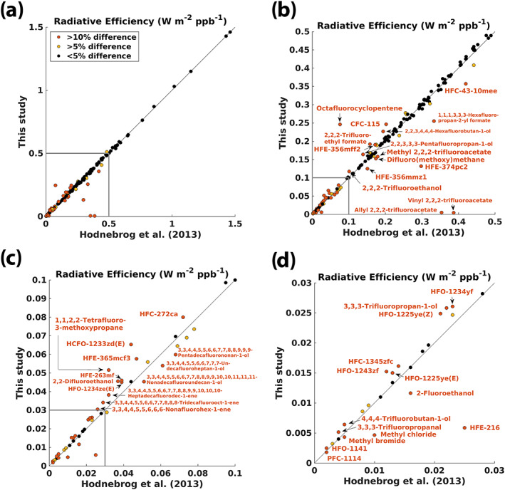
Comparison of radiative efficiencies (W m⁻² ppb⁻¹) calculated in this study (lifetime‐corrected adjusted cloudy‐sky) and from H2013 for (a) all compounds and (b)–(d) zoomed in using different scales for the RE. Black dots represent compounds where the RE in this study is less than 5% different from H2013, while yellow and red dots represent compounds where the REs are significantly different (>5% and >10%, respectively). Red dots have been labeled and represent compounds where the RE calculated here is more than 10% different from H2013.

We have adopted recommended atmospheric lifetimes from the literature and, when available, calculated GWP values. In the main part of the paper (Tables 3 and 5) we have chosen to show only GWPs for a 100‐year time horizon in addition to the lifetimes and RE values. However, many metrics exist, and the choice of metric and time horizon depends on the context in which they are used (see section 2.5). Table 16 of H2013 presented GWP values for 20, 100, and 500 year time horizons in addition to GTPs for 20, 50, and 100 year time horizons for a selection of compounds. Table 6 shows updated numbers for these compounds, and (A)GWP and (A)GTP values for the same time horizons are given for all compounds in the supporting information.

Table 6.

GWP and GTP for Selected Gases

				GWP			GTP
Identifier/name	Formula	Lifetime (yr)	RE (W m−2 ppb−1)	20‐yr	100‐yr	500‐yr	20‐yr	50‐yr	100‐yr
CFC‐11	CCl3F	52.0	0.26	7,720	5,870	2,060	7,930	6,020	3,410
CFC‐12	CCl2F2	102.0	0.32	11,800	11,800	5,610	12,900	12,600	1,000
CFC‐113	CCl2FCClF2	93.0	0.30	7,130	6,900	3,120	7,700	7,330	5,620
HCFC‐22	CHClF2	11.9	0.21	5,900	2,060	616	4,000	814	419
HCFC‐141b	CH3CCl2F	9.4	0.16	2,800	903	270	1,640	275	180
HCFC‐142b	CH3CClF2	18.0	0.19	5,720	2,410	725	4,680	1,510	564
HFC‐23	CHF3	228.0	0.19	12,900	15,500	11,600	14,400	16,400	16,300
HFC‐134a	CH2FCF3	14.0	0.17	4,300	1,600	480	3,160	767	337
HFC‐152a	CH3CHF2	1.6	0.10	607	172	52	76	37	33
1,1,1‐Trichloroethane	CH3CCl3	5.0	0.06	585	169	51	190	37	33
Tetrachloromethane	CCl4	32.0	0.17	3,960	2,310	724	3,770	2,110	880
Sulfur hexafluoride	SF6	3,200.0	0.57	19,100	26,700	37,600	21,900	27,700	32,900
PFC‐14	CF4	50,000.0	0.10	5,520	7,830	11,700	6,350	8,120	9,740

In principle, and as noted by H2013, it would be desirable to calculate the Effective Radiative Forcing (ERF) (Myhre et al., 2013) which includes rapid adjustments beyond stratospheric temperature; ERF better represents the ultimate impact of a gas on surface temperature. It remains impracticable to calculate ERF for the gases discussed here (see Shine and Myhre, 2020 for discussion) because ERF requires computationally expensive calculations using general circulation models. The radiation codes in these models do not have sufficient spectral resolution to properly represent differences between the many halocarbons presented here, and the model's unforced variability would be much larger than the RF at their current, or likely future, concentrations. Although excellent progress has been made in understanding the generic nature of rapid adjustments and intermodel differences for many climate forcing agents (e.g., Smith et al., 2018), this has not yet extended to the halocarbons in a way that would allow a reliable generic correction to be made to the RFs calculated here.

One interesting potential consequence of revisions in the GWP(100) of halocarbons is the impact on existing legislation. For example, the European Union's legislation on the usage of fluorinated greenhouse gases (EUR‐Lex, 2014), in part, puts restrictions on usages of gases based on their GWP(100); it places dates on prohibition of marketing certain equipment which uses products with GWP(100) values exceeding 150, 1,500, and 2,500. Within that legislation, the GWP(100) values are clearly defined as those mostly originating from AR4 (Forster et al., 2007), but it does not appear to account for the uncertainties inherent in those GWP(100) values. Some of the updates presented here would push gases that were on one side of these GWP(100) boundaries to the other side. For example, HFC‐152a has now breached the 150 boundary (172 compared to 138), and HFC‐134a has breached the 1,500 boundary (1,600 compared to 1,300). Hence, future updates to legislation would either have to stick to using outdated values, amend the boundaries between allowed and prohibited fluorinated gases, or else decide that some gases that were previously accepted for certain usages, are no longer so. Similarly, Japan's “Act on Rational Use and Proper Management of Fluorocarbons” has target values for GWP(100) (at values of 100, 150, 750, and 1,500) for different products (MEGJ, 2016) as does Canada's “Ozone‐depleting Substances and Halocarbon Alternatives Regulations” (MJGC, 2019), with various products limited at different values of GWP(100) (150, 750, 1,400, 1,500, and 2,200). Table 7 gives an overview of the six (out of the 40 most abundant) compounds that enter a new policy category due to our updated GWP(100) values. All six compounds show higher GWP(100) than in H2013, and updates to lifetimes and the AGWP_CO2(100) explain most of the increase for these compounds. A considerable part of the GWP(100) increase due to updated AGWP_CO2(100) (around 5% out of the 14%) arises solely because of increasing CO₂ concentrations and thereby reduced radiative efficiency of CO₂ since H2013 (see section 2.5). Hence, it can be anticipated that continued accumulation of CO₂ in the atmosphere will lead to changes in GWP values for weak atmospheric absorbers also in future updates.

Table 7.

List of compounds (among the 40 most abundant presented in Table 3) that enter new policy categories due to updated GWP(100) values

Identifier/name	Formula	H2013 GWP(100)	New GWP(100)	Policy category change	Reasons for GWP(100) change (%)
					AGWPCO2	τ	IRF curve	STA	Spectra
HCFC‐142b	CH3CClF2	1,980	2,410	Exceeds the 2,200 threshold in Canada.	+14	+5	−1	+3	+1
HFC‐32	CH2F2	677	809	Exceeds the 750 threshold in Japan and Canada	+14	+4	−1	0	+2
HFC‐134a	CH2FCF3	1,300	1,600	Exceeds the 1,500 threshold in EU, Japan and Canada	+14	+5	0	+2	+2
HFC‐152a	CH3CHF2	138	172	Exceeds the 150 threshold in EU, Japan and Canada	+14	+8	−1	+2	+1
Carbon tetrachloride	CCl4	1,730	2,310	Exceeds the 2,200 threshold in Canada	+14	+21	−2	−1	0
Halon‐2402	CBrF2CBrF2	1,470	2,280	Exceeds the 1,500 threshold in EU and Japan, and the 2,200 threshold in Canada	+14	+38	−1	−1	+1

Note. See section 4 for a discussion of, and references to, the policies that are referred to here, and section 3.1 for discussion of changes in lifetime and RE estimates. The rightmost column shows the contribution of change in GWP(100) due to the different factors: new AGWP_CO2, new lifetime estimate (τ), new instantaneous RF “Pinnock curve” (IRF curve), new method to account for stratospheric temperature adjustment (STA), and addition of absorption spectra.

Finally, we have combined our new updated RE values with present‐day atmospheric concentrations of halocarbons to determine their radiative forcing. We find that the most abundant halocarbons cause a present‐day RF of 0.38 [0.33 to 0.43] W m⁻², compared to 0.36 [0.32 to 0.40] W m⁻² in AR5 (Myhre et al., 2013) and this is almost 20% of the preindustrial (1750) to present‐day (2019) RF due to CO₂. Most of the increase in halocarbon forcing since AR5 can be attributed to increasing concentrations of CFC replacement compounds (HCFCs and HFCs) which more than outweigh the forcing due to decreasing concentrations of CFCs. However, the stronger halocarbon RF is also a consequence of updated RE values, which are slightly higher compared to AR5 for some of the most abundant compounds.

Supporting information

Supporting Information S1

Table S1

Hodnebrog, Ø. , Aamaas, B. , Fuglestvedt, J. S. , Marston, G. , Myhre, G. , & Nielsen, C. J. , et al. (2020). Updated global warming potentials and radiative efficiencies of halocarbons and other weak atmospheric absorbers. Reviews of Geophysics, 58, e2019RG000691 10.1029/2019RG000691

References

- Allen, M. R. , Fuglestvedt, J. S. , Shine, K. P. , Reisinger, A. , Pierrehumbert, R. T. , & Forster, P. M. (2016). New use of global warming potentials to compare cumulative and short‐lived climate pollutants. Nature Climate Change, 6(8), 773–776. 10.1038/nclimate2998 [DOI] [Google Scholar]
- Allen, M. R. , Shine, K. P. , Fuglestvedt, J. S. , Millar, R. J. , Cain, M. , Frame, D. J. , & Macey, A. H. (2018). A solution to the misrepresentations of CO2‐equivalent emissions of short‐lived climate pollutants under ambitious mitigation. Climate and Atmospheric Sciences, 1(1), 16 10.1038/s41612-018-0026-8 [DOI] [Google Scholar]
- Andersen, M. P. S. , Blake, D. R. , Rowland, F. S. , Hurley, M. D. , & Wallington, T. J. (2009). Atmospheric chemistry of sulfuryl fluoride: reaction with OH radicals, CI atoms and O3, atmospheric lifetime, IR spectrum, and global warming potential. Environmental Science & Technology, 43(4), 1067–1070. 10.1021/es802439f [DOI] [PubMed] [Google Scholar]
- Andersen, M. P. S. , Kyte, M. , Andersen, S. T. , Nielsen, C. J. , & Nielsen, O. J. (2017). Atmospheric chemistry of (CF3)2CFCN: A replacement compound for the most potent industrial greenhouse gas, SF6 . Environmental Science & Technology, 51(3), 1321–1329. 10.1021/acs.est.6b03758 [DOI] [PubMed] [Google Scholar]
- Ballard, J. , Knight, R. J. , Newnham, D. A. , Vander Auwera, J. , Herman, M. , Di Lonardo, G. , Masciarelli, G. , Nicolaisen, F. M. , Beukes, J. A. , Christensen, L. K. , McPheat, R. , Duxbury, G. , Freckleton, R. , & Shine, K. P. (2000a). An intercomparison of laboratory measurements of absorption cross‐sections and integrated absorption intensities for HCFC‐22. Journal of Quantitative Spectroscopy and Radiation Transfer, 66(2), 109–128. 10.1016/s0022-4073(99)00211-3 [DOI] [Google Scholar]
- Ballard, J. , Knight, R. J. , Newnham, D. A. , Vander Auwera, J. , Herman, M. , DiLonardo, G. , Masciarelli, G. , Nicolaisen, F. M. , Buekes, J. A. , Christiansen, L. K. , Duxbury, G. , McPheat, R. , Shine, K. P. , Highwood, E. J. , Freckleton, R. , Bruning, C. , & Swagg (2000b). SWAGG project—Introduction. Journal of Quantitative Spectroscopy and Radiation Transfer, 66(2), 107–108. [Google Scholar]
- Bera, P. P. , Francisco, J. S. , & Lee, T. J. (2009). Identifying the molecular origin of global warming. The Journal of Physical Chemistry A, 113(45), 12,694–12,699. 10.1021/jp905097g [DOI] [PubMed] [Google Scholar]
- Bernard, F. , Papanastasiou, D. K. , Papadimitriou, V. C. , & Burkholder, J. B. (2018). Infrared absorption spectra of N (CxF2x+1)3 x = 2−5 perfluoroamines. Journal of Quantitative Spectroscopy and Radiation Transfer, 211, 166–171. 10.1016/j.jqsrt.2018.02.039 [DOI] [Google Scholar]
- Betowski, D. , Bevington, C. , & Allison, T. C. (2016). Estimation of radiative efficiency of chemicals with potentially significant global warming potential. Environmental Science & Technology, 50(2), 790–797. 10.1021/acs.est.5b04154 [DOI] [PubMed] [Google Scholar]
- Blazquez, S. , Antinolo, M. , Nielsen, O. J. , Albaladejo, J. , & Jimenez, E. (2017). Reaction kinetics of (CF3)2CFCN with OH radicals as a function of temperature (278–358 K): A good replacement for greenhouse SF6? Chemical Physics Letters, 687, 297–302. 10.1016/j.cplett.2017.09.039 [DOI] [Google Scholar]
- Boucher, O. (2012). Comparison of physically‐and economically‐based CO2‐equivalences for methane. Earth System Dynamics, 3(1), 49–61. 10.5194/esd-3-49-2012 [DOI] [Google Scholar]
- Boucher, O. , & Reddy, M. S. (2008). Climate trade‐off between black carbon and carbon dioxide emissions. Energy Policy, 193–200. 10.1016/j.enpol.2007.08.039 [DOI] [Google Scholar]
- Bravo, I. , Aranda, A. , Hurley, M. D. , Marston, G. , Nutt, D. R. , Shine, K. P. , Smith, K. , & Wallington, T. J. (2010). Infrared absorption spectra, radiative efficiencies, and global warming potentials of perfluorocarbons: Comparison between experiment and theory. Journal of Geophysical Research, 115, D24317 10.1029/2010JD014771 [DOI] [Google Scholar]
- Butler, J. H. , & Montzka, S. A. (2020). The NOAA annual greenhouse gas index (AGGI), https://www.esrl.noaa.gov/gmd/aggi/aggi.html, last access: June 11, 2020.
- Cain, M. , Lynch, J. , Allen, M. R. , Fuglestvedt, J. S. , Frame, D. J. , & Macey, A. H. (2019). Improved calculation of warming‐equivalent emissions for short‐lived climate pollutants. Climate and Atmospheric Sciences, 2, 29 10.1038/s41612-019-0086-4 [DOI] [PMC free article] [PubMed] [Google Scholar]
- Christidis, N. , Hurley, M. D. , Pinnock, S. , Shine, K. P. , & Wallington, T. J. (1997). Radiative forcing of climate change by CFC‐11 and possible CFC‐replacements. Journal of Geophysical Research, 102(D16), 19,597–19,609. 10.1029/97JD01137 [DOI] [Google Scholar]
- Collins, W. D. , Feldman, D. R. , Kuo, C. , & Nguyen, N. H. (2018). Large regional shortwave forcing by anthropogenic methane informed by Jovian observations. Science Advances, 4, eaas9593 10.1126/sciadv.aas9593 [DOI] [PMC free article] [PubMed] [Google Scholar]
- Collins, W. D. , Ramaswamy, V. , Schwarzkopf, M. D. , Sun, Y. , Portmann, R. W. , Fu, Q. , Casanova, S. E. B. , Dufresne, J. L. , Fillmore, D. W. , Forster, P. M. D. , Galin, V. Y. , Gohar, L. K. , Ingram, W. J. , Kratz, D. P. , Lefebvre, M. P. , Li, J. , Marquet, P. , Oinas, V. , Tsushima, Y. , Uchiyama, T. , & Zhong, W. Y. (2006). Radiative forcing by well‐mixed greenhouse gases: Estimates from climate models in the Intergovernmental Panel on Climate Change (IPCC) Fourth Assessment Report (AR4). Journal of Geophysical Research, 111, D14317 10.1029/2005JD006713 [DOI] [Google Scholar]
- Collins, W. J. , Derwent, R. G. , Johnson, C. E. , & Stevenson, D. S. (2002). The oxidation of organic compounds in the troposphere and their global warming potentials. Climatic Change, 52(4), 453–479. 10.1023/a:1014221225434 [DOI] [Google Scholar]
- Collins, W. J. , Frame, D. J. , Fuglestvedt, J. , & Shine, K. P. (2019). Stable climate metrics for emissions of short and long‐lived species—Combining steps and pulses. Environmental Research Letters, 15, 024018 10.1088/1748-9326/ab6039 [DOI] [Google Scholar]
- Daniel, J. S. , Solomon, S. , & Albritton, D. L. (1995). On the evaluation of halocarbon radiative forcing and global warming potentials. Journal of Geophysical Research, 100(D1), 1271–1285. 10.1029/94JD02516 [DOI] [Google Scholar]
- Davila, K. L. , Seijas, L. E. , Almeida, R. , & Rincon, L. (2017). The performance of HF and DFT/B3LYP in the estimation of the radiative efficiencies of greenhouse gases. Journal of Computational Methods in Science and Engineering, 17(1), 187–197. 10.3233/jcm-160672 [DOI] [Google Scholar]
- Davis, M. E. , Bernard, F. , McGillen, M. R. , Fleming, E. L. , & Burkholder, J. B. (2016). UV and infrared absorption spectra, atmospheric lifetimes, and ozone depletion and global warming potentials for CCl2FCCl2F (CFC‐112), CCl3CClF2 (CFC‐112a), CCl3CF3 (CFC‐113a), and CCl2FCF3 (CFC‐114a). Atmospheric Chemistry and Physics, 16(12), 8043–8052. 10.5194/acp-16-8043-2016 [DOI] [Google Scholar]
- Etminan, M. , Highwood, E. , Laube, J. , McPheat, R. , Marston, G. , Shine, K. , & Smith, K. (2014). Infrared absorption spectra, radiative efficiencies, and global warming potentials of newly‐detected halogenated compounds: CFC‐113a, CFC‐112 and HCFC‐133a. Atmosphere, 5(3), 473–483. 10.3390/atmos5030473 [DOI] [Google Scholar]
- Etminan, M. , Myhre, G. , Highwood, E. J. , & Shine, K. P. (2016). Radiative forcing of carbon dioxide, methane, and nitrous oxide: A significant revision of the methane radiative forcing. Geophysical Research Letters, 43, 12,614–12,623. 10.1002/2016GL071930 [DOI] [Google Scholar]
- EUR‐Lex (2014). Regulation (EU) no 517/2014 of the European Parliament and of the Council of 16 April 2014 on fluorinated greenhouse gases and repealing regulation (EC) no 842/2006 text with EEA relevance, https://eur-lex.europa.eu/legal-content/en/TXT/?uri=CELEX:32014R0517
- Fisher, D. A. , Hales, C. H. , Wang, W. C. , Ko, M. K. W. , & Sze, N. D. (1990). Model‐calculations of the relative effects of CFCs and their replacements on global warming. Nature, 344(6266), 513–516. 10.1038/344513a0 [DOI] [Google Scholar]
- Forster, P. M. , Burkholder, J. B. , Clerbaux, C. , Coheur, P. F. , Dutta, M. , Gohar, L. K. , Hurley, M. D. , Myhre, G. , Portmann, R. W. , Shine, K. P. , Wallington, T. J. , & Wuebbles, D. (2005). Resolution of the uncertainties in the radiative forcing of HFC‐134a. Journal of Quantitative Spectroscopy and Radiation Transfer, 93(4), 447–460. 10.1016/j.jqsrt.2004.08.038 [DOI] [Google Scholar]
- Forster, P. M. , Ramaswamy, V. , Artaxo, P. , Berntsen, T. , Betts, R. , Fahey, D. W. , Haywood, J. , Lean, J. , Lowe, D. C. , Myhre, G. , Nganga, J. , Prinn, R. , Raga, G. , Schulz, M. , & Van Dorland, R. (2007). Changes in atmospheric constituents and in radiative forcing In Solomon S., Qin D., Manning M., Chen Z., Marquis M., et al. (Eds.), Climate change 2007: The physical science basis. Contribution of Working Group I to the Fourth Assessment Report of the Intergovernmental Panel on Climate Change, Rep. (pp. 129–234). Cambridge, United Kingdom and New York, NY, USA: Cambridge University Press. [Google Scholar]
- Freckleton, R. S. , Highwood, E. J. , Shine, K. P. , Wild, O. , Law, K. S. , & Sanderson, M. G. (1998). Greenhouse gas radiative forcing: Effects of averaging and inhomogeneities in trace gas distribution. Quarterly Journal of the Royal Meteorological Society, 124(550), 2099–2127. 10.1256/smsqj.55013 [DOI] [Google Scholar]
- Gasser, T. , Peters, G. P. , Fuglestvedt, J. S. , Collins, W. J. , Shindell, D. T. , & Ciais, P. (2017). Accounting for the climate‐carbon feedback in emission metrics. Earth System Dynamics, 8(2), 235–253. 10.5194/esd-8-235-2017 [DOI] [Google Scholar]
- Geoffroy, O. , Saint‐Martin, D. , Olivie, D. J. L. , Voldoire, A. , Bellon, G. , & Tyteca, S. (2013). Transient climate response in a two‐layer energy‐balance model. Part I: Analytical solution and parameter calibration using CMIP5 AOGCM experiments. Journal of Climate, 26(6), 1841–1857. 10.1175/jcli-d-12-00195.1 [DOI] [Google Scholar]
- Gierczak, T. , Baasandorj, M. , & Burkholder, J. B. (2014). OH + (E)‐ and (Z)‐1‐chloro‐3,3,3‐trifluoropropene‐1 (CF3CH=CHCl) reaction rate coefficients: Stereoisomer‐dependent reactivity. The Journal of Physical Chemistry A, 118(46), 11,015–11,025. 10.1021/jp509127h [DOI] [PubMed] [Google Scholar]
- Godin, P. J. , Cabaj, A. , Conway, S. , Hong, A. C. , Le Bris, K. , Mabury, S. A. , & Strong, K. (2016). Temperature‐dependent absorption cross‐sections of perfluorotributylamine. Journal of Molecular Spectroscopy, 323(Supplement C), 53–58. 10.1016/j.jms.2015.11.004 [DOI] [Google Scholar]
- Godin, P. J. , Johnson, H. , Piunno, R. , Le Bris, K. , & Strong, K. (2019). Conformational analysis and global warming potentials of 1,1,1,2,3,3‐hexafluoropropane and 1,1,2,2,3‐pentafluoropropane from absorption spectroscopy. Journal of Quantitative Spectroscopy and Radiation Transfer, 225, 337–350. 10.1016/j.jqsrt.2019.01.003 [DOI] [Google Scholar]
- Gohar, L. K. , Myhre, G. , & Shine, K. P. (2004). Updated radiative forcing estimates of four halocarbons. Journal of Geophysical Research, 109, D01107 10.1029/2003JD004320 [DOI] [Google Scholar]
- Gordon, I. E. , Rothman, L. S. , Hill, C. , Kochanov, R. V. , Tan, Y. , Bernath, P. F. , Birk, M. , Boudon, V. , Campargue, A. , Chance, K. V. , Drouin, B. J. , Flaud, J. M. , Gamache, R. R. , Hodges, J. T. , Jacquemart, D. , Perevalov, V. I. , Perrin, A. , Shine, K. P. , Smith, M. A. H. , Tennyson, J. , Toon, G. C. , Tran, H. , Tyuterev, V. G. , Barbe, A. , Csaszar, A. G. , Devi, V. M. , Furtenbacher, T. , Harrison, J. J. , Hartmann, J. M. , Jolly, A. , Johnson, T. J. , Karman, T. , Kleiner, I. , Kyuberis, A. A. , Loos, J. , Lyulin, O. M. , Massie, S. T. , Mikhailenko, S. N. , Moazzen‐Ahmadi, N. , Muller, H. S. P. , Naumenko, O. V. , Nikitin, A. V. , Polyansky, O. L. , Rey, M. , Rotger, M. , Sharpe, S. W. , Sung, K. , Starikova, E. , Tashkun, S. A. , Vander Auwera, J. , Wagner, G. , Wilzewski, J. , Wcislo, P. , Yu, S. , & Zak, E. J. (2017). The HITRAN2016 molecular spectroscopic database. Journal of Quantitative Spectroscopy and Radiation Transfer, 203, 3–69. 10.1016/j.jqsrt.2017.06.038 [DOI] [Google Scholar]
- Grossman, A. S. , Grant, K. E. , Blass, W. E. , & Wuebbles, D. J. (1997). Radiative forcing calculations for CH3Cl and CH3Br. Journal of Geophysical Research, 102(D12), 13,651–13,656. 10.1029/97JD00611 [DOI] [Google Scholar]
- Harrison, J. J. (2013). Infrared absorption cross sections for trifluoromethane. Journal of Quantitative Spectroscopy and Radiation Transfer, 130, 359–364. 10.1016/j.jqsrt.2013.05.026 [DOI] [Google Scholar]
- Harrison, J. J. (2015a). New and improved infrared absorption cross sections for dichlorodifluoromethane (CFC‐12). Atmospheric Measurement Techniques, 8(8), 3197–3207. 10.5194/amt-8-3197-2015 [DOI] [Google Scholar]
- Harrison, J. J. (2015b). Infrared absorption cross sections for 1,1,1,2‐tetrafluoroethane. Journal of Quantitative Spectroscopy and Radiation Transfer, 151, 210–216. 10.1016/j.jqsrt.2014.09.023 [DOI] [Google Scholar]
- Harrison, J. J. (2016). New and improved infrared absorption cross sections for chlorodifluoromethane (HCFC‐22). Atmospheric Measurement Techniques, 9(6), 2593–2601. 10.5194/amt-9-2593-2016 [DOI] [Google Scholar]
- Harrison, J. J. (2019). Infrared absorption cross sections for air‐broadened 1,1‐dichloro‐1‐fluoroethane (HCFC‐141b). Journal of Quantitative Spectroscopy and Radiative Transfer, 238, 106489 10.1016/j.jqsrt.2019.04.041 [DOI] [Google Scholar]
- Harrison, J. J. , Boone, C. D. , & Bernath, P. F. (2017). New and improved infra‐red absorption cross sections and ACE‐FTS retrievals of carbon tetrachloride (CCl4). Journal of Quantitative Spectroscopy and Radiative Transfer, 186(Supplement C), 139–149. 10.1016/j.jqsrt.2016.04.025 [DOI] [Google Scholar]
- Highwood, E. J. , & Shine, K. P. (2000). Radiative forcing and global warming potentials of 11 halogenated compounds. Journal of Quantitative Spectroscopy and Radiation Transfer, 66(2), 169–183. 10.1016/s0022-4073(99)00215-0 [DOI] [Google Scholar]
- Hodnebrog, Ø. , Dalsoren, S. B. , & Myhre, G. (2018). Lifetimes, direct and indirect radiative forcing, and global warming potentials of ethane (C2H6), propane (C3H8), and butane (C4H10). Atmospheric Science Letters, 19, e804 10.1002/asl.804 [DOI] [Google Scholar]
- Hodnebrog, Ø. , Etminan, M. , Fuglestvedt, J. S. , Marston, G. , Myhre, G. , Nielsen, C. J. , Shine, K. P. , & Wallington, T. J. (2013). Global warming potentials and radiative efficiencies of halocarbons and related compounds: A comprehensive review. Reviews of Geophysics, 51, 300–378. 10.1002/rog.20013 [DOI] [PMC free article] [PubMed] [Google Scholar]
- Hong, A. C. , Young, C. J. , Hurley, M. D. , Wallington, T. J. , & Mabury, S. A. (2013). Perfluorotributylamine: A novel long‐lived greenhouse gas. Geophysical Research Letters, 40, 6010–6015. 10.1002/2013GL058010 [DOI] [Google Scholar]
- Imasu, R. , Suga, A. , & Matsuno, T. (1995). Radiative effects and halocarbon global warming potentials of replacement compounds for chlorofluorocarbons. Journal of the Meteorological Society of Japan, 73(6), 1123–1136. 10.2151/jmsj1965.73.6_1123 [DOI] [Google Scholar]
- IPCC . (1990). In Houghton J. T., Jenkins G. J., & Ephraums J. J. (Eds.), Climate change: The IPCC scientific assessment (p. 410). Cambridge: Cambridge University Press. [Google Scholar]
- IPCC. (1994). In Houghton J. T., Filho L. G. M., Bruce J., Lee H., Callander B. A., Haites E. F., Harris N., & Maskell K. (Eds.), Climate change 1994: Radiative forcing of climate change and an evaluation of the IPCC IS92 emission scenarios. Cambridge, UK: Cambridge University Press. [Google Scholar]
- IPCC. (2001). In Houghton J. T., Ding Y., Griggs D. J., Noguer M., van der Linden P. J., Dai X., Maskell K., & Johnson C. A. (Eds.), Climate change 2001: The scientific basis. Contribution of Working Group I to the Third Assessment Report of the Intergovernmental Panel on Climate Change (p. 881). Cambridge, UK and New York, NY: Cambridge University Press. [Google Scholar]
- Jacquinet‐Husson, N. , Armante, R. , Scott, N. A. , Chedin, A. , Crepeau, L. , Boutammine, C. , Bouhdaoui, A. , Crevoisier, C. , Capelle, V. , Boonne, C. , Poulet‐Crovisier, N. , Barbe, A. , Benner, D. C. , Boudon, V. , Brown, L. R. , Buldyreva, J. , Campargue, A. , Coudert, L. H. , Devi, V. M. , Down, M. J. , Drouin, B. J. , Fayt, A. , Fittschen, C. , Flaud, J. M. , Gamache, R. R. , Harrison, J. J. , Hill, C. , Hodnebrog, O. , Hu, S. M. , Jacquemart, D. , Jolly, A. , Jimenez, E. , Lavrentieva, N. N. , Liu, A. W. , Lodi, L. , Lyulin, O. M. , Massie, S. T. , Mikhailenko, S. , Muller, H. S. P. , Naumenko, O. V. , Nikitin, A. , Nielsen, C. J. , Orphal, J. , Perevalov, V. I. , Perrin, A. , Polovtseva, E. , Predoi‐Cross, A. , Rotger, M. , Ruth, A. A. , Yu, S. S. , Sung, K. , Tashkun, S. A. , Tennyson, J. , Tyuterev, V. I. G. , Auwera, J. V. , Voronin, B. A. , & Makie, A. (2016). The 2015 edition of the GEISA spectroscopic database. Journal of Molecular Spectroscopy, 327, 31–72. 10.1016/j.jms.2016.06.007 [DOI] [Google Scholar]
- Jacquinet‐Husson, N. , Crepeau, L. , Armante, R. , Boutammine, C. , Chedin, A. , Scott, N. A. , Crevoisier, C. , Capelle, V. , Boone, C. , Poulet‐Crovisier, N. , Barbe, A. , Campargue, A. , Benner, D. C. , Benilan, Y. , Bezard, B. , Boudon, V. , Brown, L. R. , Coudert, L. H. , Coustenis, A. , Dana, V. , Devi, V. M. , Fally, S. , Fayt, A. , Flaud, J. M. , Goldman, A. , Herman, M. , Harris, G. J. , Jacquemart, D. , Jolly, A. , Kleiner, I. , Kleinbohl, A. , Kwabia‐Tchana, F. , Lavrentieva, N. , Lacome, N. , Xu, L. H. , Lyulin, O. M. , Mandin, J. Y. , Maki, A. , Mikhailenko, S. , Miller, C. E. , Mishina, T. , Moazzen‐Ahmadi, N. , Muller, H. S. P. , Nikitin, A. , Orphal, J. , Perevalov, V. , Perrin, A. , Petkie, D. T. , Predoi‐Cross, A. , Rinsland, C. P. , Remedios, J. J. , Rotger, M. , Smith, M. A. H. , Sung, K. , Tashkun, S. , Tennyson, J. , Toth, R. A. , Vandaele, A. C. , & Vander Auwera, J. (2011). The 2009 edition of the GEISA spectroscopic database. Journal of Quantitative Spectroscopy and Radiation Transfer, 112(15), 2395–2445. 10.1016/j.jqsrt.2011.06.004 [DOI] [Google Scholar]
- Jain, A. K. , Briegleb, B. P. , Minschwaner, K. , & Wuebbles, D. J. (2000). Radiative forcings and global warming potentials of 39 greenhouse gases. Journal of Geophysical Research, 105(D16), 20,773–20,790. 10.1029/2000JD900241 [DOI] [Google Scholar]
- Joos, F. , Roth, R. , Fuglestvedt, J. S. , Peters, G. P. , Enting, I. G. , von Bloh, W. , Brovkin, V. , Burke, E. J. , Eby, M. , Edwards, N. R. , Friedrich, T. , Frölicher, T. L. , Halloran, P. R. , Holden, P. B. , Jones, C. , Kleinen, T. , Mackenzie, F. , Matsumoto, K. , Meinshausen, M. , Plattner, G. K. , Reisinger, A. , Segschneider, J. , Shaffer, G. , Steinacher, M. , Strassmann, K. , Tanaka, K. , Timmermann, A. , & Weaver, A. J. (2013). Carbon dioxide and climate impulse response functions for the computation of greenhouse gas metrics: A multi‐model analysis. Atmospheric Chemistry and Physics, 13(5), 2793–2825. 10.5194/acp-13-2793-2013 [DOI] [Google Scholar]
- Kazakov, A. , McLinden, M. O. , & Frenkel, M. (2012). Computational design of new refrigerant fluids based on environmental, safety, and thermodynamic characteristics. Industrial & Engineering Chemistry Research, 51(38), 12,537–12,548. 10.1021/ie3016126 [DOI] [Google Scholar]
- Kochanov, R. V. , Gordon, I. E. , Rothman, L. S. , Shine, K. P. , Sharpe, S. W. , Johnson, T. J. , Wallington, T. J. , Harrison, J. J. , Bernath, P. F. , Birk, M. , Wagner, G. , Le Bris, K. , Bravo, I. , & Hill, C. (2019). Infrared absorption cross‐sections in HITRAN2016 and beyond: Expansion for climate, environment, and atmospheric applications. Journal of Quantitative Spectroscopy and Radiation Transfer, 230, 172–221. 10.1016/j.jqsrt.2019.04.001 [DOI] [Google Scholar]
- Kovács, T. , Feng, W. , Totterdill, A. , Plane, J. M. C. , Dhomse, S. , Gómez‐Martín, J. C. , Stiller, G. P. , Haenel, F. J. , Smith, C. , Forster, P. M. , García, R. R. , Marsh, D. R. , & Chipperfield, M. P. (2017). Determination of the atmospheric lifetime and global warming potential of sulfur hexafluoride using a three‐dimensional model. Atmospheric Chemistry and Physics, 17(2), 883–898. 10.5194/acp-17-883-2017 [DOI] [Google Scholar]
- Laube, J. C. , Newland, M. J. , Hogan, C. , Brenninkmeijer, C. A. M. , Fraser, P. J. , Martinerie, P. , Oram, D. E. , Reeves, C. E. , Rockmann, T. , Schwander, J. , Witrant, E. , & Sturges, W. T. (2014). Newly detected ozone‐depleting substances in the atmosphere. Nature Geoscience, 7(4), 266–269. 10.1038/ngeo2109 [DOI] [Google Scholar]
- Le Bris, K. , DeZeeuw, J. , Godin, P. J. , & Strong, K. (2018). Infrared absorption cross‐sections, radiative efficiency and global warming potential of HFC‐43‐10mee. Journal of Molecular Spectroscopy, 348, 64–67. 10.1016/j.jms.2017.06.004 [DOI] [Google Scholar]
- Le Bris, K. , & Graham, L. (2015). Quantitative comparisons of absorption cross‐section spectra and integrated intensities of HFC‐143a. Journal of Quantitative Spectroscopy and Radiative Transfer, 151(Supplement C), 13–17. 10.1016/j.jqsrt.2014.09.005 [DOI] [Google Scholar]
- Le Bris, K. , McDowell, J. , & Strong, K. (2012). Measurements of the infrared absorption cross‐sections of HCFC‐141b (CH3CFCl2). Journal of Quantitative Spectroscopy and Radiation Transfer, 113(15), 1913–1919. 10.1016/j.jqsrt.2012.05.004 [DOI] [Google Scholar]
- Le Bris, K. , & Strong, K. (2010). Temperature‐dependent absorption cross‐sections of HCFC‐142b. Journal of Quantitative Spectroscopy and Radiation Transfer, 111(3), 364–371. 10.1016/j.jqsrt.2009.10.005 [DOI] [Google Scholar]
- Massie, S. T. , Goldman, A. , McDaniel, A. H. , Cantrell, C. A. , Davidson, J. A. , Shetter, R. E. , & Calvert, J. G. (1991). Temperature dependent infrared cross sections for CFC‐11, CFC‐12, CFC‐13, CFC‐14, CFC‐22, CFC‐113, CFC‐114, and CFC‐115, 67 pp, NCAR Tech. Note NCAR/TN‐358+STR, Nat. Cent. for Atmos. Res., Boulder, Colorado.
- McDaniel, A. H. , Cantrell, C. A. , Davidson, J. A. , Shetter, R. E. , & Calvert, J. G. (1991). The temperature‐dependent, infrared‐absorption cross‐sections for the chlorofluorocarbons ‐ CFC‐11, CFC‐12, CFC‐13, CFC‐14, CFC‐22, CFC‐113, CFC‐114, and CFC‐115. Journal of Atmospheric Chemistry, 12(3), 211–227. 10.1007/BF00048074 [DOI] [Google Scholar]
- McGillen, M. R. , Bernard, F. , Fleming, E. L. , & Burkholder, J. B. (2015). HCFC‐133a (CF3CH2Cl): OH rate coefficient, UV and infrared absorption spectra, and atmospheric implications. Geophysical Research Letters, 42, 6098–6105. 10.1002/2015GL064939 [DOI] [Google Scholar]
- McLinden, M. O. , Kazakov, A. F. , Brown, J. S. , & Domanski, P. A. (2014). A thermodynamic analysis of refrigerants: Possibilities and tradeoffs for low‐GWP refrigerants. International Journal of Refrigeration‐Revue International du Froid, 38, 80–92. 10.1016/j.ijrefrig.2013.09.032 [DOI] [Google Scholar]
- MEGJ (2016). Act on rational use and proper management of fluorocarbons, ministry of the environment government of Japan, http://www.env.go.jp/en/earth/ozone/laws/ozone4.pdf
- Meinshausen, M. , Vogel, E. , Nauels, A. , Lorbacher, K. , Meinshausen, N. , Etheridge, D. M. , Fraser, P. J. , Montzka, S. A. , Rayner, P. J. , Trudinger, C. M. , Krummel, P. B. , Beyerle, U. , Canadell, J. G. , Daniel, J. S. , Enting, I. G. , Law, R. M. , Lunder, C. R. , O'Doherty, S. , Prinn, R. G. , Reimann, S. , Rubino, M. , Velders, G. J. M. , Vollmer, M. K. , Wang, R. H. J. , & Weiss, R. (2017). Historical greenhouse gas concentrations for climate modelling (CMIP6). Geoscientific Model Development, 10(5), 2057–2116. 10.5194/gmd-10-2057-2017 [DOI] [Google Scholar]
- MJGC (2019). Ozone‐depleting Substances and halocarbon alternatives regulations by Ministry of Justice Government of Canada, SOR/2016–137, https://laws-lois.justice.gc.ca/eng/regulations/SOR-2016-137/
- Molina, M. J. , & Rowland, F. S. (1974). Stratospheric sink for chlorofluoromethanes ‐ chlorine atomic‐catalysed destruction of ozone. Nature, 249(5460), 810–812. 10.1038/249810a0 [DOI] [Google Scholar]
- Myhre, G. , Highwood, E. J. , Shine, K. P. , & Stordal, F. (1998). New estimates of radiative forcing due to well mixed greenhouse gases. Geophysical Research Letters, 25(14), 2715–2718. 10.1029/98GL01908 [DOI] [Google Scholar]
- Myhre, G. , Shindell, D. , Bréon, F.‐M. , Collins, W. , Fuglestvedt, J. , Huang, J. , Koch, D. , Lamarque, J.‐F. , Lee, D. , Mendoza, B. , Nakajima, T. , Robock, A. , Stephens, G. , Takemura, T. , & Zhang, H. (2013). Anthropogenic and natural radiative forcing In Stocker T. F., Qin D., Plattner G.‐K., Tignor M., Allen S. K., Boschung J., Nauels A., Xia Y., Bex V., & Midgley P. M. (Eds.), Climate change 2013: The physical science basis Contribution of Working Group I to the Fifth Assessment Report of the Intergovernmental Panel on Climate Change (pp. 659–740). Cambridge, UK and New York, NY: Cambridge University Press; 10.1017/CBO9781107415324.018 [DOI] [Google Scholar]
- Myhre, G. , & Stordal, F. (1997). Role of spatial and temporal variations in the computation of radiative forcing and GWP. Journal of Geophysical Research, 102(D10), 11,181–11,200. 10.1029/97JD00148 [DOI] [Google Scholar]
- Nemtchinov, V. , & Varanasi, P. (2003). Thermal infrared absorption cross‐sections of CCl4 needed for atmospheric remote sensing. Journal of Quantitative Spectroscopy and Radiation Transfer, 82(1–4), 473–481. 10.1016/s0022-4073(03)00171-7 [DOI] [Google Scholar]
- Olivié D. J. L., & Peters, G. P. (2013). Variation in emission metrics due to variation in CO2 and temperature impulse response functions. Earth System Dynamics, 4(2), 267–286. 10.5194/esd-4-267-2013 [DOI] [Google Scholar]
- Oreopoulos, L. , Mlawer, E. , Delamere, J. , Shippert, T. , Cole, J. , Fomin, B. , Iacono, M. , Jin, Z. H. , Li, J. N. , Manners, J. , Raisanen, P. , Rose, F. , Zhang, Y. C. , Wilson, M. J. , & Rossow, W. B. (2012). The continual intercomparison of radiation codes: Results from phase I. Journal of Geophysical Research, 117, D06117 10.1029/2011JD016821 [DOI] [Google Scholar]
- Orkin, V. L. , Khamaganov, V. G. , & Guschin, A. G. (2014). Photochemical properties of hydrofluoroethers CH3OCHF2, CH3OCF3, and CHF2OCH2CF3: Reactivity toward OH, IR absorption cross sections, atmospheric lifetimes, and global warming potentials. The Journal of Physical Chemistry A, 118(45), 10,770–10,777. 10.1021/jp506377w [DOI] [PubMed] [Google Scholar]
- Papadimitriou, V. C. , McGillen, M. R. , Smith, S. C. , Jubb, A. M. , Portmann, R. W. , Hall, B. D. , Fleming, E. L. , Jackman, C. H. , & Burkholder, J. B. (2013). 1,2‐Dichlorohexafluoro‐cyclobutane (1,2‐c‐C4F6Cl2, R‐316c) a potent ozone depleting substance and greenhouse gas: Atmospheric loss processes, lifetimes, and ozone depletion and global warming potentials for the (E) and (Z) stereoisomers. The Journal of Physical Chemistry A, 117(43), 11,049–11,065. 10.1021/jp407823k [DOI] [PubMed] [Google Scholar]
- Papanastasiou, D. K. , Beltrone, A. , Marshall, P. , & Burkholder, J. B. (2018). Global warming potential estimates for the C1–C3 hydrochlorofluorocarbons (HCFCs) included in the Kigali amendment to the Montreal protocol. Atmospheric Chemistry and Physics, 18(9), 6317–6330. 10.5194/acp-18-6317-2018 [DOI] [Google Scholar]
- Pinnock, S. , Hurley, M. D. , Shine, K. P. , Wallington, T. J. , & Smyth, T. J. (1995). Radiative forcing of climate by hydrochlorofluorocarbons and hydrofluorocarbons. Journal of Geophysical Research, 100(D11), 23,227–23,238. 10.1029/95JD02323 [DOI] [Google Scholar]
- Ravishankara, A. R. , Solomon, S. , Turnipseed, A. A. , & Warren, R. F. (1993). Atmospheric lifetimes of long‐lived halogenated species. Science, 259(5092), 194–199. 10.1126/science.259.5092.194 [DOI] [PubMed] [Google Scholar]
- Ray, E. A. , Moore, F. L. , Elkins, J. W. , Rosenlof, K. H. , Laube, J. C. , Rockmann, T. , Marsh, D. R. , & Andrews, A. E. (2017). Quantification of the SF6 lifetime based on mesospheric loss measured in the stratospheric polar vortex. Journal of Geophysical Research: Atmospheres, 122, 4626–4638. 10.1002/2016JD026198 [DOI] [Google Scholar]
- Reisinger, A. , Meinshausen, M. , Manning, M. , & Bodeker, G. (2010). Uncertainties of global warming metrics: CO2 and CH4 . Geophysical Research Letters, 37, L14707 10.1029/2010GL043803 [DOI] [Google Scholar]
- Robson, J. I. , Gohar, L. K. , Hurley, M. D. , Shine, K. P. , & Wallington, T. J. (2006). Revised IR spectrum, radiative efficiency and global warming potential of nitrogen trifluoride. Geophysical Research Letters, 33, L10817 10.1029/2006GL026210 [DOI] [Google Scholar]
- Rogelj, J. , & Schleussner, C.‐F. (2019). Unintentional unfairness when applying new greenhouse gas emissions metrics at country level. Environmental Research Letters, 14, 114039 10.1088/1748-9326/ab4928 [DOI] [Google Scholar]
- Rothman, L. S. , Gordon, I. E. , Barbe, A. , Benner, D. C. , Bernath, P. E. , Birk, M. , Boudon, V. , Brown, L. R. , Campargue, A. , Champion, J. P. , Chance, K. , Coudert, L. H. , Dana, V. , Devi, V. M. , Fally, S. , Flaud, J. M. , Gamache, R. R. , Goldman, A. , Jacquemart, D. , Kleiner, I. , Lacome, N. , Lafferty, W. J. , Mandin, J. Y. , Massie, S. T. , Mikhailenko, S. N. , Miller, C. E. , Moazzen‐Ahmadi, N. , Naumenko, O. V. , Nikitin, A. V. , Orphal, J. , Perevalov, V. I. , Perrin, A. , Predoi‐Cross, A. , Rinsland, C. P. , Rotger, M. , Simeckova, M. , Smith, M. A. H. , Sung, K. , Tashkun, S. A. , Tennyson, J. , Toth, R. A. , Vandaele, A. C. , & Vander Auwera, J. (2009). The HITRAN 2008 molecular spectroscopic database. Journal of Quantitative Spectroscopy and Radiation Transfer, 110(9–10), 533–572. 10.1016/j.jqsrt.2009.02.013 [DOI] [Google Scholar]
- Schlabach, M. , van Bavel, B. , Lomba, J. A. B. , Borgen, A. , Gabrielsen, G. W. , Götsch, A. , Halse, A. K. , Hanssen, L. , Krogseth, I. S. , Nikiforov, V. , Nygård, T. , Nizzetto, P. B. , Reid, M. J. , Rostkowski, P. , & Samanipour, S. (2018). Screening programme 2017‐AMAP assessment compounds, Report funded by The Norwegian Environment Agency, ISBN: 978-82-425-2940-4
- Sharpe, S. W. , Johnson, T. J. , Sams, R. L. , Chu, P. M. , Rhoderick, G. C. , & Johnson, P. A. (2004). Gas‐phase databases for quantitative infrared spectroscopy. Applied Spectroscopy, 58(12), 1452–1461. 10.1366/0003702042641281 [DOI] [PubMed] [Google Scholar]
- Shine, K. P. , Fuglestvedt, J. S. , Hailemariam, K. , & Stuber, N. (2005). Alternatives to the global warming potential for comparing climate impacts of emissions of greenhouse gases. Climatic Change, 68(3), 281–302. 10.1007/s10584-005-1146-9 [DOI] [Google Scholar]
- Shine, K. P. , & Myhre, G. (2020). The spectral nature of stratospheric temperature adjustment and its application to halocarbon radiative forcing. Journal of Advances in Modeling Earth Systems, 12, e2019MS001951 10.1029/2019MS001951 [DOI] [Google Scholar]
- Sihra, K. , Hurley, M. D. , Shine, K. P. , & Wallington, T. J. (2001). Updated radiative forcing estimates of 65 halocarbons and nonmethane hydrocarbons. Journal of Geophysical Research, 106(D17), 20,493–20,505. 10.1029/2000JD900716 [DOI] [Google Scholar]
- Smith, C.,. J. , Kramer, R. J. , Myhre, G. , Forster, P. M. , Soden, B. J. , Andrews, T. , Boucher, O. , Faluvegi, G. , Flaschner, D. , Hodnebrog, O. , Kasoar, M. , Kharin, V. , Kirkevag, A. , Lamarque, J. F. , Mulmenstadt, J. , Olivie, D. , Richardson, T. , Samset, B. H. , Shindell, D. , Stier, P. , Takemura, T. , Voulgarakis, A. , & Watson‐Parris, D. (2018). Understanding rapid adjustments to diverse forcing agents. Geophysical Research Letters, 45, 12,023–12,031. 10.1029/2018GL079826 [DOI] [PMC free article] [PubMed] [Google Scholar]
- SPARC (2013). Report on the lifetimes of stratospheric ozone‐depleting substances, their replacements, and related species, Ko M., Newman P., Reimann S., Strahan S. (Eds.), SPARC Report No. 6, WCRP‐15/2013, SPARC Office; https://www.sparc-climate.org/publications/sparc-reports/sparc-report-no-6/ [Google Scholar]
- Taylor, K. E. , Stouffer, R. J. , & Meehl, G. A. (2011). An overview of CMIP5 and the experiment design. Bulletin of the American Meteorological Society, 93(4), 485–498. 10.1175/BAMS-D-11-00094.1 [DOI] [Google Scholar]
- Totterdill, A. , Kovacs, T. , Feng, W. H. , Dhomse, S. , Smith, C. J. , Gomez‐Martin, J. C. , Chipperfield, M. P. , Forster, P. M. , & Plane, J. M. C. (2016). Atmospheric lifetimes, infrared absorption spectra, radiative forcings and global warming potentials of NF3 and CF3CF2Cl (CFC‐115). Atmospheric Chemistry and Physics, 16(17), 11,451–11,463. 10.5194/acp-16-11451-2016 [DOI] [Google Scholar]
- UNFCCC (2019). Report of the conference of the parties serving as the meeting of the parties to the Paris agreement on the third part of its first session, held in Katowice from 2 to 15 December 2018. PA/CMA/2018/3/Add.2 , https://unfccc.int/sites/default/files/resource/cma2018_3_add2_new_advance.pdf
- Vander Auwera, J. (2000). Infrared absorption cross‐sections for two substituted ethanes: 1,1‐difluoroethane (HFC‐152a) and 1,2‐dichloroethane. Journal of Quantitative Spectroscopy and Radiation Transfer, 66(2), 143–151. 10.1016/S0022-4073(99)00213-7 [DOI] [Google Scholar]
- Velders, G. J. M. , & Daniel, J. S. (2014). Uncertainty analysis of projections of ozone‐depleting substances: Mixing ratios, EESC, ODPs, and GWPs. Atmospheric Chemistry and Physics, 14(6), 2757–2776. 10.5194/acp-14-2757-2014 [DOI] [Google Scholar]
- Wallington, T. J. , Pivesso, B. P. , Lira, A. M. , Anderson, J. E. , Nielsen, C. J. , Andersen, N. H. , & Hodnebrog, Ø. (2016). CH3Cl, CH2Cl2, CHCl3, and CCl4: Infrared spectra, radiative efficiencies, and global warming potentials. Journal of Quantitative Spectroscopy and Radiative Transfer, 174(Supplement C), 56–64. 10.1016/j.jqsrt.2016.01.029 [DOI] [Google Scholar]
- WMO (2011). Scientific assessment of ozone depletion: 2010, global ozone research and monitoring project—Report no. 50, 572 pp., World Meteorological Organization, Geneva, Switzerland.
- WMO (2015). Scientific assessment of ozone depletion: 2014, global ozone research and monitoring project—Report no. 55, 416 pp., World Meteorological Organization, Geneva, Switzerland.
- WMO (2019). Scientific assessment of ozone depletion: 2018, global ozone research and monitoring project—Report no. 58, 588 pp., World Meteorological Organization, Geneva, Switzerland.
- WMO/GAW (2019). WMO greenhouse gas bulletin. Number 15, 25 November 2019. https://library.wmo.int/doc_num.php?explnum_id=10100
- Wuebbles, D. J. , Jain, A. K. , Patten, K. O. , & Grant, K. E. (1995). Sensitivity of direct global warming potentials to key uncertainties. Climatic Change, 29(3), 265–297. 10.1007/bf01091865 [DOI] [Google Scholar]
- Zhang, H. , Wu, J. X. , & Shen, Z. P. (2011). Radiative forcing and global warming potential of perfluorocarbons and sulfur hexafluoride. Science China Earth Sciences, 54(5), 764–772. 10.1007/s11430-010-4155-0 [DOI] [Google Scholar]
- Zhang, N. , Uchimaru, T. , Guo, Q. , Qing, F. , Chen, L. , & Mizukado, J. (2017). Atmospheric chemistry of perfluorocyclopentene (cyc‐CF2CF2CF2CF=CF−): Kinetics, products and mechanism of gas‐phase reactions with OH radicals, and atmospheric implications. Atmospheric Environment, 160(Supplement C), 46–54. 10.1016/j.atmosenv.2017.04.012 [DOI] [Google Scholar]
Associated Data
This section collects any data citations, data availability statements, or supplementary materials included in this article.
Supplementary Materials