Computational Tools for Evaluating Phylogenetic and Hierarchical Clustering Trees

Abstract

Inferential summaries of tree estimates are useful in the setting of evolutionary biology, where phylogenetic trees have been built from DNA data since the 1960s. In bioinformatics, psychometrics, and data mining, hierarchical clustering techniques output the same mathematical objects, and practitioners have similar questions about the stability and “generalizability” of these summaries. This article describes the implementation of the geometric distance between trees developed by Billera, Holmes, and Vogtmann (2001) equally applicable to phylogenetic trees and hierarchical clustering trees, and shows some of the applications in evaluating tree estimates.

In particular, since Billera et al. (2001) have shown that the space of trees is negatively curved (called a CAT(0) space), a collection of trees can naturally be represented as a tree. We compare this representation to the Euclidean approximations of treespace made available through both a classical multidimensional scaling and a Kernel multidimensional scaling of the matrix of the distances between trees. We also provide applications of the distances between trees to hierarchical clustering trees constructed from microarrays. Our method gives a new way of evaluating the influence of both certain columns (positions, variables, or genes) and certain rows (species, observations, or arrays) on the construction of such trees. It also can provide a way of detecting heterogeneous mixtures in the input data. Supplementary materials for this article are available online.

1. INTRODUCTION

Binary rooted trees are used as parameters in evolutionary studies while hierarchical clustering trees are the most popular display for microarray data. From a mathematical point of view, these objects are the same: semi-labeled rooted binary trees. However, few multivariate methods are available for building confidence regions around estimated trees of this type. Here, we propose two methods for evaluating variability in such tree estimates.

Throughout this article, we use a natural distance between trees that was introduced and studied by Billera, Holmes, and Vogtmann (2001). Recent advances in the encoding of the problem (Staple 2003) and its solution in polynomial time (Owen and Provan 2010) now allow us to compute the BHV distances between hundreds of trees. The present article describes the first available implementation of these advances and some applications.

We will focus on rooted, weighted binary trees, resulting from either phylogenetic inferences based on DNA, or hierarchical clustering trees, commonly resulting from microarray data. These trees present a common structure: they have known entities at the leaves, for instance contemporary species of bacteria or known genes. These leaves come with data associated to them, either nucleotide sequences for a given set of species or gene expression patterns across a set of patients. We will suppose that the data corresponding to each leaf are combined to form the rows of a matrix X.

Each edge of the rooted tree defines a clade—the group of leaves below that edge. We also use the term split to describe the bipartition induced by removing that edge. Rooted binary trees with labels at the leaves can have different branching patterns. For instance, consider a tree with three leaves labeled 1, 2, and 3. There are three different branching patterns: one groups 2 and 3 in a clade with 1 as the outgroup, another groups 1 and 3 in a clade with 2 as the outgroup, and the last groups 1 and 2 in a clade with 3 as the outgroup. Current practices in evaluating tree estimates lean on a simple unidimensional summary: the proportion of times a clade occurs in a bootstrap resampling scheme or a sample from a Bayesian posterior distribution. These proportions are recorded either as the binomial rates along the edges of the tree (Felsenstein 1983) or as a set of bin frequencies of the competing trees’ branching patterns considered as categorical output.

In this article, we propose several alternative evaluation procedures, all geometric, based on distances between trees. The idea of comparing trees through a notion of distance between trees has many variations. Robinson and Foulds (1981) proposed a coarse distance between phylogenetic trees that provides only integer values. This was used, for instance, in post-processing trees by Stockham, Wang, and Warnow (2002). Waterman and Smith (1978) proposed the Nearest Neighbor Interchange (NNI) as a biologically reasonable distance between trees. We will use the distance of Billera, Holmes, and Vogtmann (2001) and call it the BHV distance, denoted d_BHV. This distance can be considered a continuous refinement of NNI when one takes into account the edge lengths of the trees. The BHV distance also represents the geodesic path length in the geometric tree space developed by Billera, Holmes, and Vogtmann (2001); this intuitively corresponds to the minimum length of a continuous deformation of one tree to another. We do not explain this distance carefully here (see the original article by Billera, Holmes, and Vogtmann 2001, or the expositiory accounts by Holmes 2003a or Holmes 2003b).

Heat map bi-clustering representations, made popular in microarray analyses, can also benefit from multivariate evaluations. To motivate our development, we present a small example.

Example 1: Hierarchical Clustering variability.

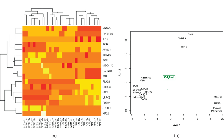
Hierarchical clustering trees such as those in Figure 1(a) are called biclustering heatmaps (Wilkinson and Friendly 2009). The figure shows both a clustering of patients (the columns in this data) and the genes (the rows). We will consider the analysis done by removing each gene in turn and recomputing the patient cluster trees. We then use these as points in a multivariate plot.

Figure 1.

Cross-validation of the rows allows us to geometrically study the effect of individual genes.(a) Hierarchical clustering trees of rows (genes) and columns (patients) of a microarray matrix. (b) Plot of cross-validated hierarchical clustering trees. Each point represents a tree that was estimated without the gene it is labeled with.

We will use cross-validation to see how the clustering trees change when each of the genes is removed: we generate 16 new datasets by deleting each row (representing a gene) in turn and using these new data to generate distances from which a new tree is estimated. This gives us 16 “cross-validated” trees and the original tree. The axes are the first and second coordinates output from an embedding of the tree-points in a Euclidean space constructed using the method developed in Section 3. The groupings of the tree-points show that some genes have similar effects on the estimates when missing. Figure 1(b) shows the cross-validated trees with the original tree at the center of the triangular scatter of points. The point labels are the names of the genes that were deleted from the dataset for that particular tree estimate. Notice that the cross-validated tree-points can be seen to form three clusters, indicating that genes in each cluster cause similar effects to the tree when removed. We will return to this example in Section 3.5 in the context of computing what we call the gene’s “leverage.”

The rest of the article is organized as follows. In the next section, we survey current practices in evaluating tree parameters in a statistical context. We do this for both evolutionary studies and hierarchical clustering approaches in multivariate analyses. The first part of the Appendix in the Supplementary Material (online) contains a more detailed review of tree estimation in the phylogenetic setting.

A brief description of the distance implementation is provided in Section 2.4 and a detailed account of the algorithm, precise encoding choices, and optimization schemes are given online in the second section of the Supplementary Material. Section 3 shows how to use multidimensional scaling to approximately embed the trees in a Euclidean space. We give examples using multidimensional representations for comparing trees generated from different data, and for comparing cross-validated data for detecting influential variables in hierarchical clustering. Section 4 shows how to embed the trees in a tree, providing a robust method for detecting mixtures.

Section 5 shows how paths between trees can be used to find the boundary points between two different branching patterns. These paths are built using a simulated annealing algorithm and can also provide the boundary data used by Efron, Halloran, and Holmes (1996) to correct the bias in the naïve bootstrap for trees (Holmes 2003a).

2. BASIC USES OF TREE PARAMETERS

In this section, we will place the question of evaluating trees in the context of statistical estimation and give an overview of current practices of evaluation. The data from which the tree is estimated are a n × p matrix, with n being the number of observations for the hierarchical clustering studies or the number of species for the phylogenetic examples, and p being the number of genes or the number of characters.

2.1. Methods For Estimating Trees

2.1.1. Statistical Inference for Phylogenetic Trees.

Phylogenetic trees are estimates of a statistical tree parameter (the family tree of the species present) under certain assumptions on the evolutionary process that changes the nucleotides over time. The data used to estimate the trees are the row-vectors of characters, usually representing DNA nucleotides {a, c, g, t} or a binary variable {0, 1}. We provide a review of references and current methodology in the Supplementary Material (online).

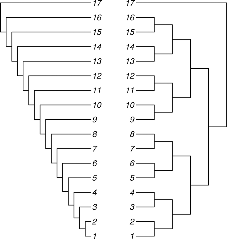
Figure 2 shows two extreme tree shapes; we call the one on the left the comb tree and the one on the right the balanced tree.

Figure 2.

The tree on the left is the comb tree on 17 leaves, and the tree on the right is called the balanced tree on 17 leaves.

2.2. Hierarchical Clustering Trees

Hierarchical clustering trees are built from distances or dissimilarities between the rows of the data matrix (Hartigan 1967). Common examples include computations of dissimilarities in gene expression or in occurrence of words in texts or web pages. The resulting hierarchical clustering tree has the advantage over simple partitioning methods that one can look at the output to make an informed decision as to the relevant number of clusters for a particular dataset.

Microarray studies have popularized the use of a double hierarchical clustering or biclustering trees where both the rows and columns of the data are clustered in the margins of a heatmap representation of either the similarities or the raw data. Although this is the most popular method for visualizing both relations between genes and patient groups in gene expression studies (Carr, Somogyi, and Michaels 1997; Eisen et al. 1998), it was developed earlier by several statisticians (for an interesting review of this “post-genomic icon,” see Wilkinson and Friendly 2009). Many implementations are available; the illustration in Figure 1 was made with heatmap function in R (Ihaka and Gentleman 1996; see online Supplementary Material for the code and data).

2.3. Methods For Generating Trees

With advances in computational power we can use simulated data to evaluate clustering stability, either in a frequentist (Bootstrap) setting or by using a Bayesian paradigm, where trees from a posterior distribution can be generated by Markov Chain Monte Carlo (MCMC) methods or tree estimation methods.

We provide here a brief overview of the standard methods for generating distributions of trees. Different approaches to the problem of combining the trees are summarized. This combination of information on different trees is a nonstandard statistical problem because trees do not lie in a Euclidean space (Billera, Holmes, and Vogtmann 2001).

Bootstrap support for phylogenies.

The application of the bootstrap technique (Efron 1979) to the phylogenetic tree problem is done by taking columns of the matrix of aligned sequences as the objects to bootstrap (with columns representing character positions and rows representing species). The sampling distribution of the estimated tree is estimated by resampling with replacement among the characters or columns of the data. This provides a large set of plausible alternative datasets, each used in the same way as the original data to give a new tree (see Holmes 2003a for a review). These trees were used by Felsenstein (1983) to build a confidence statement relevant to each inner edge of the tree. Each inner edge defines a split of the leaves into two sets. Felsenstein proposed using the estimate of the binomial frequencies of the split across all bootstraps as a measure of confidence of an edge; an improvement was proposed by Efron, Halloran, and Holmes (1996). This adjustment uses a path between trees that are on each side of the boundary separating two tree topologies; we show in Section 3.2 how this can be implemented using our geometric distance.

Parametric bootstrapping for microarray clusters.

Kerr and Churchill (2001) proposed a way of validating hierarchical clustering as it is used in microarray analysis. Their model is a parametric ANOVA model for microarrays that includes gene, dye, and array effects. Once these effects have been estimated on the data, simulated data incorporating realistic noise distributions can be generated through a parametric bootstrap type procedure. From the simulated data, many hierarchical clusters are generated and then compared. The authors use this to evaluate the stability of a gene, using the percent of bootstrap clusterings in which it matches to the same cluster in the same way Felsenstein (1983) provided the estimate of the binomial proportion of trees with a given clade. We can repeat their generation process but combine the trees differently. We show in Section 3 how a more multivariate approach can provide richer visualizations of the stability of hierarchical clustering trees.

Bayesian posterior distributions for phylogenetic trees.

Yang and Rannala (1997) developed the Bayesian framework for estimating phylogenetic trees. The posterior distribution provides an estimate of variability. The usual models put prior distributions on the DNA mutation rates that occur during the evolutionary process and a uniform distribution on the original tree and proceed through the use of MCMC to generate instances of the posterior distribution. Implementations such as MrBayes (Huelsenbeck and Ronquist 2001) provide a sample of trees from the posterior distribution. These can be used for the same purpose as the bootstrap resample of trees. Following the procedures explained in Section 3, we combine these picks from the posterior distribution using the distances to give an estimate of a median posterior tree as well as a multivariate representation.

Bayesian methods in hierarchical clustering.

Savage et al. (2009) provided a Bayesian nonparametric method for generating posterior distributions of hierarchical clustering trees. Visualizing such posterior distributions can be tackled with the same tools as those used for Bayesian phylogenetics.

2.4. Computing The BHV Distance

The max-flow optimization algorithm proposed by Owen and Provan (2010) allows us to compute the geodesic distance metric proposed by Billera, Holmes, and Vogtmann (2001). This distance metric arises naturally from the formulation of tree space as a space made up of Euclidean orthants. A path between two trees consists of line segments through a sequence of orthants. This sequence of orthants is the path space. A path is a geodesic when it has the smallest length of all paths between two points.

Billera, Holmes, and Vogtmann (2001) showed that tree space is negatively curved; as a consequence, there is a unique geodesic between any two trees (Gromov 1987). We can find the distance between two trees by finding the geodesic path between them. The advances used in our program recast this problem as the maximization of paths in a bipartite graph (Staple 2003; Owen and Provan 2010). Section B of the Supplementary Material (online) contains a detailed description of the implementation. A specific coding of the tree edge compatibilities as a graph is explained in detail. The algorithm has been implemented in the R package distory (Chakerian and Holmes 2010), which also contains many of the examples from this article. The package requires the ape (Paradis 2006) package for analyzing phylogenetic trees and can be beneficially supplemented by the phangorn (Schliep 2009) package.

The current implementation in distory can compute all pairwise distances between 200 bootstrap replicates of a 146-leaf tree in approximately 2 min on a Core 2 Duo 1.6 GHz processor, giving a rate of over 300 distance calculations per second.

3. CHOOSING A GEOMETRY FOR EMBEDDING TREES

This section gives three examples of the use of the BHV distance. As background, Billera, Holmes, and Vogtmann (2001) showed that the distance as computed in distory endows the space of trees with a negative curvature. This means that the tree points are not naturally embeddable in a Euclidean space (see the excellent book length treatment of nonpositively curved metric spaces by Bridson and Haefliger 1999). An illustration of the reason for this is attempted in Figure 3.

Figure 3.

Three triangles illustrating nonpositively curved spaces. The center illustration represents three points (trees) in treespace, a, b, and c, with the geodesics running between them. Notice the paths are made of sequences of linear segments that sit in the Euclidean cubes of the cube complex, but together the geodesic path has an overall negative curvature (the triangles are thin compared to the Euclidean comparison triangle on the right). The left triangle depicts the extreme situation in which the space is so negatively curved as to be a tree.

A question raised by Figure 3 is whether we can make a good approximate representation of many trees given their BHV distances by embedding the points in a Euclidean space using a modified multidimensional scaling approach or whether it is better to place the trees in a tree, as we do in Section 4 of this article. The question of choice between spatial and treelike representations is an old one and was clearly posed by Pruzansky, Tversky, and Carroll (1982) almost 30 years ago in the context of dissimilarities measured on psychological preferences. These points are illustrated below.

3.1. Multidimensional Scaling And Its Application To Tree Comparisons

Psychometricians, ecologists, and statisticians have long favored a method known as classical multidimensional scaling (MDS) to approximate general dissimilarities with Euclidean distances. We refer the reader to the standard exposition by Mardia, Kent, and Bibby (1979) who explained how to find the best k-dimensional Euclidean space such that the points in this space have distances approximating a given distance matrix as well as possible.

Distances between trees are not globally Euclidean. However, two trees that only differ in their branch lengths, not in their branching patters, are contained in the same Euclidean cube of dimension n − 2, where n is the number of leaves of the tree. Distances between two trees that have very similar branching patterns are close to being Euclidean. This motivates using a kernel modification of MDS where we use a kernel built from the distance between two trees τ_x and τ_y as k(τ_x, τ_y) = exp(−d(τ_x, τ_y)). The multidimensional scaling analysis of this kernelized similarity will provide a representation where points that are close together have their distances well approximated whereas points far apart just appear far without jeopardizing the overall optimization (see Williams 2000, for a comparison between kernel Principal Component Analysis (PCA) and classical MDS).

3.2. MDS Of Bootstrapped Trees

As we have seen in Section 2, one approach to inference for hierarchical clustering and phylogenetic trees is to simply apply a nonparametric resampling bootstrap to the data and re-estimate the trees. This gives an idea of the overall variability of the data under the assumption that the unknown distribution of the distances $d(\tau ,\widehat{\tau })$ can be well approximated by that of $d\left(\widehat{\tau },{\widehat{\tau }}^{*}\right)$, where ${\widehat{\tau }}^{*}$ denotes the bootstrapped estimates of the tree.

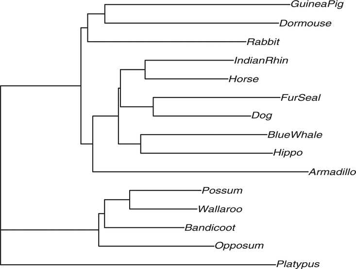
Here, we will make a MDS plot of the bootstrap tree estimates. We provide as an example a study using the Laurasiatheria data (Lin et al. 2002) that can be accessed from the package phangorn (Schliep 2009). The data consist of a group of placental mammals believed to have originated on the northern supercontinent of Laurasia. Our study dataset includes a subset of these mammals, with the platypus considered an outgroup used to root the tree. The tree as estimated on the original data is represented in Figure 4. For demonstration purposes, we have used the minimum evolution algorithm (Desper and Gascuel 2002) to estimate the tree.

Figure 4.

A tree estimated from aligned sequences of length 3179.

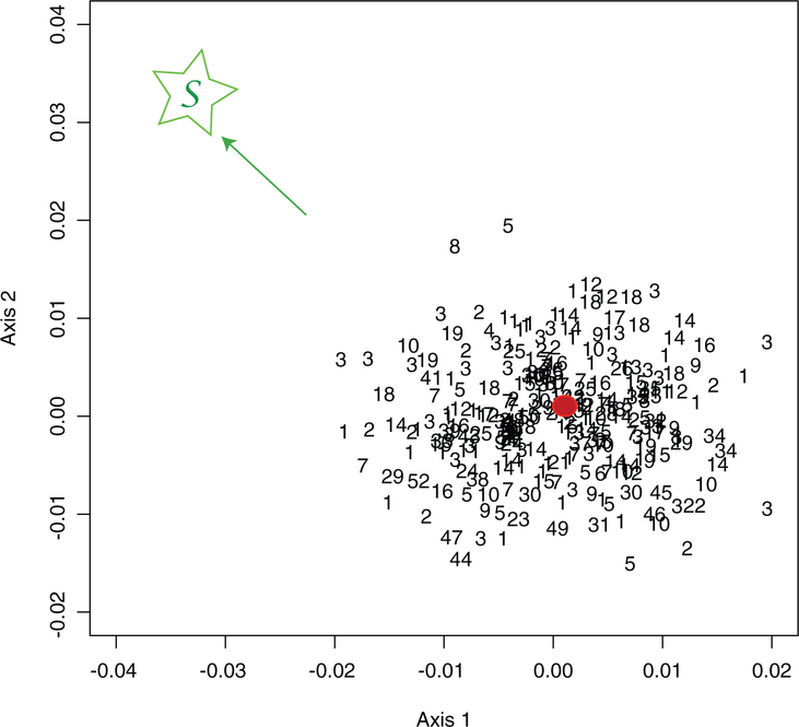
In one of these runs generating 250 bootstrap trees, there were about 50 different branching patterns. An MDS plot of the first two principal coordinates using the BHV distance is presented in Figure 5. The code to reproduce this analysis is available in the Supplementary Material (online).

Figure 5.

First MDS plane representing 250 bootstraps. The tree topologies were numbered from 1 to 52. The red bullet is the original tree, the green S is in the direction of the star tree.

The estimate from the original data, projected as a red bullet, is at the center of the scatterplot in Figure 5, leading us to believe that this estimate is unbiased. We have also chosen to represent a star tree on the plot. This star tree was constructed by making its inner edges zero and giving the pendant edges lengths equal to the distances of the leaves to the root. This tree is projected as the point labeled by S (in green), at the extreme left of the plot.

Notice that the additional star tree is projected far from the bootstrap scatter thus enabling us to conclude that the true tree is not close to being an unresolved star tree.

When comparing two random variables, we build a confidence interval for the difference, and if 0 is in the confidence interval we conclude that the variables are not significantly different. In Figure 5, the projection of the star tree S is outside the outer convex hull of the projected points; we can conclude from this that the probability that the star tree belongs to the bootstrap confidence region is very low. If the star tree was central to the confidence region, then we could conclude that the data are not treelike and that the tree is unresolved in the sense of not having well-distinguished interior edges.

This is a concrete implementation of the idea of using convex hulls to make confidence statements of this type (Holmes 2005).

As an aside, note that the numbers in Figure 5 label the different types of branching patterns. We see that trees of the same topology are not necessarily closer to each other using the BHV distance without further adjustments. In some cases, we may want to add an extra penalty for crossing orthants (i.e., changing branching patterns or tree topologies). We give examples of such modifications of the distance in the Chakerian and Holmes (2010) vignette.

3.3. Variability Of Trees From a Bayesian Posterior Distribution

After running MCMC Bayesian sampling from the posterior such as that available in MrBayes (Huelsenbeck and Ronquist 2001), we obtain several sets of trees from different runs of the chain.¹ To evaluate these runs, we took 250 random picks from the two runs combined, with the first 200,000 trees from each run discarded. Each MCMC was run 1,000,000 times on the same subset of the Laurasiatherian data available in the phangorn package (Schliep 2009).

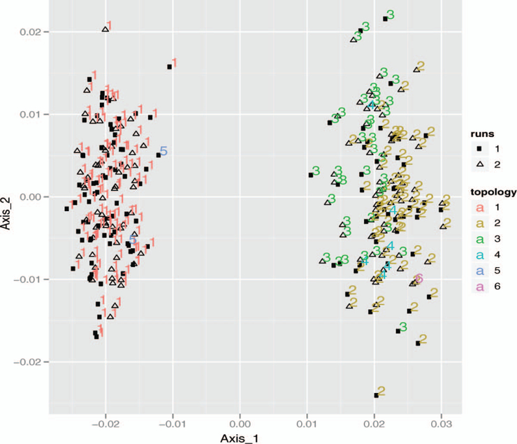
The standard MDS plot is shown in Figure 6. We see that the scatterplot is bimodal, but that this cannot be explained by the runs; in fact, the figure does a nice job of showing how well the MCMC runs have mixed, since the two runs are indistinguishable

Figure 6.

First plane of MDS plot (41%) of the trees sampled from the Bayesian posterior. The color indicates branching pattern and the glyph indicates the run number.

There were six different branching patterns in all. We have colored each of these with one of six colors. Figure 6 shows an equal distribution of branching patterns between runs.

3.4. Studying a Mutation Rate Gradient On Bethe Trees

Here, we show an example of using these multivariate MDS representations in a parametric bootstrap setting. Erdős et al. (1999) have shown that the tree shape that requires the longest sequence length for inferring the root sequence accurately is the balanced tree. Mossel (2004) recognized this tree shape as the Bethe lattice, known in statistical mechanics, and used available theory to give bounds on the sequence lengths necessary to rebuild the tree accurately with a given probability. For this shape, Mossel (2004) showed that if mutation rates are high it is impossible to reconstruct ancestral data at the root and the topology of large phylogenetic trees from a number of characters smaller than a low-degree polynomial in the number of leaves.

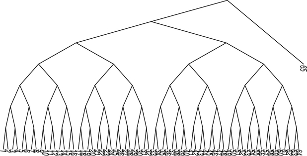
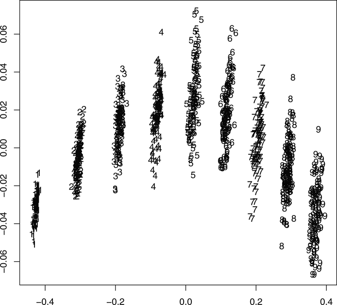
We generated 100 sets of sequence data for each of nine different mutation rates from α = 0.01 to α = 0.09, all from the same Bethe lattice tree as represented in Figure 7. For each of the 900 datasets, we estimated one phylogenetic tree using maximum likelihood. The true tree was added as a 901st tree and distances between all the trees was computed. Figure 8 shows the first two principal coordinates of all 901 trees as they were obtained through a classical MDS. The original tree is the empty circle point in the left hand clusters of 1s. We see a typical arch shape, which is a classical instance of the horseshoe phenomenon (Diaconis, Goel, and Holmes 2007) in the presence of an underlying gradient. In this case, the gradient is the mutation rate. It is an open question as to whether such a plot could be useful in the inverse problem of trying to estimate the relevant mutation rate for a dataset, given the bootstrapped trees generated using the parametric bootstrap with differing mutation rates.

Figure 7.

A balanced tree on 64 leaves, known as the Bethe lattice. We have added an outgroup to fix the root.

Figure 8.

The first two axes of the MDS of 901 trees with mutation rates varying from α = 0.01 to α = 0.09 (labeled as 100 × α). The online version of this figure is in color.

3.5. Finding Inconsistent Characters With High Leverage

In regression it is often useful to find outlying observations, often defined as those observations that have high leverage. Leverage may be quantified using Cook’s distance that measures the effect of deleting a given observation (Cook 1977). In the context of regression, the formula is:

$$D_i=\frac{{{\sum }_{j=1}^n\left({\widehat{Y}}_j-{\widehat{Y}}_j^{\left(i\right)}\right)}^2}{p\text{MSE}}.$$

Where Ŷ is the response estimated with the full sample and Ŷ⁽ⁱ⁾ is the estimate that is computed without observation (i). Data points with large values of D_i have high leverage and may distort the outcome and accuracy of a regression. Points with a large Cook’s distance are often considered outliers needing further study. High leverage in regression can be detected by seeing a large jump in the fitted model after the point is taken out.

In our context, we would take a value D_i proportional to the average squared distances between the estimated tree and the tree without the point whose leverage we are computing:

$$D_i\propto \sum _{j=1}^n{d}^2\left({\widehat{\tau }}_j,{\widehat{\tau }}_j^{(i)}\right).$$

In the phylogenetic context, if a character or a set of contiguous characters are taken out of the data and the tree changes significantly, this can be an indication of recombination or horizontal transfer events. In previous work, de Oliveira Martins, Leal, and Kishino (2008) used the the minimum number of subtree prune-and-regraft (SPR) operations required to resolve inconsistencies between two trees to detect recombination events along DNA sequences in HIV. Our approach is simpler since we will not use a Bayesian posterior, just the distance between the original tree and the tree without that particular character/segment.

In the hierarchical clustering context, Figure 1 in the first example shows the MDS plot built from distances between each of the cross-validation datasets built by excluding a single gene and recomputing the hierarchical clustering tree and then computing the BHV distance between trees. Each cross-validated tree is labeled by the gene that is excluded. Table 2 in the Supplementary Material (online) shows the distances between the cross-validated trees and the original tree. If we consider the distances to the original tree in the first row as shown in Table 1, we can see that they are basically bimodal, a group around distance 17 from the original tree and a group of values around 20. The plot in Figure 1 tells a richer story since it shows how the genes can be organized into three clusters according to the effect they have on the overall hierarchical clustering tree. In some sense, this gives us a more geometric picture of the leverage of each gene.

Table 1.

Rounded distances between the cross-validated trees and the original tree

	SNN	AF.	PLAG	DHR	PASK	PDE	CAC	LRR	F2R	CX3.	MAD.	PPP.	KIF	MGC	BCR	IFI.	TRIM
Ori.	22	17	23	20	17	21	16	16	16	16	22	22	16	18	17	21	17

4. TREE OF TREES

A tree itself is a negatively curved space (Gromov 1987). The space of all trees is also a negatively curved space represented by the intermediary situation in Figure 3. Instead of taking the Euclidean approach shown in the right-most triangle, we can consider taking the alternative, the left triangle, which is itself a tree. We thus suggest that a tree of trees would be a useful representation of a sample from the Bayesian posterior or a bootstrap resampling distribution of trees. Such a representation was generated by Stockham, Wang, and Warnow (2002) using a different discrete distance as a method for post-processing trees.

4.1. Mixture Detection

A particularly interesting application of the use of the tree of trees is the detection of mixtures of the evolutionary processes from a set of aligned sequences. Evolutionary mixtures pose problems when using MCMC methods in the Bayesian estimation context (Mossel and Vigoda 2005). These authors noted that MCMC methods such as those used to compute Bayesian posterior distributions on trees can be misleading when the data are generated from a mixture of trees, because in the case of a “well-balanced” mixture the algorithms are not guaranteed to converge, or may take an exponential number of steps to do so. They recommended separating the sequences according to coherent evolutionary processes. However, this adds a step to the process; ideally we would like to be able to use the original data to detect the mixture. Suppose the data come from the mixture of several different trees; we will see how the bootstrap and the various distances and representations can detect these in the simple case of a mixture of two evolutionary processes.

Suppose we have K trees τ₁, τ₂, …, τ_K generated from one original alignment either by bootstrapping the original data or by using an MCMC method for generating them from the Bayesian posterior. We use the distance between trees to make a hierarchical clustering tree using single linkage (the distance between two clusters is computed as the distance between the two closest elements in the two clusters (Hartigan 1975)). This provides a picture of the relationships between the trees.

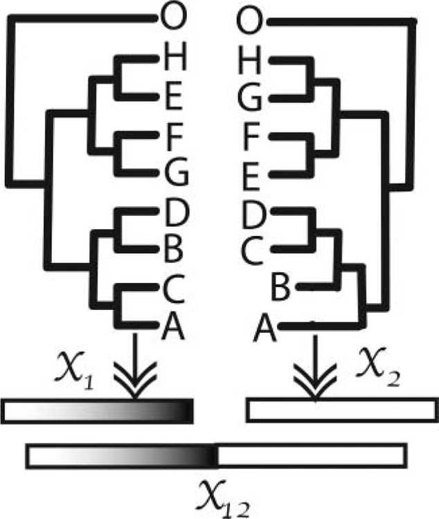
In this simulated example, we generate two sets of data of length 1000 from the two different trees as plotted in Figure 9.

Figure 9.

Trees used to generate sequences of length 1000 each that are combined into one 2000 long aligned set ${\mathcal{X}}_{12}$.

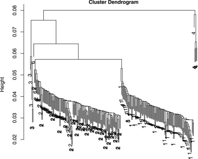
We concatenate this generated sequence data into one dataset ${\mathcal{X}}_{12}$ on which the standard phylogenetic estimation procedures are run. This provides the estimated phylogenetic tree for the data. We then generate 250 bootstrap resamples from the combined data, and compute the BHV distances between the 250 trees from each of the bootstrap resamples, using these to make a hierarchical clustering single linkage tree from this distance matrix. We see in Figure 10 that the tree shows two very distinct classes of about the same size and a few stray classes marked 3, 4, and 6, whereas the tree branching order labeled 5 is incorporated into the group of 1’s (numbers represent tree topologies). We can infer from this clustering pattern that the data came from two main evolutionary components ${\mathcal{X}}_1$ and ${\mathcal{X}}_2$ that correspond to the two trees in Figure 9. Tracking which positions were resampled more frequently in each of the clusters could then allow us to recover which positions “belonged” to each original tree.

Figure 10.

Hierarchical clustering of 250 trees resulting from a nonparametric bootstrap of the data generated by the double dataset ${\mathcal{X}}_{12}$. The numbers represent the phylogenetic branching pattern types, of which there were six in this simulation.

5. USING THE PATH BETWEEN TWO TREES TO FIND BOUNDARIES

It can be useful to explore both the neighborhood of a given tree and the datasets that are borderline in the sense that small perturbations induce a change in the tree topology. Comparison of two borderline datasets will indicate which columns/characters cause the trees to flip from one branching pattern to another. This provides complementary information on the characters that are instrumental in causing one topology to occur rather than another, thus enabling a more complete interpretation of the variability in tree sampling distributions.

5.1. Borderline Trees

How close the tree estimate is to being borderline, in a particular sense of closeness to a different tree, provides meaningful information on the estimate’s stability. Evaluating the distance between a tree and the boundary between two different branching pattern orthants is done by creating small perturbations of the original data by bootstrapping. If all the bootstrap resamples give the same tree, then we are sure that the estimate we have is not “borderline,” that is, the topology of the estimate is the same as that of the true tree.

However, if the bootstrap resamples give many different trees showing an even distribution in a very large region, this indicates that the original data are not very treelike and the inferred tree has many competing neighbors.

In fact, if the star tree with all edges equal to zero is close to the original tree then the number of alternatives will be exponentially large (Holmes 2005). If r contiguous edges of the tree are small, there will still be (2r − 3)!! = (2r − 3) × (2r – 5) × · · · × 3 × 1 trees in its close neighborhood.

In the case of the bootstrap analysis of the Laurasiatherian dataset, we found that there are actually nine trees in the bootstrap resample that are borderline neighbors to the original tree. These neighbors and their respective BHV distances to the original tree are presented in the Supplementary Material (online; Figure 12). We see that there are thus many “small edges” in this particular tree estimate, and the original estimated tree shares boundaries with nine competing orthants, indicating that the estimation process is very unstable.

5.2. Finding Borderline Data With MCMC

We can use MCMC methods to help with the following question: Given a target tree (e.g., a tree that lies on the border between two orthants of interest), how can we find a configuration of weights for the columns of the original sequences such that the tree estimated from this re-weighted data is as close as possible to the target tree?

We start with the original aligned sequences organized as a matrix with p columns, c₁, c₂, …, c_p, the original weights are k⁰ = (1, 1, 1, …, 1).

We then draw proposals by increasing the count of one position by one and decreasing the count of another by one; that is, make elementary steps of the form

$$\mathbf{\text{k}}=\left(k_1,k_2,k_3,\dots ,k_p\right)\to {\mathbf{\text{k}}}^{\prime }=\left(k_1,k_2,k_3,\dots k_j-1,\dots k_i+1,\dots ,k_p\right).$$

With i and j chosen uniformly from between 1 and p. This maintains the number of columns in the dataset. A tree is estimated with the proposed changed weights k′, and the BHV distance to the target tree is computed. The proposal is accepted or rejected based on the ratio of the old distance to the new distance (if the new distance is smaller, the ratio is greater than 1, so the proposal is accepted automatically; if the new distance is greater, with some probability the proposal is accepted anyway to allow the MCMC to get out of local minima). A simulated annealing scheme (Kirkpatrick 1984) introduces a temperature that is used to gradually decrease the acceptance probability, and helps with the location of a closest approximating set of positions. These positions are then reported along with the resulting tree and the final distance. This algorithm has been implemented in R (Ihaka and Gentleman 1996) and is available in the distory (Chakerian and Holmes 2010) package. The method is useful in implementing an improved version of correcting for the bias in the bootstrap procedure for trees [see Efron, Halloran, and Holmes (1996) for the justification of this correction term].

6. SUMMARY AND OPEN RESEARCH QUESTIONS

We have combined the problems of evaluating phylogenetic trees and hierarchical clustering displays in a common mathematical framework. Since tree space geometry sits somewhere in between tree geometry and Euclidean geometry, the two methods we have developed provide complementary views of collections of trees.

We have shown simple applications in evaluating distributions of trees as output by Bayesian posterior sampling or bootstrap methods. By embedding rooted binary trees in a metric space associated to a Euclidean approximation provided by MDS we can capitalize on all the existing methods in multivariate statistics, from linear discriminant analysis to k-means clustering, to make useful nonparametric summaries. On the other hand, by embedding the trees themselves in a tree we can detect mixtures and hierarchical structures in the sampling distributions.

We have thus shown through examples that a computable, detailed distance between trees can provide valuable information about the variability of tree estimates and a substitute notion of multivariate spread, as well as providing a nonparametric way of testing whether an evolutionary process is treelike. A major question that merits further research concerns realistic probability measures on treespace, and how such a measure should be used to provide useful priors and a theoretical notion of variance (and more general moments) for the space.

In multivariate analysis it is often important to account for differing levels of variability in the data by rescaling variables, as one does in linear discriminant analysis for instance. In the context of phylogenetic trees, in the case where the contemporary DNA sequences are used to build trees that go far back in the past, it seems natural to ask if it would not be better to put different weights on the branches of the tree to compensate for the higher uncertainty with which we infer what is happening high up (toward the root) of the tree (Mossel 2004). In the same way, we rescale variables so they have the same variance before doing a multivariate analysis. We would divide the edges in the tree closer to the root with larger numbers corresponding to the larger uncertainty, so that large differences higher in the tree would be downweighted since we are not sure of them. Examples of this differential weighting can be found in the vignette that accompanies the package distory (Chakerian and Holmes 2010), but no statistical theory has yet been developed to guide the choice of such weights.

REFERENCES

- Billera L, Holmes S, and Vogtmann K (2001), “The Geometry of Tree Space,” Advances in Applied Mathematics, 27, 771–801. [Google Scholar]
- Bridson MR, and Haefliger A (1999), Metric Spaces of Non-Positive Curvature, Berlin: Springer-Verlag. [Google Scholar]
- Carr DB, Somogyi R, and Michaels G (1997), “Templates for Looking at Gene Expression Clustering,” Statistical Computing & Statistical Graphics Newsletter, 7, 20–29. [Google Scholar]
- Chakerian J, and Holmes S (2010), Distory: Distances Between Trees. Available at: http://cran.r-project.org/web/packages/distory/index.html.
- Cook RD (1977), “Detection of Influential Observation in Linear Regression,” Technometrics, 19 (1), 15–18. [Google Scholar]
- de Oliveira Martins L, Leal E, and Kishino H (2008), “Phylogenetic Detection of Recombination With a Bayesian Prior on the Distance Between Trees,” PLoS ONE, 3 (7), e2651. [DOI] [PMC free article] [PubMed] [Google Scholar]
- Desper R, and Gascuel O (2002), “Fast and Accurate Phylogeny Reconstruction Algorithms Based on the Minimum-Evolution Principle,” Journal of Computational Biology, 9 (5), 687–705. [DOI] [PubMed] [Google Scholar]
- Diaconis P, Goel S, and Holmes S (2007), “Horseshoes in Multidimensional Scaling and Kernel Methods,” Annals of Applied Statistics, 2, 777–807. [Google Scholar]
- Efron B (1979), “Bootstrap Methods: Another Look at the Jackknife,” The Annals of Statistics, 7, 1–26. [Google Scholar]
- Efron B, Halloran E, and Holmes SP (1996), “Bootstrap Confidence Levels for Phylogenetic Trees,” Proceedings of the National Academy of Sciences of the United States of America, 93, 13429–13434. [DOI] [PMC free article] [PubMed] [Google Scholar]
- Eisen MB, Spellman PT, Brown PO, and Botstein D (1998), “Cluster Analysis and Display of Genome-Wide Expression Patterns,” Proceedings of the National Academy of Sciences of the United States of America, 95 (25), 14863. [DOI] [PMC free article] [PubMed] [Google Scholar]
- Erdős PL, Steel MA, Székely LA, and Warnow TJ (1999), “A Few Logs Suffice to Build (Almost) All Trees: I,” Random Structures Algorithms, 14 (2), 153–184. [Google Scholar]
- Felsenstein J (1983), “Statistical Inference of Phylogenies” (with discussion), Journal of the Royal Statistical Society, Series A, 146, 246–272. [Google Scholar]
- Gromov M (1987), “Hyperbolic Groups,” in Essays in Group Theory, New York: Springer, pp. 75–263. [Google Scholar]
- Hartigan J (1967), “Representation of Similarity Matrices by Trees,” Journal of the American Statistical Association, 62, 1140–1158. [Google Scholar]
- Hartigan JA (1975), Clustering Algorithms, New York: Wiley. [Google Scholar]
- Holmes S (2003a), “Bootstrapping Phylogenetic Trees: Theory and Methods,” Statistical Science, 18 (2), 241–255. [Google Scholar]
- Holmes S (2003b), “Statistics for Phylogenetic Trees,” Theoretical Population Biology, 63 (1), 17–32. [DOI] [PubMed] [Google Scholar]
- Holmes S (2005), “Statistical Approach to Tests Involving Phylogenies,” in Mathematics of Evolution and Phylogeny, Oxford: Oxford University Press, pp. 91–120. [Google Scholar]
- Huelsenbeck J, and Ronquist F (2001), “MrBayes: Bayesian Inference of Phylogenetic Trees,” Bioinformatics,17, 754–755. [DOI] [PubMed] [Google Scholar]
- Ihaka R, and Gentleman R (1996), “R: A Language for Data Analysis and Graphics,” Journal of Computational and Graphical Statistics, 5 (3), 299–314. [Google Scholar]
- Kerr MK, and Churchill GA (2001), “Bootstrapping Cluster Analysis: Assessing the Reliability of Conclusions From Microarray Experiments,” Proceedings of the National Academy of Sciences of the United States of America, 98 (16), 8961–8965. [DOI] [PMC free article] [PubMed] [Google Scholar]
- Kirkpatrick S (1984), “Optimization by Simulated Annealing: Quantitative Studies,” Journal of Statistical Physics, 34, 975–986. [Google Scholar]
- Lin YH, McLenachan PA, Gore AR, Phillips MJ, Ota R, Hendy MD, and Penny D (2002), “Four New Mitochondrial Genomes and the Increased Stability of Evolutionary Trees of Mammals From Improved Taxon Sampling,” Molecular Biology and Evolution, 19 (12), 2060–2070. [DOI] [PubMed] [Google Scholar]
- Mardia K, Kent J, and Bibby J (1979), Multivariate Analysis, New York: Academic Press. [Google Scholar]
- Mossel E (2004), “Phase Transitions in Phylogeny,” Transactions of American Mathematical Society, 356 (6),2379–2404. [Google Scholar]
- Mossel E, and Vigoda E (2005), “Phylogenetic MCMC Algorithms are Misleading on Mixtures of Trees,” Science, 309 (5744), 2207–2209. [DOI] [PubMed] [Google Scholar]
- Owen M, and Provan JS (2010), “A Fast Algorithm for Computing Geodesic Distances in Tree Space,” IEEE/ACM Transactions on Computational Biology and Bioinformatics, 8, 2–13. [DOI] [PubMed] [Google Scholar]
- Paradis E (2006), Analysis of Phylogenetics and Evolution With R, New York: Springer. [Google Scholar]
- Pruzansky S, Tversky A, and Carroll J (1982), “Spatial Versus Tree Representations of Proximity Data,” Psychometrika, 47, 3–24. [Google Scholar]
- Robinson DF, and Foulds LR (1981), “Comparison of Phylogenetic Trees,” Mathematical Biosciences, 53(1–2), 131–147. [Google Scholar]
- Savage R, Heller K, Xu Y, and Ghahramani Z (2009), “R/BHC: Fast Bayesian Hierarchical Clustering for Microarray Data,” BMC, Bioinformatics, 10, 242. [DOI] [PMC free article] [PubMed] [Google Scholar]
- Schliep K (2009), Phangorn: Phylogenetic Analysis in R. Available at: http://cran.r-project.org/web/packages/phangorn/index.html. [DOI] [PMC free article] [PubMed]
- Staple A (2003), “Computational Advances in Distance Between Trees,” unpublished undergraduate thesis, Statistics Department, Stanford University. [Google Scholar]
- Stockham C, Wang LS, and Warnow T (2002), “Statistically Based Postprocessing of Phylogenetic Analysis by Clustering,” Bioinformatics, 18, S285–S293. [DOI] [PubMed] [Google Scholar]
- Waterman MS, and Smith TF (1978), “On the Similarity of Dendrograms,” Journal of Theoretical Biology,73 (4), 789–800. [DOI] [PubMed] [Google Scholar]
- Wilkinson L, and Friendly M (2009), “The History of the Cluster Heat Map,” The American Statistician, 63 (2),179–184. [Google Scholar]
- Williams CK (2000), “On a Connection Between Kernel PCA and Metric Multidimensional Scaling,” NIPS,13, 675–681. [Google Scholar]
- Yang Z, and Rannala B (1997), “Bayesian Phylogenetic Inference Using DNA Sequences: A Markov Chain Monte Carlo Method,” Molecular Biology and Evolution, 14, 717–724. [DOI] [PubMed] [Google Scholar]
Associated Data
This section collects any data citations, data availability statements, or supplementary materials included in this article.