2-CHANNEL CONVOLUTIONAL 3D DEEP NEURAL NETWORK (2CC3D) FOR FMRI ANALYSIS: ASD CLASSIFICATION AND FEATURE LEARNING

Abstract

In this paper, we propose a new whole brain fMRI-analysis scheme to identify autism spectrum disorder (ASD) and explore biological markers in ASD classification. To utilize both spatial and temporal information in fMRI, our method investigates the potential benefits of using a sliding window over time to measure temporal statistics (mean and standard deviation) and using 3D convolutional neural networks (CNNs) to capture spatial features. The sliding window created 2-channel images, which were used as inputs to the 3D CNN. From the outputs of the 3D CNN convolutional layers, ASD related fMRI spatial features were directly deciphered. Input formats and sliding window parameters were investigated in our study. The power of aligning 2-channel images was shown in our proposed method. Compared with traditional machine learning classification models, our proposed 2CC3D method increased mean F-scores over 8.5%.

1. INTRODUCTION

Autism spectrum disorder (ASD) is characterized by impaired socialemotional reciprocity, communication deficits, and stereotyped patterns of behavior. ASD emerges early in life and is generally associated with lifelong disability [1]. Finding biological markers to understand the underlying signature of ASD pathologies and applying effective treatment for individual children is critical. Classification analysis is an useful approach to decipher causes of ASD and for assessment of new drugs or treatments.

Functional magnetic resonance imaging (fMRI) has helped characterize neural pathways and brain changes that occur in ASD [2]. Functional connectivity [3] and machine learning methods [4] have been used to classify ASD based on fMRI. Recently deep learning was also applied to fMRI time series to identify ASD [5]. Convolutional Neural Networks (CNN) have been broadly used in natural image classification and also have been used in fMRI analysis [6]. However, most deep learning approaches focused on temporal information or did not consider whole brain information, neglecting the geometric and spatial information of the 3D fMRI volume. Thus, it has been difficult to interpret classification results on whole brain spatial data and accuracy has been limited. Our approach differs from traditional fMRI analysis. We proposed 1) voxel based analysis considering whole brain spatio-temporal fMRI information; 2) an innovative pipeline: feeding 2-channel inputs to a spatial feature learning 3D convolutional network pipeline to classify autism and 3) a direct way to visualize and interpret the spatial features learned by the classifier.

2. METHODS

2.1. Input Definition

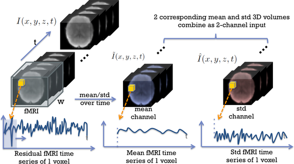
We start with preprocessed 3D fMRI volumes downsampled to 32 × 32 × 32. Since fMRI contains spatiotemporal information, it is intuitive to apply a sliding window along the time axis to capture the temporal information. We used sliding-windows with size w and stride length stride to move along the time dimension of the 4D fMRI sequence and calculated the mean and standard deviation (std) for each voxel’s time series within the sliding window. Thus, from each sliding window, a mean 3D image and std 3D image were generated with the same size as the downsampled fMRI 3D volume. Given T frames in each 4D fMRI sequence, by this method, $\lfloor \frac{T-w}{stride}\rfloor +1$ 2-channel images (mean and std fMRI images) were generated for each subject. Furthermore, the spatial information is preserved. We defined the original fMRI sequence as I(x, y, z, t), the mean-channel sequence as $\tilde{I}(x,y,z,t)$ and the std-channel as $\widehat{I}(x,y,z,t)$. For any x, y, z in {0, 1, ⋯, 31},

$$\tilde{I}(x,y,z,t)=\frac{{\sum }_{\tau =t+1-w}^{t}I(x,y,z,\tau )}{w}$$

$$\widehat{I}(x,y,z,t)=\sqrt{\frac{{\sum }_{\tau =t+1-w}^t{\left[I(x,y,z,\tau )-\tilde{I}(x,y,z,t)\right]}^2}{w-1}}.$$

This process is also described in Fig. 1.

Fig. 1.

Generating 2-channel input 3D images

2.2. 2CC3D Model

Tran et al.’s C3D convolutional architecture is well suited for 3D spatial feature learning [7]. For our purpose, a modified C3D model (number of kernels were changed and fewer layers were used) was trained to classify the preprocessed fMRI sliding window 2 channel images. The network architecture is shown in Fig. 2. It has 6 convolutional, 4 max-pooling and 2 fully connected layers, followed by a sigmoid output layer. The number of kernels and the layer types are denoted in each box. All 3D convolutional kernels were 3 × 3 × 3 with stride 1 in all dimensions. All the pooling kernels were 2 × 2 × 2. Binary cross entropy was used as the loss function. Dropout layers were added with ratio 0.5 after the first and the second max pooling layers and ratio 0.65 after the third and the fourth max pooling layers. L₂ regularization with regularisation 0.01 was used in each fully connected layer to avoid overfitting.

Fig. 2.

modified C3D architecture

2.3. Subject Classification by Majority Voting

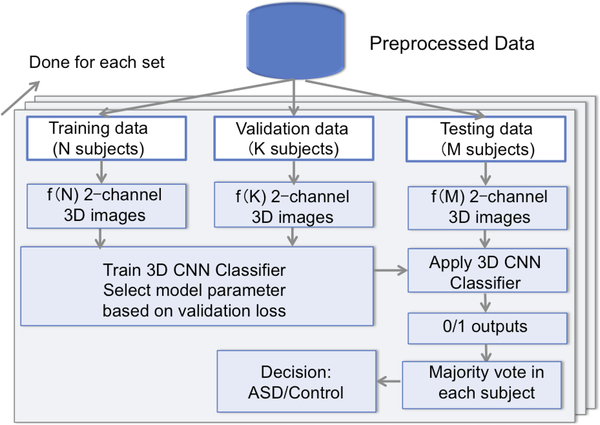
Each subject had $\lfloor \frac{T-w}{stride}\rfloor +1$ frames of 2-channel 3D images. During testing, each 2-channel 3D image was input into the trained neural network, resulting in a binary output. Thus for each subject, the output was a list of 0s or 1s, which had the same length as the total number of 2-channel image frames. The final decision of whether the subject was ASD or control was made by majority voting in the subject’s output list. The training and testing pipeline is illustrated in Fig. 3, where $f(n)=n\ast \left(\lfloor \frac{T-w}{stride}\rfloor +1\right)$.

Fig. 3.

Pipeline of training the CNN model and predicting classification results

2.4. Interpreting the Network

Characterizing ASD from fMRI and interpreting the features captured by the classifier can help neuroscientists better understand ASD. The 3D filters in the 2CC3D network capture spatial information in the 3D images. By exploring the output of the convolutional layers, we can find the salient regions activated by the proposed classifier’s filters.

3. EXPERIMENTS AND RESULTS

3.1. fMRI Acquisition and Preprocessing

We tested our methods on a group of 82 ASD children and 48 age-matched (p > 0.1) and IQ-matched (p > 0.1) healthy controls. Each subject underwent a T1-weighted scan (MPRAGE, TR = 1900ms, TE = 2.96ms, flip angle = 9°, voxel size = 1mm³ ) and a task fMRI scan (BOLD, TR = 2000ms, TE = 25ms, flip angle = 60°, voxel size = 3.44 × 3.44 × 4mm³, 164 volumes) acquired on a Siemens MAGNETOM Trio TIM 3T scanner.

For the fMRI scans, subjects viewed point light animations of coherent and scrambled biological motion in a block design [2] (24s per block). The fMRI data was preprocessed using FSL [8] as follows: 1) motion correction using MCFLIRT, 2) interleaved slice timing correction, 3) BET brain extraction, 4) spatial smoothing (FWHM=5mm), and 5) high-pass temporal filtering. The functional and anatomical data were registered to the MNI152 standard brain atlas [9]. The first few frames were discarded, resulting in 146 frames for each fMRI sequence.

3.2. Model Training and Testing

In our experiments, validation data was used to choose the best stopping epoch, avoiding overfitting. To test the robustness of the algorithm, four sets of training, validation and testing subjects were randomly sampled with stratification based on the subject’s label (control or ASD). For every set, 85% of the subjects were selected as training data, 7% of the subjects were selected as validation data, 8% of the subjects were selected as testing data. All the 3D volume data were standardized by subtracting the mean and dividing all voxels by the maximum absolute value before feeding into the model. In statistical analysis of binary classification, the F score is a measure of a test’s accuracy. It consider both $Precision=\frac{tp}{tp+fp}$ and $Recall=\frac{tp}{tp+fn}$, where tp is true positive, fp is false positive and fn is true negative. The F-score is defined as 2Precision Recall/(Precision + Recall). F-scores of each testing performance were recorded.

3.3. Input Comparison

Initially, the modified C3D network was tested on task fMRI and residual fMRI without sliding window. The task-fMRI did not perform well (Table 1) likely because the 3D volumes varied in a single subject, and it was difficult to learn the common features for all the 3D volumes in a single subject. Residual-fMRI is the signal that represents the residual after modeling out the biological and scrambled motion blocks and their temporal derivative effects from task-fMRI by GLM analysis [10]. Residual-fMRI is independent on the task parameters and subject parameters, making it easier to learn the common features of the fMRI signals in the same class. So our sliding window experiment was based on residual-fMRI. From each sliding window we generate a mean and a std image. Then the single mean channel input, single std channel input, and the combined 2-channel input were tested in the proposed 2CC3D model. Sliding window data were generated using w = 3 and stride = 1.

Table 1.

F-score of different inputs (w = 3, stride = 1)

Input	task-fMRI	residual-fMRI	std-channel	mean-channel	2-channel
F-score	0.70 ± 0.15	0.83 ± 0.06	0.78 ± 0.03	0.85 ± 0.07	0.89±0.05

The results are shown in Table 1. The 2-channel input improved the F-score over other input strategies as mean-channel smoothed the noisy signal and 2CC3D model can learn noise information from std-channel. If the std of the voxel was too high, then the 2CC3D model would suppress the effect of voxel’s mean value.

3.4. Sliding-window Size Investigation

The sliding window size affected the total data size and the measurement summary in the temporal dimension. Sliding-window sizes of 2,3,5,7, and 9 were tested to find the appropriate window size w in our study. The results are shown in Table 2. When w = 2, smoothing and noise measuring were weak, so F-score was low. W = 3 or 5 achieved good results and the F-scores were almost the same. When w > 5, the F-score decreased. If the sliding window size was too big, the data size would decrease and some signals were oversmoothed. If the sliding window size was too small, signals would under-smooth and would capture too much variance in the temporal dimension. There was a trade-off between the total amount of data, the measurement information richness and denoising level, which could be partially controlled by w.

Table 2.

F-score of sliding window size (Input = 2-channel, stride = 1)

Window size	2	3	5	7	9
F-score	0.82 ± 0.06	0.89±0.05	0.87 ± 0.09	0.84 ± 0.02	0.80 ± 0.04

3.5. Model Comparison

We compared our model with l₂ Regularized Logistic Regression, Support Vector Machine (SVM) and Random Forest (RF) classification methods. The input to the other machine learning models were flattened to a 1D vector. Each 2-channel 3D image had 2×32×32×32 = 65536 dimensions, which exceeded the capacity of the machine learning comparison models. We used principal component analysis (PCA) based dimensional reduction. The dimension-reduced vector accounted for more than 85% of the variance of the original vector for both channels with 70 components. We verified increasing the number of component would not significantly increase the variance percentage of the original vector. Then we concatenated the 2-channel vectors into one with dimension 140. In the alternative machine learning experiments, the same 2-channel data sets (w = 3, stride = 1) as in the 2CC3D model were used. The best parameters for each alternative machine learning model was selected by validation. The 2CC3D model outperformed the other 3 machine learning models as shown in Table 3, likely because it retained spatial information without flattening the 3D images.

Table 3.

F-score of different models (Input = 2-channel, w = 3, stride = 1)

Model	Logistic	SVM	RF	2CC3D
F-score	0.69±0.14	0.68±0.06	0.82±0.06	0.89±0.05

3.6. What Does the 2CC3D Model Learn?

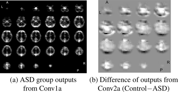
To characterize the features learned by the classifier, we looked at the output of the first two convolutional layers. There are 32 feature maps (32 × 32 × 32) from the first convolutional layer (Conv1a) and 64 feature maps (16×16×16) from the second convolutional layer (Conv2a). The output of each filter was averaged for 10 controls and for 10 ASDs. The 1st convolutional layer captured structural information and distinguished gray vs. white matter (shown in Fig. 4(a)). Its outputs are similar in both control and ASD group. The bright regions in Fig. 4(a) signifies strong filter activations, which highlight gray matter. The outputs of the 2nd convolutional layer showed significant differences between groups. The differences of the 2nd convolutional layer output between two groups (control−ASD) is shown in Fig. 4(b). The darker region denotes greater filter activation in the ASD group. Prefrontal cortex (motivation and emotion related) and cerebellum (cognition related) are very dark in Fig. 4(b); these regions have been linked to ASD by previous studies [2, 11]. The darkness in visual cortex could be caused by atypical visual perception of ASD subjects during the task, which was not modeled out in residual fMRI. ASD subjects may be looking at something else or even visually construing the stimuli differently than control subjects. Compared with group analysis of fMRI images [9], our 2CC3D model is a predictive method to learn ASD related biological markers for individual and new data.

Fig. 4.

Example outputs of 1 filter from the 1st conv layer and output difference between groups from 2nd conv layer. The slices were shown starting from the base of the brain.

4. SUMMARY

This paper proposed a new framework to classify ASD vs. control children using fMRI images. 2CC3D model used 3D convolutional neural networks to successfully handle high dimensional data and capture the spatial information. Using a sliding window approach, we generated enough data from limited subjects and reduced fMRI image noise. Experiments showed that our 2CC3D method using mean and std-channels as 3D CNN input outperformed the other models in our control vs. ASD fMRI classification case. Furthermore, middle layer outputs of the 2CC3D model showed promise for spatially identifying useful local information for classification. Future work will extend the proposed 2CC3D method on a public ASD dataset. In addition, we will explore more straightforward and interpretable ways of finding biological markers for ASD.