Low-dimensional dynamical characterization of human performance of cancer patients using motion data

Abstract

Background:

Biomechanical characterization of human performance with respect to fatigue and fitness is relevant in many settings, however is usually limited to either fully qualitative assessments or invasive methods which require a significant experimental setup consisting of numerous sensors, force plates, and motion detectors. Qualitative assessments are difficult to standardize due to their intrinsic subjective nature, on the other hand, invasive methods provide reliable metrics but are not feasible for large scale applications.

Methods:

Presented here is a dynamical toolset for detecting performance groups using a non-invasive system based on the Microsoft Kinect motion capture sensor, and a case study of 37 cancer patients performing two clinically monitored tasks before and after therapy regimens. Dynamical features are extracted from the motion time series data and evaluated based on their ability to i) cluster patients into coherent fitness groups using unsupervised learning algorithms and to ii) predict Eastern Cooperative Oncology Group performance status via supervised learning.

Findings:

The unsupervised patient clustering is comparable to clustering based on physician assigned Eastern Cooperative Oncology Group status in that they both have similar concordance with change in weight before and after therapy as well as unexpected hospitalizations throughout the study. The extracted dynamical features can predict physician, coordinator, and patient Eastern Cooperative Oncology Group status with an accuracy of approximately 80%.

Interpretation:

The non-invasive Microsoft Kinect sensor and the proposed dynamical toolset comprised of data preprocessing, feature extraction, dimensionality reduction, and machine learning offers a low-cost and general method for performance segregation and can complement existing qualitative clinical assessments.

1. Introduction

In oncologic practice, clinical assessments of performance stratify patients into subgroups and inform decisions about the intensity and timing of therapy as well as cohort selection for clinical trials. The Karnofsky performance status (KPS) (Karnofsky and Burchenal, 1948) and the ECOG/World Health Organization (WHO) performance status (Oken et al., 1982) are two equally prevalent measures of the impact of disease on a patient’s physical ability to function. The Karnofsky score is an 11-tier measure ranging from 0 (dead) to 100 (healthy) whereas the ECOG score is a simplified 6-tier score summarizing physical ability, activity, and self-care: 0 (fully active), 1 (ambulatory), 2 (no work activities), 3 (partially confined to bed), 4 (totally confined to bed), 5 (deceased) (Oken et al., 1982).

Although these metrics have been employed for many decades due the practicality, standardization of patient stratification, and speed of assessment, prospective studies have revealed inter- and intra-observer variability (Péus et al., 2013), gender discrepancies (Blagden et al., 2003), sources of subjectivity in physician assigned performance assessments (Péus et al., 2013), and a lack of standard conversion between the two different scales (Buccheri et al., 1996). Nevertheless performance status provides clinical utility because it is able to differentiate patient survival (Kawaguchi et al., 2010; Radzikowska et al., 2002). Consequently, the existing protocol of assigning a performance status based on an inherently subjective assessment must be refined to achieve a more objective classification of a patient’s physical function.

In contrast to the qualitative and relatively practical nature of physician assessments in the clinic, laboratory based invasive methods have been developed to biomechanically quantify elements of human performance. Many of these efforts have conducted gait analysis using accelerometer, gyroscope and other types of wearable sensors and motion capture systems (Tao et al., 2012) to detect and differentiate conditions in patients with osteoarthritis (Turcot et al., 2008), neuro-muscular disorders (Frigo and Crenna, 2009), and cerebral palsy (Desloovere et al., 2006). The shortcomings of more extensive assessments such as gait analysis include high cost, time required to perform tests, and general difficulty in interpreting results (Simon, 2004). The need for new technologies has been emphasized, particularly in the oncology setting (Kelly and Shahrokni, 2016), to bridge the gap between subjective prognostication using KPS or ECOG performance status and objective, yet cumbersome assessments of performance.

To this end, we propose a non-invasive motion-capture based performance assessment system which can (i) characterize performance groups using solely kinematic data and (ii) be trained to predict ECOG scores by learning from various physicians in order to reduce bias and intra-observer variability. The Microsoft Kinect is used as the motion-capture device due to its low cost, and ability to extract kinematic information without the need of invasive sensors. We describe and test a data processing and analysis pipeline using a cohort of 40 cancer patients who perform two clinically supervised tasks before and after therapy at USC Norris Comprehensive Cancer Center, Los Angeles County+USC Medical Center, and MD Anderson Cancer Center.

2. Methods

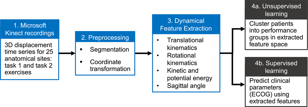
A set of dynamical analysis and machine learning tools is developed to gather kinematic information from recordings of patients performing tasks (Fig. 1) with the goal of validating the experiment design by performing unsupervised classification of performance categories (Fig. 1, step 4a), as well as supervised learning of physician assigned ECOG performance status (Fig. 1, step 4b). Although we illustrate the use of the toolset by exploring its application to an oncology cohort, the following methods are general and may be used to characterize patient performance in other settings.

Fig. 1.

Schematic of dynamical and machine learning analysis pipeline. Raw skeletal displacement data (step 1) from two clinically monitored tasks are preprocessed (step 2) before feature extraction (step 3) and two mutually exclusive machine learning analyses are performed. Unsupervised clustering (step 4a) of patients in a low dimensional space reveals the degree to which performance groups can by stratified using solely motion data. Supervised classification (step 4b) tests the ability of motion data to evaluate patients similar to physician ECOG performance status.

2.1. Experimental setup

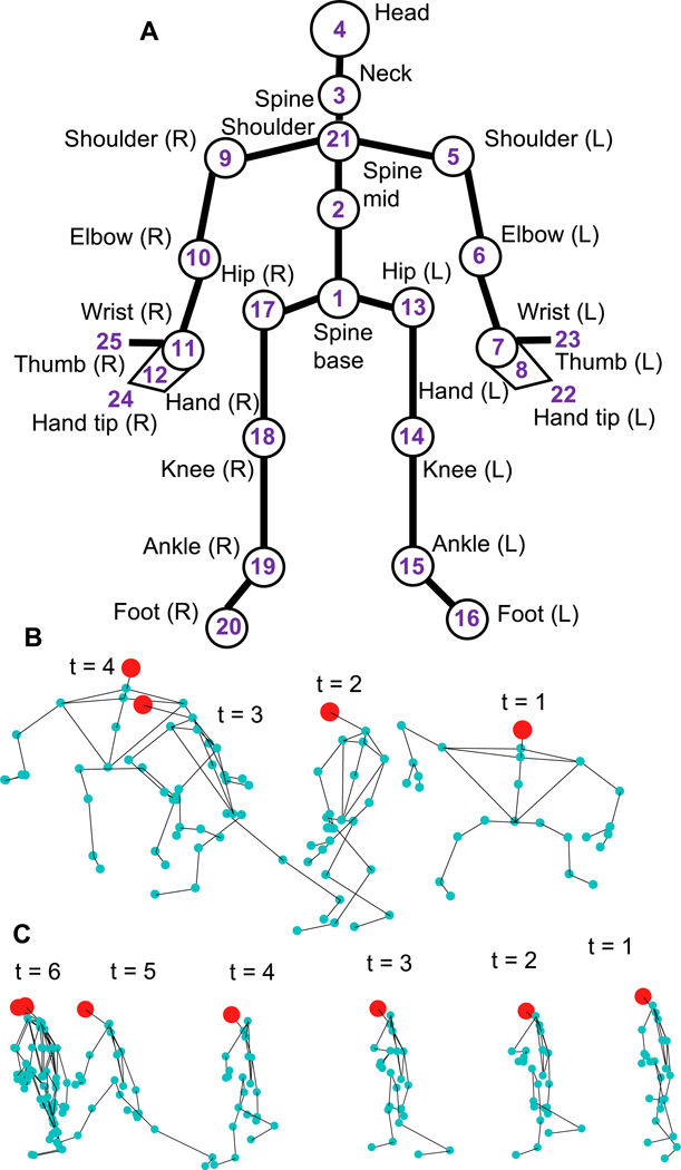
The Kinect depth sensor employs an infrared laser projector to detect a representative skeleton composed of 25 anatomical points (Fig. 2A) and recordings are post-processed using Microsoft Kinect SDK (v2.0) to extract 3-dimensional displacement time series data for the 25 points. The Microsoft Kinect sensor is used in the clinical setting to record patients performing two tasks: (i) task-1 requires patients, who start from a sitting a position, to stand up and sit down on an adjacent elevated medical table (Fig. 2B), (ii) task-2 requires patients to walk 8 ft towards the Kinect sensor, turn, and return to the original position (Fig. 2C). Both tasks are performed by each patient before and after a therapy cycle, providing two samples for each task for a total of four time series per patient. In both tasks the Kinect camera is secured to a tripod on a table, and oriented so as to capture the entire figure. Details about the data collection, skeletal data extraction, and experimental setup are described by Nguyen and Hasnain in Nguyen et al. (2017).

Fig. 2.

A) Kinect recordings are post-processed using Microsoft Kinect SDK (v2.0) to extract displacement time series data for a set of 25 anatomical joints and sites. B) Task-1 requires a patient to stand up from a chair and to sit at a medical table, a sample time series is shown. C) Task-2 sample time series, patient starts from a standing position (t = 1) and walks to a mark 8 ft away (t = 6) and returns to original position (not shown).

2.2. Data preprocessing

Due to irregularities in the positioning of the Kinect camera across different experiments, time series for task-2 is distorted such that a level plane (e.g. clinic floor) appears sloped in the recordings. To resolve this, an automated element rotation about the x-axis is performed. The angle of distortion θ ranges between 5 and 20° in the time series studied. The second preprocessing step involves manually segmenting the series to trim irrelevant data in the beginning and end of each task while the patient is stationary.

2.3. Feature extraction

The position vector, $\overrightarrow{r_i}(t)=\langle x_i(t),y_i(t),z_i(t)\rangle$ for an anatomical joint i is used to calculate its velocity magnitude,

$$v_i(t)=\Vert {\overrightarrow{\dot{r}}}_i(t)\Vert$$ (1)

and acceleration magnitude,

$$a_i(t)=\Vert {\overrightarrow{\ddot{r}}}_i(t)\Vert$$ (2)

using the mean-value theorem. In the absence of distribution of mass information, specific kinetic energy,

$$k{e}_i(t)=\frac{1}{2}{v}_i^2(t)$$ (3)

and specific potential energy,

$$p{e}_i(t)=g\text{Δ}{z}_i=g\left(z_i(t)-z_i(t=1)\right)$$ (4)

quantities are used to describe the energy signature of each anatomical joint. The sagittal angle, θ_s(t), is defined as the angle formed between the vector originating at the spine base and pointing in the direction of motion, and the vector connecting points 1 and 3 (Fig. 2A) at each time point t.

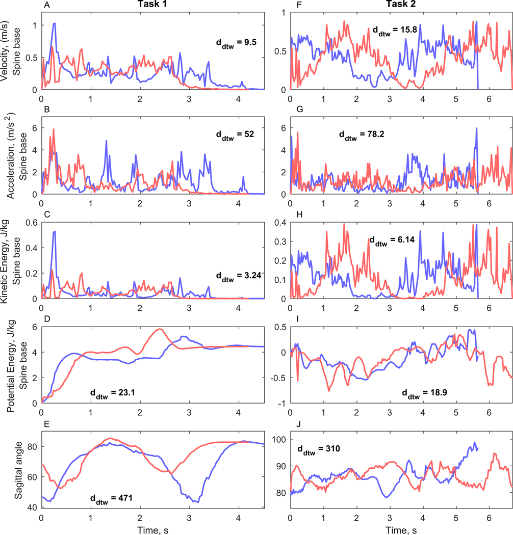
Time series corresponding to the hand (7, 8, 11, 12, 22, 23, 24, 25 in Fig. 2A) and feet (15, 16, 19, 20 in Fig. 2A) joints are relatively noisy therefore these time series are precluded from analysis, yielding 13 joints of interest in Fig. 2. In summary, the list of extracted features for each task performed by a patient during a single visit includes v_i, a_i, ke_i, pe_i, θ_s for i = 1,…,13 anatomical joints resulting in 53 time series features per task, and K = 106 time series features per visit (Fig. 4).

Fig. 4.

Example of extracted dynamical time series features (patient ID = 36). Before therapy (blue) and after therapy (red) feature time series are compared using DTW and the distances are annotated on the corresponding plots. A–E) Task-1 features. F–J) Task-2 features.

2.4. Time series similarity

For a given patient and task the before- and after-therapy time series of each feature are compared using a Euclidean metric dynamic time warping (DTW), which assigns a distance of zero for completely identical series and larger distances for more dissimilar series. Although DTW provides a distance which does not satisfy the triangle inequality and therefore is not a metric, it has been used extensively for time series clustering and classification (Ratanamahatana and Keogh, 2004). In the present work, DTW is used to describe changes in the extracted features where it is necessary to detect similar series despite noise and distortions which are intrinsic to the Kinect sensor and subsequent skeleton extraction. Consequently, the pair of before and after-therapy time series are assigned a DTW distance, d_DTW(p,k), for each patient p and feature k:

$$\mathbf{D}(p,k)=d_{DTW}(p,k)=\mathrm{DTW}\left(X_{1,k}^p,X_{2,k}^p\right)$$ (5)

where $X_{1,k}^p$ and $X_{2,k}^p$ are the time series of patient p’s feature k for visits 1 and 2 respectively. Calculating the DTW distance between before- and after-therapy visits for P patients and K features results in a matrix D ∈ℝ^P×K of DTW distances. This matrix captures the changes in the dynamical feature set before and after therapy. Feature distance vectors ${\overrightarrow{d}}_{k^{\prime }}\in {ℝ}^P$ for $k^{\prime }=1,\dots ,K$, whose entries are d_DTW(p,k′), are columns of D.

2.5. Dimensionality reduction

In practical applications, and the clinical case study presented here the number of patients who completed both visits, P = 37 ≪ K, therefore further dimensionality reduction is required before implementing learning algorithms based on the matrix D in order to avoid overfitting and the curse of dimensionality (Domingos, 2012). Here, we use principal component analysis (PCA) to recast D into a lower dimension space while still maintaining most of the variance in the data. The scale of DTW distances are feature dependent, therefore column-wise standardization of D is performed prior to PCA. This process results in a reduced distance matrix D_r ∈ℝ^P×N, comprised of N principal components, where N ≤ P.

2.6. Unsupervised clustering

Performance groups are detected in reduced principal component space by employing the K-medoids algorithm, where number of clusters, k, corresponds to the number of performance groups detected. The K-medoids algorithm is chosen as the unsupervised algorithm for its insensitivity to outliers and fast implementation for the small dataset studied.

The overall quality of the resulting clusters is assessed by varying (i) the number of clusters in the K-medoids algorithm, and (ii) the number of principal components N in the low dimensional distance matrix D_r and measuring the silhouette s of the resulting clusterings as well as the concordance between a given learned clustering and three clinical clusterings based on changes in weight before and after therapy,

$$\Delta \text{weight}={\text{weight}}_{\text{After therapy}}-{\text{weight}}_{\text{Before therapy}}$$ (6)

and change in ECOG performance status before and after therapy,

$$\Delta \text{ECOG}={\text{ECOG}}_{\text{After therapy}}-{\text{ECOG}}_{\text{Before therapy}}$$ (7)

and the number of unexpected hospital visits (UHV) where patients are grouped into 0, 1, and > 1 UHV over the course of the entire study. Changes in physician and coordinator assigned ECOG scores are used in this comparison.

The similarity between the ΔECOG, Δweight, UHV and Kinect based unsupervised clusterings is measured using the Rand index (RI):

$$RI\left(C,C^{\prime }\right)=\frac{a+b}{\left(\begin{array}{l}n\hfill \\ 2\hfill \end{array}\right)}$$ (8)

where C and C′ are two clusterings of n objects, a is the number of objects in the same clusters in C and C′, and b is the number of objects in separate clusters in C and C′. RI = 0 when there is complete disagreement between two clusterings, and RI = 1 for identical clusterings.

2.7. Supervised classification

Instead of comparing a given patient’s before- and after-therapy time series samples directly to each other as described in Section 2.4, a reference time series from a prototypical sample can be used to compare to the before- and after-therapy series separately. This approach allows for the construction of a distance matrix from a single patient visit, and enables subsequent machine learning models of the corresponding physician, coordinator, and patient assigned ECOG performance status. Three healthy subjects perform tasks 1 and 2 to generate the prototypical samples which serve as the reference points for patient performance, and DTW distances between a patient’s time series data and the prototypical samples offers a standardized measure of performance. The DTW distances to each of the L = 3 prototypical healthy samples are averaged for patient p’s extracted feature k from visit v, $X_{v,k}^p$,

$$d_{DTW}^v(p,k)=\frac{1}{L}\sum _{l=1}^L\mathrm{DTW}\left(X_{v,k}^p,X_k^l\right)$$ (9)

where $X_k^l$ is the l^th prototypical sample’s feature k, and visit v = 1 is the before-therapy sample and visit v = 2 is the after-therapy sample. Subsequently a standardized DTW distance matrix, D_s ∈ℝ^2P×K, is formulated in which each patient contributes a total of two rows for the two visits. D_s represents the task-1 and task-2 average DTW distance between a patient’s performance and the three prototypical samples. Along with a ℝ^2P vector of a ground-truth target variable, D_s can be used to develop supervised learning models. Here, we use the physician, coordinator, and patient assigned ECOG performance status as the target variables in three separate models.

3. Results & discussion

3.1. Current clinical parameters

37 patients completed the before and after therapy visits, and the corresponding physician and coordinator ECOG scores were recorded for a total of 74 visits, while only 31 patients reported ECOG scores (Table 1).

Table 1.

ECOG scores assigned to patients by physicians, coordinators, and patients themselves for the before and after therapy visits.

ECOG score distribution
	0	1	2	3	Total
Physician	35	37	2		74
Coordinator	37	35	2		74
Patient	19	27	9	2	57

For the subset of 57 cases of patient reported ECOG scores, from either one or both visits, the mutual information (MI) association between physician ECOG and patient ECOG scores is MI = 0.0653, while the association between coordinator ECOG and patient ECOG is MI = 0.1661. Consequently, there is a larger agreement between the coordinator and patient scores in the current experiment, however, more data needs to be collected to verify this trend.

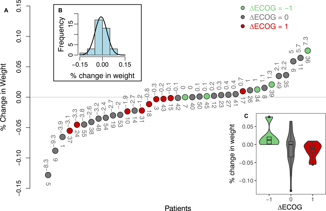
Fig. 3A shows the relationship between physician ΔECOG (Eq. (7)) and change in weight over therapy, where change in weight follows a normal distribution (Fig. 3B). However, due to the large spread of change in weight for ΔECOG = 0 group in Fig. 3C, there is no clear relation between ΔECOG and Δweight, suggesting either the patients are unhindered even when undergoing large weight change (e.g. patients 5, 9, 11 Fig. 3A) or that physicians consider other physical and expression cues more heavily while assigning ECOG scores.

Fig. 3.

A) Relation between change in physician assigned ECOG (Eq. (7)) and percent change in weight before and after therapy. The absolute change in weight in kg is annotated above the circles, and patient ID is annotated below. B) Histogram and normal distribution fit to percent change in weight. C) Boxplot of change in weight by ΔECOG groups.

Binning patients by the percent change in weight into groups of those who lose weight after therapy (Δweight < 2%), maintain weight (− 2% ≤Δweight ≤ 2%), and gain weight (Δweight > 2%) results in a weight based clustering of the patients, which has a RI = 0.509 (n = 37 patients) with the physician ΔECOG clustering. The UHV clusters are comprised of 16, 9, and 11 patients in the 0, 1, and > 1 UHV groups, and has a RI = 0.498 (n = 36) with the physician ΔECOG. Although the time points of the physician ECOG scores correspond to the before and after therapy visits, the UHV events are summed over the entire course of the study. The level of concordance between physician ECOG and existing clinical parameters serves as a benchmark for the unsupervised clustering in step 4a (Fig. 1).

3.2. Validation of preprocessing and choice of DTW

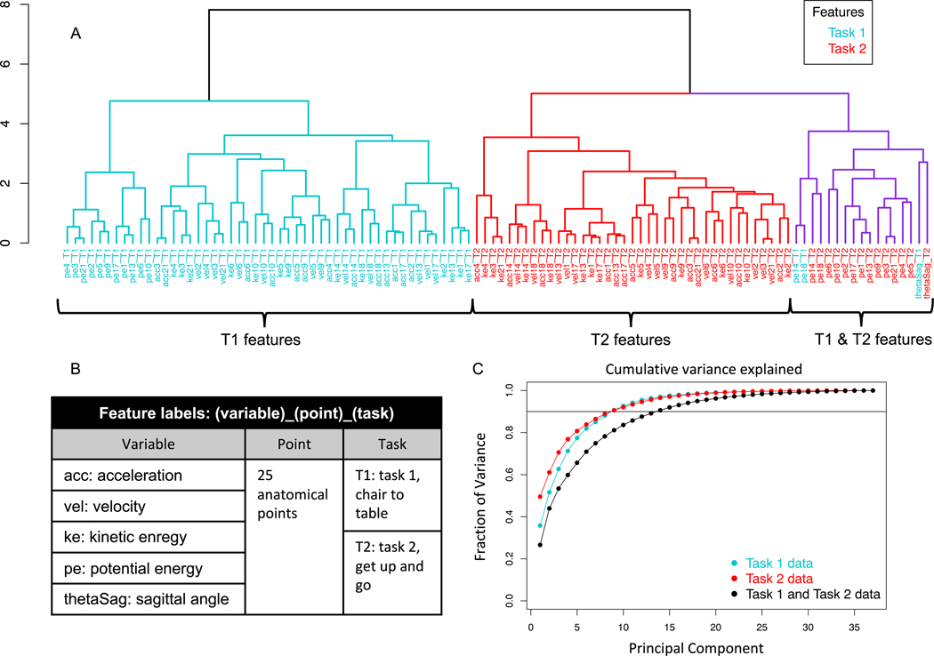
A hierarchical Euclidean distance based clustering of the task-1 and task-2 feature distances ${\overrightarrow{d}}_k{}^{\prime }$ (Fig. 5A, feature names in Fig. 5B) reveals that changes detected by DTW in most features are related mainly to other features of the same task, with the exception of a few features which correlate across tasks. These cross-task associated features include potential energies of the knee joints, and task 2 sagittal angle and left elbow potential energy to a lesser extent (purple, Fig. 5A). The smaller clusters within the larger task 1 (blue, Fig. 5A) and task 2 (red, Fig. 5A) clusters validate the preprocessing and DTW calculations of across-therapy time series feature because anatomically related sites appear in coherent subclusters. For instance the potential energy of the left and right hips (joints 13 and 17, Fig. 2A) and spine base (joint 1, Fig. 2A) appear in the same subclusters for both tasks respectively. Furthermore, the velocities for the knee joints 14 and 18 are more closely related in the task-2 subcluster than the task-1 subcluster, which makes sense intuitively because the knees synchronously oscillate while walking in task-2, but perform unique functions in the task-1 twisting motion of turning towards and climbing the medical table. Therefore, the choice of using DTW, despite its dependence on the underlying scale of the time series being compared, is suitable for the subsequent unsupervised and supervised learning analyses.

Fig. 5.

A) Hierarchical clustering dendrogram of task-1 and task-2 feature distance vectors ${\overrightarrow{d}}_k{}^{\prime }$. All but a few features (highlighted in purple) cluster primarily by task. B) Feature label nomenclature for the dendrogram in A. C) Fraction of variance explained by principal components of (i) distance matrix D comprised of task-1 and task-2 (K = 106) features (black), (ii) distance matrix D comprised of task-1 (K = 53) features (blue), and (iii) distance matrix D comprised of task-2 (K = 53) features (red).

3.3. Low dimension representation

The distance matrix D consisting of 106 feature distance vectors ${\overrightarrow{d}}_k{}^{\prime }$ (56 per task) shown in Fig. 5A constitutes a high dimensional representation of changes in the biomechanical performance of tasks 1 and 2 before and after therapy because the number patient samples is much less than the number of features: P = 37 ≪ K = 106.

A low dimension representation is achieved by performing PCA on distance matrices D consisting of task-1, task-2, and both task features to generate the reduced matrices D_r for comparison (Fig. 5C). In each case, a small number of reduced dimensions can explain a significant portion of the variance in the high-dimensional space. Specifically, reduced matrices for task-1 and task-2 each require 8 principal components to describe nearly 90% of variance in the corresponding high dimensional distance matrices. 13 principal components are required to capture a similar amount of variance when distance features from both tasks are included in D due to the relative lack of cross-task association between distance features shown in Fig. 5A. Nevertheless, the subsequent results are based on D which contains features from both tasks so as to prevent loss of information, and the additional task features do not adversely affect the learning algorithms.

The feature clustering and dimensionality reduction analyses in Fig. 5 illustrate the fact that both clinical tasks provide unique information and to use one test in the absence of the other would incur a loss of biomechanical information.

3.4. Detecting performance clusters

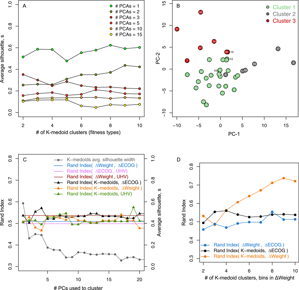
Changes in the before- and after-therapy performance of tasks 1 and 2 are captured in D_r, and the number of performance clusters detected in D_r is a latent variable derived by selecting the number of clusters, k, in the K-medoids clustering algorithm which minimizes the distance to a representative cluster patient, or medoid, in the reduced low-dimensional space spanned by the N principal components. Therefore the choice of the number of performance clusters, from strictly the machine learning perspective, is dependent on the balance between N and the corresponding quality of the clustering which is measured by the silhouette s ∈ [−1,1]. Higher values of s indicate higher intra-cluster cohesion and lower inter-cluster cohesion for a given patient. This balance is shown in Fig. 6, where greater number of dimensions in D_r generally correspond to lower average s. For instance, no matter the choice of k, a N = 2 distance matrix D_r cannot be clustered with a higher silhouette than a N = 1 distance matrix.

Fig. 6.

A) Quality of K-medoids patient clusterings measured by average silhouette s compared to the number of clusters k for different numbers of principal components N in the reduced distance matrix D_r. B) N = 3 and k = 3 K-medoids unsupervised clustering of patients shown in the plane formed by the first two principal components of D_r. C) The RI concordance between the k =3 K-medoids clusterings and physician ΔECOG (black), ΔWeight (yellow), and UHV (green) compared to benchmark RI associations among the ΔECOG, ΔWeight, and UHV based clusterings (solid lines). Quality of the K-medoids clusterings (gray) is shown on the right axis. D) Concordance between clusterings where the number of clusters in K-medoids and bins in ΔWeight are increased.

Here we seek the number of performance clusters to be much less than the number of patients in order to validate the unsupervised clustering with the three cluster Δweight, ΔECOG, and UHV clusterings, however, in general, larger values of k result in a higher resolution performance clustering of the patient group which in turn can be compared to higher resolution clinical categorizations.

From Fig. 6A, we select the N = k = 3 clustering and visualize it on the first two principal components in Fig. 6B, and compare all of the k = 3 clusterings to the physician ΔECOG, ΔWeight, and UHV clusterings in Fig. 6C. The number of principal components used in D_r to segregate patients in to k = 3 clusters is varied and the corresponding concordance, as measured by RI is shown on the left axis and the average silhouette on the right axis of Fig. 6C. Although the average silhouette of the K-medoid clusterings decreases with N, RI (K-medoid, ΔECOG), RI (K-medoid, ΔWeight), and RI (K-medoid, UHV) are maximized by N = 4, 17, and 19 principal components respectively.

As the number of principal components in the low-dimension space is varied, the concordance between the K-medoids clusters and the physician ΔECOG (black), ΔWeight (yellow), and the UHV (green) clusterings also changes (Fig. 6C). The K-medoids clustering has a higher RI with the ΔWeight clustering for most choices of N compared to the benchmark RI = 0.509 between physician ΔECOG and ΔWeight (Fig. 6C). As illustrated in Fig. 6C, the ΔECOG, ΔWeight, UHV, and the unsupervised clusterings all have a similar concordance, therefore, the distance matrix D of before- and after-therapy performance of task-1 and task-2 offers an objective platform to stratify patients, and, as shown by the RI metric, may achieve concordance with existing clinical measurements.

The RI between the unsupervised K-medoid clusterings and the clinical clusterings including the physician and coordinator assigned ΔECOG clusterings is shown in Table 2. The K-medoid clustering has the highest RI with the UHV clusters, and the second highest association with the ΔWeight. The coordinator ΔECOG clusters are more associated with the ΔWeight and UHV clusters than the physician ΔECOG clusters. Although these trends are particularly interesting, larger datasets are required to validate these RI values and to fully detect statistically significant disparities. Nevertheless, Table 2 shows that the K-medoid unsupervised clusterings based on kinematic changes in task-1 and task-2 across therapy offers a unique but useful patient clustering.

Table 2.

Association between patient clusterings based on the following: 1) unsupervised K-medoids clustering (k =3 clusters) of D_r, 2) ΔWeight: change in weight before and after therapy, 3) UHV: three clusters based on 0, 1, and > 1 unexpected hospital visits over the course of the study, 4) ΔECOG_P: change in physician ECOG scores before and after therapy, and 5) ΔECOG_C: change in coordinator ECOG scores before and after therapy.

Rand index between clusterings
	K-medoids	ΔWeight	UHV	ΔECOGP
ΔWeight	0.541
UHV	0.575	0.537
Δ ECOG P	0.571	0.509	0.498
Δ ECOG C	0.550	0.571	0.530	0.497

The added utility of the motion analysis based unsupervised clustering method shown here is the ability to achieve higher resolution clusterings of patients compared to physician or coordinator ΔECOG by increasing k in the K-medoids algorithm. Fig. 6D shows a comparison between N = 3 K-medoids and ΔWeight clusterings where k and the number of bins in the ΔWeight clustering are increased which leads to an increasing RI between the two clusterings and a maximum RI = 0.737 is reached at k = 9 clusters. This further demonstrates the potential clinical utility of the pipeline of analytical tools developed.

3.5. Learning physician ECOG performance status

A natural application of the Kinect motion capture system is to use the extracted kinematic signature of a patient’s task-1 and task-2 performance to learn the associated physician, coordinator, and patient assigned ECOG performance status, particularly if patients are examined by different physicians in order to reduce bias of the resulting model.

To learn the ECOG scores in the cancer patient cohort, we use the standardized distance matrix D_s (Section 2.7) and perform dimensionality reduction via PCA with scaling and centering. As in the unsupervised model, dimensionality reduction is required due to the relatively small number of patients compared to the number of features.

In the 74 physician and coordinator assessments of the P = 37 patients there are 2 ECOG = 2 cases. Since the majority of cases were ECOG = 0 or 1 scores, the two ECOG = 2 samples are excluded, and a binary classifier is trained to predict a 0 or 1 ECOG status using the two visits from P = 37 patients (excluding two ECOG = 2 cases from two separate patients), which results in a distance matrix for the physician and coordinator ECOG classifiers. For the patient classifier a D_s ∈ℝ^57×106 matrix is used and the ECOG = 1,2, and 3 categories are combined due to limited data.

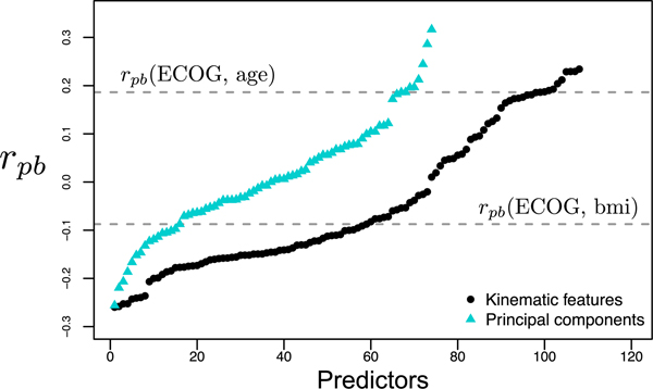
The association of the original features of D_s and its principal components with the ECOG status is measured by the point biserial correlation coefficient r_pb, where positive r_pb values indicate larger values of the feature are associated with ECOG = 1, and vice versa (Fig. 7).

Fig. 7.

Point biserial correlation between physician assigned ECOG and kinematic features of D_s (black) and reduced space principal components of D_s (blue). Larger r_pb values indicate association with ECOG = 1, and vice versa. The correlations of age and BMI with ECOG (gray dashed lines) serve as a comparison for the r_pb of the kinematic features and principal components.

For the physician ECOG, age has a r_pb = 0.186, as older patients were more likely to receive higher ECOG scores and in comparison, 10 principal components in the reduced D_s have a higher absolute r_pb. Principal components with the largest ||r_pb|| are used to create and cross-validate classifiers by leaving one patient’s two samples out as the test set. 10 principal components are used in a mixture-of-experts model comprised of a SVM, logistic regression, and a KNN model to predict physician ECOG with an average cross-validated test set accuracy of 84.7% accuracy. The same accuracy was achieved using the same number of principal components to predict coordinator ECOG with a SVM model. Top 5 principal components were used to train a logistic regression model to predict patient ECOG = 0 or > 0 which performed at an accuracy of 80.7%.

4. Conclusions

A non-invasive motion capture system is proposed to measure the kinematic signature of clinically supervised patient assessments of performance. A toolset to pre-process and extract dynamical features from skeletal displacement data is combined with complimentary unsupervised and supervised learning schemes. The unsupervised clusters reveal a new and valuable grouping of patients in a cancer cohort undergoing therapy. Additionally, the supervised learning model is able to predict physician, coordinator, and patient assigned ECOG scores using the kinematic signature with a high level of accuracy. In comparison to the low-resolution ECOG scale, the present toolset provides a pipeline to develop a high resolution performance grading. In general, the dynamical characterization toolset may be used for prognostication in various applications where biomechanical signatures are reasonably correlated with existing clinical measures. The present work is a proof of concept of a low-cost non-invasive method for objectively assessing human performance in the clinic.

References

- Blagden S, Charman S, Sharples L, Magee L, Gilligan D, 2003. Performance status score: do patients and their oncologists agree? Br. J. Cancer 89 (6), 1022. [DOI] [PMC free article] [PubMed] [Google Scholar]
- Buccheri G, Ferrigno D, Tamburini M, 1996. Karnofsky and ECOG performance status scoring in lung cancer: a prospective, longitudinal study of 536 patients from a single institution. Eur. J. Cancer 32 (7), 1135–1141. [DOI] [PubMed] [Google Scholar]
- Desloovere K, Molenaers G, Feys H, Huenaerts C, Callewaert B, Van de Walle P, 2006. Do dynamic and static clinical measurements correlate with gait analysis parameters in children with cerebral palsy? Gait Posture 24 (3), 302–313. [DOI] [PubMed] [Google Scholar]
- Domingos P, 2012. A few useful things to know about machine learning. Commun. ACM 55 (10), 78–87. [Google Scholar]
- Frigo C, Crenna P, 2009. Multichannel SEMG in clinical gait analysis: a review and state-of-the-art. Clin. Biomech 24 (3), 236–245. [DOI] [PubMed] [Google Scholar]
- Karnofsky D, Burchenal J, 1948. The evaluation of chemotherapeutic agents against neoplastic disease In: Cancer Research. vol. 8 Amer Assoc Cancer Research PO Box 11806, Birmingham, AL: 35202, pp. 388–389. [Google Scholar]
- Kawaguchi T, Takada M, Kubo A, Matsumura A, Fukai S, Tamura A, Saito R, Maruyama Y, Kawahara M, Ou S-HI, 2010. Performance status and smoking status are independent favorable prognostic factors for survival in non-small cell lung cancer: a comprehensive analysis of 26,957 patients with NSCLC. J. Thorac. Oncol 5 (5), 620–630. [DOI] [PubMed] [Google Scholar]
- Kelly CM, Shahrokni A, 2016. Moving beyond Karnofsky and ECOG performance status assessments with new technologies. J. Oncol 2016. [DOI] [PMC free article] [PubMed] [Google Scholar]
- Nguyen MNB, Hasnain Z, Li M, Dorff T, Quinn D, Purushotham S, Nocera L, Newton PK, Kuhn P, Nieva J, Shahabi C, 2017. Mining human mobility to quantify performance status. In: 2017 IEEE International Conference on Data Mining Workshops (ICDMW), pp. 1172–1177. 10.1109/ICDMW.2017.168. [DOI] [Google Scholar]
- Oken MM, Creech RH, Tormey DC, Horton J, Davis TE, McFadden ET, Carbone PP, 1982. Toxicity and response criteria of the eastern cooperative oncology group. Am. J. Clin. Oncol 5 (6), 649–656. [PubMed] [Google Scholar]
- Péus D, Newcomb N, Hofer S, 2013. Appraisal of the Karnofsky performance status and proposal of a simple algorithmic system for its evaluation. BMC Med. Inform. Decis. Mak. 13 (1), 72. [DOI] [PMC free article] [PubMed] [Google Scholar]
- Radzikowska E, Głaz P, Roszkowski K, 2002. Lung cancer in women: age, smoking, histology, performance status, stage, initial treatment and survival. population-based study of 20 561 cases. Ann. Oncol 13 (7), 1087–1093. [DOI] [PubMed] [Google Scholar]
- Ratanamahatana CA, Keogh E, 2004. Everything you know about dynamic time warping is wrong. In: Third Workshop on Mining Temporal and Sequential Data Citeseer, pp. 22–25. [Google Scholar]
- Simon SR, 2004. Quantification of human motion: gait analysisbenefits and limitations to its application to clinical problems. J. Biomech 37 (12), 1869–1880. [DOI] [PubMed] [Google Scholar]
- Tao W, Liu T, Zheng R, Feng H, 2012. Gait analysis using wearable sensors. Sensors 12 (2), 2255–2283. [DOI] [PMC free article] [PubMed] [Google Scholar]
- Turcot K, Aissaoui R, Boivin K, Pelletier M, Hagemeister N, de Guise JA, 2008. New accelerometric method to discriminate between asymptomatic subjects and patients with medial knee osteoarthritis during 3-d gait. IEEE Trans. Biomed. Eng. 55 (4), 1415–1422. [DOI] [PubMed] [Google Scholar]