Modelling and control of a fractional-order epidemic model with fear effect

Abstract

In this paper, we formulate and study a new fractional-order SIS epidemic model with fear effect of an infectious disease and treatment control. The existence and uniqueness, nonnegativity and finiteness of the system solutions for the proposed model have been analysed. All equilibria of the model system are found, and their local and also global stability analyses are examined. Conditions for fractional backward and fractional Hopf bifurcation are also analysed. We study how the disease control parameter, level of fear and fractional order play a role in the stability of equilibria and Hopf bifurcation. Further, we have established our analytical results through several numerical simulations.

Introduction

Infectious diseases have become one of the most threatening issues in todays lifestyle. The infectious diseases including chickenpox, measles, cholera, tuberculosis, influenza, SARS, COVID-19, etc., have massive impact than the other types of noninfectious diseases as these types of diseases can be transmitted from one individual to another, some are spread out by bites from insects or animals, and some diseases are acquired by consuming flagitious water or food or being exposed to organisms in the environment. Hence, an infectious disease may spread in a huge region throughout the globe within a very short time period. Due to the improvement of lifestyle of common people and massive enhancement in transportation and globalization, an infectious diseases become pandemic in a less amount of time compared to earlier days (for example Spanish flu in twentieth century had taken a long period of time to become a pandemic compared to the pandemic due to COVID-19 in ongoing time period). Thus, not only to study the dynamics of an infectious disease, but also to control or determining the procedure to control an infectious disease, researchers from various fields have engaged themselves.

Several mathematical tools induce a great affect in regulating many infectious diseases. Mathematical modelling is one of the popular and commonly used mathematical tools that can be utilized efficaciously to monitor several infectious diseases. The first effective research work on studying an infectious diseases using mathematical model was probably first done by Kermack and Mckendric (1927). There are several research works where the authors have been studied mathematical models on controlling infectious diseases (see Zhou et al. 2014; Jana et al. 2016, 2017a). In his book, Murray (2002) has analysed theoretical works on some simple SI,  SIS,  SIR epidemic models. Present days mathematicians formulate more complex epidemic model systems which are almost identical to the real-world problems. In mathematical studies of an epidemic model, proper control strategies are significant tools in monitoring and controlling the infectious diseases. In this regard, two most effective and commonly used control tools used in controlling diseases are vaccination and treatment (Kar and Jana 2013a, b). However, isolation (see Jana et al. 2017b), insecticide (to control vector-borne disease)(see Kar and Jana 2013b), etc., are also used in recent days.

In the present work, we consider fear factor due to the infectious disease which is an another important parameter for epidemic model. People generally got scared and make a significant distance to prevent the infectious disease. Hence, fear induced by the infectious disease compelled susceptible population to isolate which actually decreases the birth rate of population and also survival of adults is affected consequently. Due to the SARS outbreak in HongKong (SARS started on November 2002; peaked on March 2003; eliminated on June, 2003), the birth rate dramatically had fallen from 8.742 (2002) to 8.436 (2003) and again it increased to 8.558 in 2004 (see Worldbank (2018)). In our work, we formulate a new fractional-order SIS epidemic model with fear effect (Clinchy et al. 2013; Wang et al. 2016) and treatment control to eradicate the disease.

Mathematical models based on ordinary differential equations depict the interactions between the population classes (e.g. susceptible-infected), and it is a classical approach in theoretical epidemiology. In recent days, researchers are concerned in developing mathematical model by the fractional-order differential equations because it is an important apparatus for the study of the memory and also some hereditary properties of several biological components and also it has a very close relation to the fractal theory. These are the main advantages of the fractional-order derivatives which are not included in the models based on the ordinary-order derivatives. Therefore, fractional-order derivatives are more naturalistic than the ordinary derivatives. The models constructed by the fractional-order derivatives have been widely applied in different field of research after the some famous books and research works on fractional-order differential equations (Diethelm and Braunschweig 2003; Hilfer 2000; Kilbas et al. 2006; Miller and Ross 1993; Petras 2011; Podlubny 1999; Sabatier et al. 2007; Sengupta et al. 2020; Yadav et al. 2020; Karthikeyan and Arul 2020). However, a fractional-order derivative may be defined in several ways. The most popular and commonly useful definitions of fractional-order derivatives are in the sense of Riemann–Liouville, Grünwald–Letnikov and Caputo definitions (Petras 2011; Podlubny 1999). Since, in the definition due to Caputo, the initial conditions can be expressed in a similar fashion as the integer-order differentiation, it is the most frequently used fractional-order derivative in mathematical modelling. There are very few theories to analyse the dynamical behaviour of the mathematical models with fractional-order derivatives (Delavari et al. 2012; Deshpande et al. 2017; Guo 2014; Li et al. 2016; Liang and Wu 2015; Li et al. 2010). In recent days, the linearization, Lyapunov method and Lyapunov direct method (due to Lyapunov function Garrappa 2010) have established to study the local and global stability of equilibrium point(s) of a fractional-order system.

Our research article studies the modelling and control of an epidemic problem using some advanced mathematical tools. In particular, this article focuses on approaches that integrate ecology and environment considerations and promote multidisciplinary solutions for tackling environmental problems and complex socio-economic problems. Present global scenarios show that human epidemiology has a significant impact on both the ecology and the environment. As this research article studies the modelling and control of an epidemic problem, the theoretical analysis of epidemiology is relevant to both ecology and environment (see Venturino et al. 2016; Maji et al. 2019; Khatua et al. 2020, etc.). Moreover, the modelling approach using fractional-order differential equations gives an additional novelty and dimension of the article.

The rest of the article is prepared as follows: in Sect. 2, we formulate an SIS-type fractional-order epidemic system and then discuss some preliminaries on fractional-order derivatives in Sect. 3. In Sect. 4, we describe the dynamics of the proposed model, including equilibria, their existence, bifurcation and both the local and the global behaviours. In Sect. 5, we present some computer simulation works to validate our theoretical observations. In Sect. 6, we provide some of the central findings of the paper and the last section is devoted to draw the conclusions of the paper.

Model formulation

In this section, we construct a new fractional-order SIS (susceptible-infected-susceptible)-type epidemic model with treatment control and fear effect due to the infectious disease. We separate the total populations into two time-dependable mutually exclusive classes, viz. susceptible S(t) (vulnerable for the infectious disease) and infected I(t) (already have pathogen of the disease and infectious for the population). Assume that birth rate of the susceptible population be r, natural death rate of both susceptible and infected population be a and d be the death rate due to the disease. Also, consider b as the death rate of susceptible population due to intraspecific competition (Ghirlanda et al. 2009). Note that b is smaller as compared to a, but it is not negligible for a large population. Further, let us take fear function as $f(\beta ,I)$ which reduces the growth rate of susceptible population. Again, we consider that the disease transmission function is g(I) and the disease control function is h(u). Consider m as the natural recovery rate of the infected population from the disease. Finally, assume that the recovery from infectious disease is not permanent and hence all the recovered individuals will be reinfected, i.e. they are susceptible to the infectious disease. We formulate our proposed model in the following form by the above conditions:

$$\begin{array}{c}\hfill \begin{array}{cc}\hfill {}_{t_0}{D}_t^{\alpha }S(t)& =rf(\beta ,I)S-aS-b{S}^2-g(I)S+[m+h(u)]I\hfill \\ \hfill {}_{t_0}{D}_t^{\alpha }I(t)& =g(I)S-[m+h(u)]I-(a+d)I\hfill \\ \hfill \end{array}\end{array}$$ 2.1

Here ${}_{t_0}{D}_t^{\alpha },\alpha \in (0,1]$ is the fractional-order derivative ($\alpha$-order) in the sense of Caputo (Petras 2011; Podlubny 1999). In our present model, we consider fear function as $f(\beta ,I)=\frac{1}{1+\beta I}$ with the level of fear as $\beta$ and the disease transmission function as $g(I)=\frac{\gamma I}{1+\delta I}$, where $\gamma$ is disease transmission rate and $\delta$ is half-saturation incidence rate. Further, we assume that the disease control function is $h(u)=u$. Here u is the treatment control. So our model becomes

$$\begin{array}{c}\hfill \begin{array}{cc}\hfill {}_{t_0}{D}_t^{\alpha }S(t)& =\frac{\mathit{rS}}{1+\beta I}-aS-b{S}^2-\frac{\gamma SI}{1+\delta I}+(m+u)I\hfill \\ \hfill {}_{t_0}{D}_t^{\alpha }I(t)& =\frac{\gamma SI}{1+\delta I}-(m+u)I-(a+d)I\hfill \\ \hfill \end{array}\end{array}$$ 2.2

System (2.2) for different fractional differentiations ${\alpha }_1,{\alpha }_2\in (0,1]$ is known as incommensurate fractional-order system. It is presented by following way

$$\begin{array}{c}\hfill \begin{array}{cc}\hfill {}_{t_0}{D}_t^{{\alpha }_1}S(t)& =\frac{\mathit{rS}}{1+\beta I}-aS-b{S}^2-\frac{\gamma SI}{1+\delta I}+(m+u)I\hfill \\ \hfill {}_{t_0}{D}_t^{{\alpha }_2}I(t)& =\frac{\gamma SI}{1+\delta I}-(m+u)I-(a+d)I\hfill \\ \hfill \end{array}\end{array}$$ 2.3

System (2.2) is known as commensurate fractional-order system. Note that all the parameters considered in the formulations of the model are nonnegative.

Some preliminaries

In this section, we recall some essential definitions, effective lemmas for both types of commensurate and incommensurate fractional-order systems.

Definition 3.1

(Petras 2011) The Caputo-type fractional-order derivative of $\alpha >0$ order for the function $f:C^n[t_0,\infty )\to \mathbb{R}$ may be defined and denoted by:

$$\begin{array}{c}\hfill {}_{t_0}{D}_t^{\alpha }f(t)=\frac{1}{\Gamma (n-\alpha )}{\int }_{t_0}^t\frac{f^{(n)}(\zeta )}{{(t-\zeta )}^{\alpha -n+1}}d\zeta \end{array}$$

where $C^n[t_0,\infty )$ is a space of n times continuously differentiable functions on $[t_0,\infty )$, $t>t_0$ and $\Gamma (·)$ be the Gamma function with $n\in {\mathbb{Z}}^{+}$ (the set of all positive integers) such that $n-1<\alpha <n$. Particularly, if $0<\alpha <1$, the definition becomes:

$$\begin{array}{c}\hfill {}_{t_0}{D}_t^{\alpha }f(t)=\frac{1}{\Gamma (1-\alpha )}{\int }_{t_0}^t\frac{f^{\prime }(\zeta )}{{(t-\zeta )}^{\alpha }}\mathrm{d}\zeta \end{array}$$

Lemma 3.2

(Odibat and Shawagfeh 2007) Let us assume that $\alpha \in (0,1]$and both the functions f(t) and its fractional derivative ${}_{t_0}{D}_t^{\alpha }f(t)$be elements of the metric space C[a, b] . If ${}_{t_0}{D}_t^{\alpha }f(t)\ge 0$then the function f(t) is a monotone increasing, and the function is monotone decreasing if ${}_{t_0}{D}_t^{\alpha }f(t)\le 0$for all $t\in [a,b]$.

Lemma 3.3

(Li et al. 2016) Let us consider that $x:[t_0,\infty )\to \mathbb{R}$be continuous function and satisfies the following:

$$\begin{array}{cc}& {}_{t_0}{D}_t^{\alpha }x(t)+\mu x(t)\le \nu ,x(t_0)=x_0,t_0\ge 0,\mu ,\nu \in \mathbb{R},\hfill \\ \hfill & \mu \ne 0,\mathrm{and}\alpha \in (0,1)\hfill \end{array}$$

Then we have the inequality:

$$\begin{array}{c}\hfill x(t)\le \left(x_0,-,\frac{\nu }{\mu }\right)E_{\alpha }[-\mu {(t-t_0)}^{\alpha }]+\frac{\nu }{\mu }\end{array}$$

for all $t\ge t_0$. Here $E_{\alpha }$is the Mittag–Leffler function of one parameter.

Lemma 3.4

(Petras 2011) Assume the following fractional-order system of the order $\alpha \in (0,1]$

$$\begin{array}{c}\hfill {}_{t_0}{D}_t^{\alpha }x(t)=Mx,x(t_0)=x_0>0.\end{array}$$

where $x\in {\mathbb{R}}^n$and $M\in {\mathbb{R}}^{n\times n}$ (set of all n × n real matrices). The system is said to be stable asymptotically iff $|arg(\lambda )|>\frac{\alpha \pi }{2}$satisfy for each of the eigenvalues $\lambda$of the matrix M and the system is said to be stable only iff $|arg(\lambda )|\ge \frac{\alpha \pi }{2}$for each of the eigenvalues of matrix M with the eigenvalues satisfying the critical condition $|arg(\lambda )|=\frac{\alpha \pi }{2}$must have geometric multiplicity one.

Lemma 3.5

(Petras 2011) Let us assume the fractional-order system of the order $\alpha \in (0,1]$

$$\begin{array}{c}\hfill {}_{t_0}{D}_t^{\alpha }x(t)=f(x),x(t_0)=x_0>0\end{array}$$

where $x\in {\mathbb{R}}^n$. A stationary point of the system is called to be locally asymptotically stable iff $|arg({\lambda }_k)|>\frac{\alpha \pi }{2}$for all eigenvalues ${\lambda }_k(k=1,2\dots n)$of Jacobian matrix $J=\frac{\partial f}{\partial x}$calculated at the corresponding stationary point.

The fractional-order system

Here, first we assume commensurate fractional-order system (2.2) by considering ${\alpha }_1={\alpha }_2=\alpha \in (0,1]$ in the incommensurate system (2.3).

Equilibria

Now we analyse the existence criteria of nonnegative equilibria of constructed system (2.2). The system possesses the equilibrium points which are trivial equilibrium (TE) $E^0(0,0)$, disease-free equilibrium (DFE) $E^1((r-a)/b,0)$ and three endemic equilibria (EE) $E^{\ast }(S^{\ast },I^{\ast })$, $E_1^{\ast }(S_1^{\ast },I_1^{\ast })$ and $E_2^{\ast }(S_2^{\ast },I_2^{\ast })$ depending upon the positive roots $I^{\ast }$, $I_1^{\ast }$ and $I_2^{\ast }$ of the following cubic equation.

$$\begin{array}{c}\hfill a_0{I}^3+a_1{I}^2+a_{2}I+a_3=0\end{array}$$ 4.1

where $a_0=b\beta {\delta }^2{(a+d+m+u)}^2$,

• $a_1=b\delta (2\beta +\delta ){(a+d+m+u)}^2+\beta \gamma [(a+\gamma )(a+d)+a\delta (m+u)]$,

• $a_2={\gamma }^2(a+d)+(a+d+m+u)\{b(\beta +2\delta )(a+d+m+u)+\gamma [a\beta +\delta (a-r)]\}$ and

• $a_3=b(a+d+m+u)\{b(a+d+m+u)+\gamma a\}(1-R_0)$,

where $R_0=\frac{\gamma r}{b(a+d+m+u)+\gamma a}$ is known as the basic reproduction number which can be defined as the number of new infections made by an infected individual to the susceptible population during its infection period. Also, $S^{\ast }=\frac{(1+\delta I^{\ast })(a+d+u)}{\gamma }$, $S_1^{\ast }=\frac{(1+\delta I_1^{\ast })(a+d+u)}{\gamma }$ and $S_2^{\ast }=\frac{(1+\delta I_2^{\ast })(a+d+u)}{\gamma }$.

We rewrite the cubic equation (4.1) in following standard form of strum’s function

$$\begin{array}{c}\hfill x^3+3Ax+B=0\end{array}$$ 4.2

where $x=a_{0}I+\frac{a_1}{3}$, $A=\frac{3a_0{a}_2-a_1^2}{9}$ and $B=\frac{27a_0^2{a}_3-9a_0{a}_1{a}_2+2a_1^3}{27}.$

The strum’s functions of equation (4.2) may be represented as

$$\begin{array}{cc}\hfill f(x)=& x^3+3Ax+B,f_1(x)=x^2+A,\hfill \\ \hfill f_2(x)=& -2Ax-B,\text{and}{f}_3(x)=-(B^2+4A^3).\hfill \end{array}$$

We use the famous Strum’s theorem to verify the existence of number of distinct positive roots of equation (4.2) and hence of equation (4.1). It can be easily verified that $B^2+4A^3<0$ implies equation (4.2) possesses three distinct real roots. The condition $B^2+4A^3<0$ implies that $A<0$. See that if $a_2<0$, then $A<0$. Now $f(\infty )>0,f_j(\infty )>0,j=1,2,3$. Here the number of changes of signs of the successive strum’s functions is zero. Again $f(0)=B,f_1(0)=A<0,f_2(0)=-B,f_3(0)=-(B^2+4A^3)>0$. Here the number of changes of signs of the strum’s functions depends on the sign of B. If $B<0$, then the number of changes sign of the successive strum’s functions is one, and hence equation (4.2) possesses exactly one positive root. If $B>0$, then the number of changes sign of the successive strum’s functions is two, and hence equation (4.2) possesses exactly two positive roots. Since $a_0,a_1>0$ for any choice of parameters, $a_3<0,a_2>0$ and $2a_1^2<9a_0{a}_2$ together imply that $B<0$. Now $a_3<0$ implies that $R_0>1$ and $a_2>0$ implies that $a>r$. Again $a_3>0,a_2<0$ together imply that $B>0$. Now $a_3>0$ implies that $R_0<1$. With this above discussion, we state the next theorem:

Theorem 4.1

• (i)Proposed model system (2.2) possesses at least one EE if $R_0>1$.
• (ii)Proposed model system (2.2) possesses exactly two EE points if $R_0<1$and $a_2<0$. Otherwise, system (2.2) possesses unique EE if $B^2+4A^3<0$, $R_0<1$, $a>r$and $2a_1^2<9a_0{a}_2$.
• (iii)System (2.2) possesses no EE point if $R_0<1$and $a>r$.

From above Theorem 4.1, we can detect that system (2.2) possesses two endemic equilibrium points if $R_0<1$, the basic reproduction number is less than unity, and this confirms that the system passes through a backward bifurcation at $R_0=1$. Hence $R_0<1$ is not a sufficient condition to eradicate the disease from our system (Fig. 1).

Fig. 1.

Curve for backward bifurcation of model (2.2)

The backward bifurcation diagram shows that when $R_0<1$, there exist two endemic equilibrium points and one of which is asymptotically stable and other is unstable.

Theorem 4.2

(El-Saka 2015) Fractional-order system (2.2) undergoes backward bifurcation at $R_0=1$iff $a_2<0$and $a_3(\beta )=0$.

Here we choose $\beta$ as backward bifurcation parameter. If the condition (ii) of Theorem 4.1 is true (the conditions for the existence of two EE points), then system (2.2) possesses backward bifurcation at $R_0=1$. This implies that system (2.2) goes through two EE points in the interval $[R_0^{\ast },R_0=1]$ and notice that one EE is asymptotically stable and other is unstable. Here $R_0^{\ast }=R_0^{\ast }({\beta }^{\ast })$ and ${\beta }^{\ast }$ can be calculated from $B^2+4A^3=0$.

Now the condition $R_0=1$, i.e. $a_3=0$ implies that

$$\begin{array}{c}\hfill b(a+d+m+u)\{b(a+d+m+u)+\gamma a-\gamma r\}=0\end{array}$$ 4.3

And the condition $a_2<0$ implies that

$$\begin{array}{c}\hfill b(\beta +2\delta )(a+d+m+u)+\gamma a(\beta +\delta )+\frac{{\gamma }^2(a+d)}{a+d+m+u}<\gamma \delta r\end{array}$$ 4.4

A backward bifurcation of system (2.2) occurs at $R_0=1$ if and only if (4.3) and (4.4) are satisfied. If (4.4) holds, article by El-Saka (2015) implies that system (2.2) possesses a backward bifurcation at $R_0=1$ and also the system has two EE for the parameter $\beta$ in an interval. With the help of $R_0=1$ the critical value ${\beta }^{\ast }$ can be calculated from $B^2({\beta }^{\ast })+4A^3({\beta }^{\ast })=0$ and which implies $4a_0({\beta }^{\ast })a_2^3({\beta }^{\ast })+4a_1^3({\beta }^{\ast })a_3({\beta }^{\ast })+27a_0^2({\beta }^{\ast })a_3^2({\beta }^{\ast })=a_1({\beta }^{\ast })a_2({\beta }^{\ast })[a_1({\beta }^{\ast })a_2({\beta }^{\ast })+18a_0({\beta }^{\ast })a_3({\beta }^{\ast })].$

Note: A similar condition of Theorem 4.2 can be found if we consider $a_3$ as the function of disease control parameter, i.e. $a_3(u)$.

Existence and uniqueness of solutions

In this stage, we state and prove the following lemma with the help of Li et al. (2010).

Lemma 4.3

Let us assume the following fractional-order differential equation of the order of differentiation $\alpha \in (0,1]$:

$$\begin{array}{c}\hfill {}_{t_0}{D}_t^{\alpha }x(t)=f(t,x),t_0>0,\mathrm{and}x(t_0)=x_0\end{array}$$ 4.5

$\text{where}f:[t_0,\infty )\times \mathfrak{R}\to {\mathbb{R}}^n,\mathfrak{R}\subset {\mathbb{R}}^n$ be a function, if the Lipschitz condition is satisfied by f(t, x) with respect to x, then system (4.5) possesses unique solution on the interval $[t_0,\infty )\times \mathfrak{R}$.

Proof

We consider the region $[t_0,U]\times \mathfrak{R}$ to prove the existence and uniqueness criterion of the solutions of system (2.2), where $\mathfrak{R}=\{(x,y)\in {\mathbb{R}}^2:max\{|S|,|I|\}\le V\}$, and U and V are two finite positive real numbers. Let $X=(S,I)$ and $Y=(S_1,I_1)$ be two points in $\mathfrak{R}$ and set the mapping $E:\mathfrak{R}\to {\mathbb{R}}^2$ by $E(X)=(E_1(X),E_2(X))$ where

$$\begin{array}{cc}\hfill E_1(X)=& \frac{\mathit{rS}}{1+\beta I}-aS-b{S}^2-\frac{\gamma SI}{1+\delta I}+(m+u)I\hfill \\ \hfill E_2(X)=& \frac{\gamma SI}{1+\delta I}-(m+u)I-(a+d)I\hfill \end{array}$$

Any $X,Y\in \mathfrak{R}$,

$$\begin{array}{c}\hfill \begin{array}{cc}& ||E(X)-E(Y)||\hfill \\ \hfill & =|E_1(X)-E_1(Y)|+|E_2(X)-E_2(Y)|\hfill \\ \hfill & =|\frac{\mathit{rS}}{1+\beta I}-aS-b{S}^2-\frac{\gamma SI}{1+\delta I}\hfill \\ \hfill & +(m+u)I-\frac{r{S}_1}{1+\beta I_1}+a{S}_1+b{S}_1^2\hfill \\ \hfill & +\frac{\gamma S_1{I}_1}{1+\delta I_1}-(m+u)I_1|\hfill \\ \hfill & +|\frac{\gamma SI}{1+\delta I}-(m+u)I-(a+d)I\hfill \\ \hfill & -\frac{\gamma S_1{I}_1}{1+\delta I_1}+(m+u)I_1+(a+d)I_1|\hfill \\ \hfill & \le a|S-S_1|+r\left|\frac{S-S_1}{(1+\beta I)(1+\beta I_1)}\right|\hfill \\ \hfill & +b|S^2-S_1^2|+2\gamma \left|\frac{SI-S_1{I}_1}{(1+\delta I)(1+\delta I_1)}\right|\hfill \\ \hfill & \le (a+r)|S-S_1|+2bV|S-S_1|\hfill \\ \hfill & +4\gamma V[|S-S_1|+|I-I_1|]\hfill \\ \hfill & \le (a+r+2bV+4\gamma V)|S-S_1|+4\gamma V|I-I_1|\hfill \\ \hfill & \le R||X-Y||,\hfill \\ \hfill & \text{where}R=max\left\{a,+,r,+,2,b,V,+,4,\gamma ,V,,,4,\gamma ,V\right\}\hfill \end{array}\end{array}$$

Therefore, the Lipschitz’s condition is satisfied by the function E(X) with respect to the variable $X=(S,I)\in \mathfrak{R}$. Lemma 4.3, implies that system (2.2) exhibits a unique solution $X\in \mathfrak{R}$ in respect of the initial conditions $X_{t_0}=(S_{t_0},I_{t_0})\in \mathfrak{R}$. $\square$

Accordingly we can state the next theorem:

Theorem 4.4

For any initial point $X_{t_0}=(S_{t_0},I_{t_0})\in \mathfrak{R}$ system (2.2) has a unique solution $X_t=(S(t),I(t))\in \mathfrak{R}$for any time $t>t_0$.

Nonnegativity and boundedness of Solutions

The nonnegative and boundedness solutions are the only useful solutions in mathematical epidemiology. Let us consider ${\mathfrak{R}}^{+}=\{(S,I)\in \mathfrak{R}:S,I\in {\mathbb{R}}^{+}\}$, where ${\mathbb{R}}^{+}$ is the set of all positive real numbers.

Theorem 4.5

Each solution of system (2.2) starting in $\mathbb{R}{{}^{+}}^2$is nonnegative and uniformly bounded.

Proof

Nonnegativity: First consider that $X_{t_0}=(S_{t_0},I_{t_0})\in {\mathfrak{R}}^{+}$ be an initial solution of system (2.2). Then we establish that any solution $X(t)\in {\mathbb{R}}^{+}$ is nonnegative. Assume T be a real number such that $t_0\le t<T$ and

$$\begin{array}{c}\hfill S(t)=\left\{\begin{array}{cc}0\hfill & \text{for}{t}_0\le t<T\hfill \\ 0\hfill & \text{for}t=T\hfill \\ <0\hfill & \text{for}t=T^{+}\hfill \end{array}\right)\end{array}$$

The first equation of (2.2) implies that ${}_{t_0}{D}_t^{\alpha }{S(t)|}_{S(T)}=0$. Lemma 3.2 implies that $S(T^{+})=0,$, and this contradicts to the assumption $S(T^{+})<0$. Hence for any $t\in [t_0,\infty )$, we have $S(t)\ge 0$. Similarly, we can also prove that $I(t)\ge 0$ for all $t\in [t_0,\infty )$.

Uniform boundedness: To prove the uniform boundedness of the solutions, assume the succeeding function $H(t)=S(t)+I(t)$. Then,

$$\begin{array}{c}\hfill \begin{array}{cc}& {}_{t_0}{D}_t^{\alpha }H(t)+aH(t)\hfill \\ \hfill & ={}_{t_0}{D}_t^{\alpha }S(t)+{}_{t_0}{D}_t^{\alpha }I(t)+aS(t)+aI(t)\hfill \\ \hfill & =\frac{rS(t)}{1+\beta I(t)}-aS(t)-bS{(t)}^2\hfill \\ \hfill & -\frac{\gamma S(t)I(t)}{1+\delta I(t)}+(m+u)I(t)\hfill \\ \hfill & +\frac{\gamma S(t)I(t)}{1+\delta I(t)}-(m+u)I(t)\hfill \\ \hfill & -(a+d)I(t)+aS(t)+aI(t)\hfill \\ \hfill & \le rS(t)-bS{(t)}^2-\mathrm{d}I(t)=\frac{r^2}{4b}\hfill \\ \hfill & -b\left[S,{(t)}^2,-,\frac{r}{b},S,(t),+,\frac{r^2}{4b^2}\right]-\mathrm{d}I(t)\hfill \\ \hfill & =\frac{r^2}{4b}-b{\left[S,(t),-,\frac{r}{2b}\right]}^2-\mathrm{d}I(t)\le \frac{r^2}{4b}\text{as}I(t)>0\hfill \end{array}\end{array}$$

Lemma 3.3 implies that $H(t)\le \left(H,(t_0),-,\frac{r^2}{4ab}\right)E_{\alpha }[-d{(t-t_0)}^{\alpha }]+\frac{r^2}{4ab}\to \frac{r^2}{4ab}$ as $t\to \infty$. Hence each solution of system (2.2) starting in the region ${\mathfrak{R}}^{+}$ is lying in the region $\Psi =\left\{(S,I),\in ,{\mathfrak{R}}^{+},:,S,+,I,\le ,\frac{r^2}{4ab}\right\}$. $\square$

Dynamical Behaviour

We now check the stability of the TE, $E^0(0,0)$, the DFE point $E^1((r-a)/b,0)$ and the unique EE point $E^{\ast }(S^{\ast },I^{\ast })$. The local stability analysis of model (2.2) may be studied by the linearization technique around the each equilibrium points. The Jacobian matrix J of model (2.2) at the point (S, I) is given by:

$$\begin{array}{c}\hfill J(S,I)=\left(\begin{array}{cc}{m}_{11}& m_{12}\\ m_{21}& m_{22}\end{array}\right),\text{where}\end{array}$$

• $m_{11}=\frac{r}{1+\beta I}-a-2bS-\frac{\gamma I}{1+\delta I}$, $m_{12}=m+u-\frac{\beta rS}{{(1+\beta I)}^2}-\frac{\gamma S}{{(1+\delta I)}^2}$

• $m_{21}=\frac{\gamma I}{1+\delta I}$, $m_{22}=\frac{\gamma S}{{(1+\delta I)}^2}-(a+d+m+u)$

At the TE, $E^0(0,0)$ and DFE point $E^1((r-a)/b,0)$ the Jacobian matrix are

$$\begin{array}{cc}\hfill J(E^0)=& \left(\begin{array}{cc}-(a-r)& m+u\\ 0& -(a+d+m+u)\end{array}\right)\hfill \\ \hfill J(E^1)=& \left(\begin{array}{cc}-(r-a)& \frac{b(m+u)-(\gamma +\beta r)(r-a)}{b}\\ 0& \frac{\gamma r-\{\gamma a+b(a+d+m+u)\}}{b}\end{array}\right)\hfill \end{array}$$

Hence, the eigenvalues of system (2.2) at TE, $E^0(0,0)$ are ${\lambda }_1=-(a-r)$ and ${\lambda }_2=-(a+d+m+u)$. See that $|arg({\lambda }_1)|=\pi >\frac{\alpha \pi }{2}$ if $a>r$, otherwise $|arg({\lambda }_1)|=0<\frac{\alpha \pi }{2}$, $\alpha \in (0,1]$ and $|arg({\lambda }_2)|=\pi >\frac{\alpha \pi }{2}$, where $\alpha \in (0,1]$. Hence by Lemma 3.4, system (2.2) is locally stable around the trivial equilibrium asymptotically iff $a>r$, i.e. if natural death rate is higher than the growth rate.

Again the eigenvalues of system (2.2) at DFE, $E^1((r-a)/b,0)$ are ${\lambda }_1=-(r-a)$ and ${\lambda }_2=\frac{\gamma r-\{\gamma a+b(a+d+m+u)\}}{b}$. See that $|arg({\lambda }_1)|=\pi >\frac{\alpha \pi }{2}$ as $r>a$(existence criterion for DFE), otherwise $|arg({\lambda }_1)|=0<\frac{\alpha \pi }{2}$, $\alpha \in (0,1]$ and $|arg({\lambda }_2)|=\pi >\frac{\alpha \pi }{2}$ if $\frac{\gamma r-\{\gamma a+b(a+d+m+u)\}}{b}<0$, i.e. $R_0<1$ , where $\alpha \in (0,1]$. Hence by Lemma 3.4, the system is locally stable around the DFE asymptotically iff $R_0<1$. Therefore we can state the following theorem relating the local stability of the TE and DFE points.

Theorem 4.6

• (i)The TE, $E^0(0,0)$of proposed model system (2.2) is locally asymptotically stable iff $a>r$.
• (ii)The DFE, $E^1((r-a)/b,0)$of model system (2.2) is locally asymptotically stable iff $R_0<1$.

Next our objective is to analyse the local stability behaviour of the unique EE point $E^{\ast }(S^{\ast },I^{\ast })$. Characteristic polynomial of Jacobian matrix J at the EE, $E^{\ast }(S^{\ast },I^{\ast })$ point is given by

$$\begin{array}{c}\hfill {\lambda }^2-2a_1(\beta )\lambda +a_2(\beta )=0\end{array}$$ 4.6

where $a_1(\beta )=\frac{1}{2}\left[\frac{r}{1+\beta I^{\ast }},+,\frac{\gamma S^{\ast }}{{(1+\delta I^{\ast })}^2},-,\left(2,(a+b{S}^{\ast }),+,d,+,m,+,u,+,\frac{\gamma I^{\ast }}{1+\delta I^{\ast }}\right)\right]$ and $a_2(\beta )=\frac{\left[a,-,r,+,a,\beta ,I^{\ast },+,2,b,S^{\ast },(1+\beta I^{\ast })\right]\left[(1+\beta I^{\ast }),[{(1+\delta I^{\ast })}^2(a+d+m+u)-\gamma S^{\ast }],+,\gamma \right]+I^{\ast }(1+\delta I^{\ast })\left[(a+d),{(1+\beta I^{\ast })}^2,+,\beta ,r,S^{\ast }\right]}{{(1+\beta I^{\ast })}^2{(1+\delta I^{\ast })}^2}$. Let ${\lambda }_1$ and ${\lambda }_2$ be the eigenvalues. Now, $a_1$ will be negative if

$$\begin{array}{cc}& \beta >\frac{1}{I^{\ast }}\left[\frac{r{(1+\delta I^{\ast })}^2}{\left(2,(a+b{S}^{\ast }),+,d,+,m,+,u,+,\frac{\gamma I^{\ast }}{1+\delta I^{\ast }}\right){(1+\delta I^{\ast })}^2-\gamma S^{\ast }},-,1\right]\hfill \\ \hfill & ={\beta }_0,\text{say}\hfill \end{array}$$ 4.7

Again, we consider Equation (4.6) as function of disease control parameter, u. Then we have

$$\begin{array}{c}\hfill {\lambda }^2-2a_1(u)\lambda +a_2(u)=0\end{array}$$ 4.8

where $a_1(u)=\frac{1}{2}\left[\frac{r}{1+\beta I^{\ast }},+,\frac{\gamma S^{\ast }}{{(1+\delta I^{\ast })}^2},-,\left(2,(a+b{S}^{\ast }),+,d,+,m,+,u,+,\frac{\gamma I^{\ast }}{1+\delta I^{\ast }}\right)\right]$ and $a_2(u)=\frac{\left[a,-,r,+,a,\beta ,I^{\ast },+,2,b,S^{\ast },(1+\beta I^{\ast })\right]\left[(1+\beta I^{\ast }),[{(1+\delta I^{\ast })}^2(a+d+m+u)-\gamma S^{\ast }],+,\gamma \right]+I^{\ast }(1+\delta I^{\ast })\left[(a+d),{(1+\beta I^{\ast })}^2,+,\beta ,r,S^{\ast }\right]}{{(1+\beta I^{\ast })}^2{(1+\delta I^{\ast })}^2}$. Let ${\lambda }_1$ and ${\lambda }_2$ be the eigenvalues. Now, $a_1$ will be negative if

$$\begin{array}{cc}\hfill u>& \left[\frac{r}{1+\beta I^{\ast }},+,\frac{\gamma S^{\ast }}{{(1+\delta I^{\ast })}^2}\right)\hfill \\ \hfill & \left(-,\left(2,(a+b{S}^{\ast }),+,d,+,m,+,\frac{\gamma I^{\ast }}{1+\delta I^{\ast }}\right)\right]\hfill \\ \hfill & =u_0,\text{say}\hfill \end{array}$$ 4.9

The eigenvalues are

$$\begin{array}{c}\hfill {\lambda }_{1,2}=a_1\pm \sqrt{a_1^2-a_2}\end{array}$$

The different values of ${\lambda }_1$ and ${\lambda }_2$ are depending on the coefficients $a_1$ and $a_2$.

• (i)If $a_1^2\ge a_2$ and $a_1<0$, then both the eigenvalues ${\lambda }_1$, ${\lambda }_2$ are negative. Therefore $|arg({\lambda }_{1,2})|=\pi >\frac{\alpha \pi }{2}$, $\alpha \in (0,1)$ and hence by Lemmas 3.4 and 3.5, the EE is asymptotically stable.
• (ii)If $a_1^2\ge a_2$ and $a_1\ge 0$, then one of the eigenvalues ${\lambda }_1$ or ${\lambda }_2$ will be nonnegative. Therefore $|arg({\lambda }_i)|=0<\frac{\alpha \pi }{2}$ for $i=1$ or 2, where $\alpha \in (0,1)$ and hence by Lemmas 3.4 and 3.5, the EE is unstable.
• (iii)
  If $a_1^2<a_2$ and $a_1>0$, then both the eigenvalues ${\lambda }_1$ and ${\lambda }_2$ will be complex conjugate.

  $$\begin{array}{cc}& {\lambda }_{1,2}=a_1\pm i\sqrt{a_2-a_1^2},\hfill \\ \hfill & \text{where}i=\sqrt{-1}\text{is the imaginary unit}.\hfill \end{array}$$

  Therefore, $|arg({\lambda }_{1,2})|={tan}^{-1}|\frac{\sqrt{a_2-a_1^2}}{a_1}|$. Then the EE point $E^{\ast }$ will be stable asymptotically if ${tan}^{-1}|\frac{\sqrt{a_2-a_1^2}}{a_1}|>\frac{\alpha \pi }{2}$. In this case we find an interval of differentiation for $\alpha$ as $0<\alpha <\frac{2}{\pi }{tan}^{-1}|\frac{\sqrt{a_2-a_1^2}}{a_1}|$ where the EE is asymptotically stable.
• (iv)If $a_1^2<a_2$ and $a_1<0$, then $|arg({\lambda }_{1,2})|=\pi -{tan}^{-1}|\frac{\sqrt{a_2-a_1^2}}{a_1}|$. Then the EE, $E^{\ast }$ point will be stable asymptotically if $\pi -{tan}^{-1}|\frac{\sqrt{a_2-a_1^2}}{a_1}|>\frac{\alpha \pi }{2}$. The interval of differentiation for $\alpha$ is $0<\alpha <2-\frac{2}{\pi }{tan}^{-1}|\frac{\sqrt{a_2-a_1^2}}{a_1}|$, where the EE, $E^{\ast }$ point is stable asymptotically.
• (v)If $a_1^2<a_2$ and $a_1=0$, then $|arg({\lambda }_{1,2})|=\frac{\pi }{2}>\frac{\alpha \pi }{2}$. Therefore the EE is asymptotically stable.

Thus we can state the next theorem regarding asymptotic local stability of the EE point.

Theorem 4.7

The asymptotic local stability conditions for EE point $E^{\ast }(S^{\ast },I^{\ast })$of system (2.2) are followed by

• (i)If $a_1^2\ge a_2$and $a_1<0$, then the EE is asymptotically stable.
• (ii)If $a_1^2\ge a_2$and $a_1\ge 0$, then the EE is unstable.
• (iii)If $a_1^2<a_2$and $a_1>0$, then the EE is asymptotically stable.
• (iv)If $a_1^2<a_2$and $a_1<0$, then the EE is asymptotically stable.
• (v)If $a_1^2<a_2$and $a_1=0$, then the EE is asymptotically stable.

Existence criteria of Hopf Bifurcation We can rewrite our proposed model system (2.2) as:

$$\begin{array}{cc}\hfill {}_{t_0}{D}_t^{\alpha }\tilde{x}(t)& =f(\beta ,\tilde{x}),t_0>0,\tilde{x}=(S,I)\in {\mathbb{R}}^2\text{and}\tilde{x}(t_0)\hfill \\ \hfill & =(S_0,I_0)\text{with}{S}_0>0,I_0>0\hfill \end{array}$$ 4.10

where $\alpha \in (0,1]$ and $f(\beta ,\tilde{x})=f(S,I)=\left(\frac{\mathit{rS}}{1+\beta I},-,a,S,-,b,S^2,-,\frac{\gamma SI}{1+\delta I},+,(m+u),I,,,\frac{\gamma SI}{1+\delta I},-,(m+u+a+d),I\right)$, is a function from $[t_0,\infty )\times \mathfrak{R}$ to ${\mathbb{R}}^2$ with $\mathfrak{R}\subset {\mathbb{R}}^2$ with parameter $\beta \in \mathbb{R}$. For EE, $E^{\ast }$ point of system (4.10), suppose ${\lambda }_1(\beta )$ and ${\lambda }_2(\beta )$ are complex conjugate eigenvalues of the Jacobian matrix J of model system (4.10) at $E^{\ast }$ (which exists if $a_1^2<a_2$ and $a_1>0$). System (4.10) goes through a Hopf bifurcation at critical value $\beta ={\beta }_0$ [by equation (4.7)] such that following singularity condition[(i)] and transversality condition [(ii)] are satisfied (Deshpande et al. 2017).

$$\begin{array}{c}\hfill \begin{array}{cc}& \text{(i)}|arg({\lambda }_i({\beta }_0))|=\frac{\alpha \pi }{2}\text{for}i=1,2.\hfill \\ \hfill & \text{(ii)}\frac{\mathrm{d}}{\mathrm{d}\beta }|arg({\lambda }_i(\beta ))|\ne 0\text{at}\beta ={\beta }_0\text{for}i=1,2.\hfill \end{array}\end{array}$$

Note: a similar condition of Hopf bifurcation can also be found if we consider system (2.2) as function of the disease control parameter, u.

Global stability of the equilibria

In this portion, first we only state some lemmas in order to study the global asymptotic stability criterion of DFE and the EE points.

Lemma 4.8

(Li et al. 2010) Let us consider a function $\psi :\mathbb{R}\to {\mathbb{R}}^{+}$which is continuously differentiable. For any $\sigma \in {\mathbb{R}}^{+}$and all time $t>t_0$, the following result holds:

$$\begin{array}{c}\hfill {}_{t_0}{D}_t^{\alpha }\left(\psi ,(t),-,\sigma ,-,\sigma ,log,\frac{\psi (t)}{\sigma }\right)\le \left(1,-,\frac{\sigma }{\psi (t)}\right){}_{t_0}{D}_t^{\alpha },\alpha \in (0,1).\end{array}$$

Lemma 4.9

(Jingjing et al. 2015) Let $\mathfrak{R}$be a closed and bounded subset in $\mathbb{R}$and $\upsilon :\mathfrak{R}\to \mathbb{R}$be a continuous function which satisfies the condition: ${}_{t_0}{D}_t^{\alpha }\upsilon \le 0$. Then for any solution of  the model system (4.5) starting from a point $x\in \mathfrak{R}\subset {\mathbb{R}}^n$always remains in $\mathfrak{R}$. Also assume that $\mathcal{P}$is the largest invariant subset of the set $\mathcal{S}=\{x\in \mathfrak{R}:{}_{t_0}{D}_t^{\alpha }\upsilon =0\}$. Then any solution x(t) of the model (4.5) starting in $\mathfrak{R}$converges to $\mathcal{P}$as $t\to \infty$. In peculiar case if $\mathcal{P}=\{0\}$, then $x(t)\to 0$as $t\to \infty$.

Now we introduce and establish the theorems corresponding to the global asymptotic stability criterion for DFF and EE points.

Theorem 4.10

If the basic reproduction number of system (2.2) is strictly less than unity, i.e. $R_0<1$, then DFE point $E^1((r-a)/b,0)$is asymptotically stable globally.

Proof

Using Lemma 4.9, we prove this theorem. We formulate the following positive definite Lyapunov function:

$$\begin{array}{c}\hfill V=I\end{array}$$

Then with the help of $\alpha ,$ the order, the constructed positive definite function V and the solution of system (2.2), we have

$$\begin{array}{c}\hfill \begin{array}{cc}\hfill {}_{t_0}{D}_t^{\alpha }V& ={}_{t_0}{D}_t^{\alpha }I(t)\hfill \\ \hfill & =\left[\frac{\gamma S}{1+\delta I},-,(a+d+u+m)\right]I(t)\hfill \\ \hfill & \le \left[\frac{\gamma (r-a)}{b},-,(d+a+m+u)\right]I(t)\hfill \\ \hfill & =\left[\gamma ,r,-,\{,\gamma ,a,+,b,(,a,+,d,+,m,+,u,),\}\right]\frac{I(t)}{b}\hfill \\ \hfill & =\frac{\gamma a+b(a+d+m+u)}{b}(R_0-1)I(t)\hfill \\ \hfill & \le 0\text{if}{R}_0<1\hfill \end{array}\end{array}$$

So by Lemma 4.9, any solution starting in $\mathfrak{R}$ converges to the largest invariant set $\mathcal{S}=\{(S,I)\in \mathfrak{R}:{}_{t_0}{D}_t^{\alpha }V=0\}$. Hence ${lim}_{t\to \infty }I(t)=0$. Moreover, if $I(t)=0$, then system (2.2) reduces to single eqation

$$\begin{array}{c}\hfill {}_{t_0}{D}_t^{\alpha }S(t)=(r-a-bS)S\end{array}$$ 4.11

The solution of (4.11) is

$$\begin{array}{c}\hfill S(t)=\frac{r-a}{b}+\left[1,-,\frac{r-a}{bS(0)}\right]S(t)E_{\alpha }\left[-,(r-a),t^{\alpha }\right]\end{array}$$

As $t\to \infty$, we have $S(t)=\frac{r-a}{b}$. Therefore the equilibrium point of limit set (4.11) is asymptotically stable globally, and hence DFE point of system (2.2), $E^1$ is asymptotically stable globally. Hence the proof. $\square$

Theorem 4.11

The EE point, $E^{\ast }(S^{\ast },I^{\ast })$of system (2.2) is asymptotically stable globally if it is asymptotically stable locally.

Proof

We construct the following Lyapunov function in order to prove this theorem:

$$\begin{array}{cc}\hfill L(S,I)=& \Phi \left[I,-,I^{\ast },\left(1,+,ln,\frac{I}{I^{\ast }}\right)\right]\hfill \\ \hfill & -(S^{\ast }+I^{\ast })\left[1,+,ln,\frac{S+I}{S^{\ast }+I^{\ast }}\right]+(S+I)\hfill \end{array}$$

where $\Phi =\frac{4ab}{r^2}[2a+d-r]+2b$. It can be verified easily that the Lyapunov function L(S, I) is positive definite for all $S>0,I>0$. Since EE, $E^{\ast }(S^{\ast },I^{\ast })$ is a fixed point of constructed system (2.2), we can calculate the following:

$$\begin{array}{c}\hfill \begin{array}{cc}\hfill a+d+m+u& =\frac{\gamma S^{\ast }}{1+\delta I^{\ast }},\frac{r{S}^{\ast }}{1+\beta )I^{\ast }}\hfill \\ \hfill & -a{S}^{\ast }-b{S^{\ast }}^2=(a+d)I^{\ast }\hfill \\ \hfill \end{array}\end{array}$$ 4.12

Thus by Lemma 4.8, it follows that

$$\begin{array}{c}\hfill \begin{array}{cc}\hfill {}_{t_0}{D}_t^{\alpha }L(S,I)& \le \left[1,-,\frac{S^{\ast }+I^{\ast }}{S+I}\right]{}_{t_0}{D}_t^{\alpha }[S(t)+I(t)]\hfill \\ \hfill & +\Phi \left[1,-,\frac{I^{\ast }}{I}\right]{}_{t_0}{D}_t^{\alpha }I(t)\hfill \\ \hfill & =\frac{(S-S^{\ast })+(I-I^{\ast })}{S+I}\hfill \\ \hfill & \left[\frac{\mathit{rS}}{1+\beta )I},-,a,S,-,b,S^2,-,(a+d),I\right]\hfill \\ \hfill & +\Phi (I-I^{\ast })\left[\frac{\gamma S}{1+\delta I},-,(a+d+m+u)\right]\hfill \\ \hfill & \le \frac{(S-S^{\ast })+(I-I^{\ast })}{S+I}\hfill \\ \hfill & \left[r,(S-S^{\ast }),-,a,(S-S^{\ast })\right)\hfill \\ \hfill & \left(-,,b,(S^2-{S^{\ast }}^2),-,(a+d),(I-I^{\ast })\right]\hfill \\ \hfill & +\Phi (I-I^{\ast })\hfill \\ \hfill & \left[\frac{\gamma S}{1+\delta I},-,\frac{\gamma S^{\ast }}{1+\delta )I^{\ast }}\right],\text{by the Eq.}(412)\hfill \\ \hfill & \le \{(S-S^{\ast })+(I-I^{\ast })\}\hfill \\ \hfill & \left[-,\left\{\frac{4ab(a-r)}{r^2},+,2,b\right\},(S-S^{\ast })\right)\hfill \\ \hfill & \left(-,,\frac{4ab(a+d)}{r^2},(I-I^{\ast })\right]\hfill \\ \hfill & +\Phi \gamma (S-S^{\ast })(I-I^{\ast }),\text{by the Theorem}4.5\hfill \\ \hfill & -\frac{1}{S+I}\le -\frac{4ab}{r^2}\hfill \\ \hfill & \le -\left\{\frac{4a(a-r)}{r^2},+,2\right\}b{(S-S^{\ast })}^2\hfill \\ \hfill & -\frac{4ab(a+d)}{r^2}{(I-I^{\ast })}^2\hfill \end{array}\end{array}$$

Thus ${}_{t_0}{D}_t^{\alpha }L(S,I)\le 0$ if $\frac{4a(a-r)}{r^2}+2>0$. Now see that $\frac{4a(a-r)}{r^2}+2=\frac{2}{r^2}[2a(a-r)+r^2]=\frac{2}{r^2}[a^2+a^2-2ar+r^2]=\frac{2}{r^2}[a^2+{(a-r)}^2]>0$ for any choice of parameters. Hence the proof. $\square$

Incommensurate fractional-order model

Here, we assume incommensurate fractional-order system (2.3), ${\alpha }_i\in (0,1]$ for $i=1,2$ and $\xi =\frac{1}{A}$ where $A=lcm(q_1,q_2)$, ${\alpha }_i=\frac{p_i}{q_i}$ with $p_i$ and $q_i$ are relatively primes for $i=1,2$. Then the article by El-Saka et al. (2019), the fixed point E(S, I) of model (2.3) is locally asymptotically stable iff $|arg(\lambda )|>\frac{\xi \pi }{2}$ for all the eigenvalues ${\lambda }^{\prime }s$ of the following matrix

$$\begin{array}{c}\hfill M-J\end{array}$$ 4.13

where $M=diag({\lambda }^{A{\alpha }_1},{\lambda }^{A{\alpha }_2})$ and J is the Jacobian matrix calculated at that fixed point E(S, I).

Numerical simulations

To perform the numerical simulations of our model, we use modified predictor–corrector method (Diethelm and Braunschweig 2003), and we mainly emphasize the effects of the parameters: level of fear $\beta$, treatment control u, the fractional-order $\alpha$ of system (2.2) and the fractional orders ${\alpha }_1$ and ${\alpha }_2$ of model system (2.3). First, we choose the parameters of our proposed model system (2.2) as $r=0.85;a=0.1;b=0.1;\beta =0.12;\gamma =0.1;m=0.01;d=0.045;\delta =0.6;u=0.06$ and we see that backward bifurcation occurs at $R_0=1$. Figure 1 depicts that if $R_0\in (R_0^{\ast }=0.542,R_0=1)$, then there exist two EE points and one of them is stable and another is unstable which means that only the condition $R_0<1$ is not sufficient to eliminate the disease from system. Again with the help of the parameters set $r=0.66;a=0.67;\beta =0.6;b=0.1;\gamma =0.51;m=0.1;d=0.1;\delta =0.23;u=0.01$, we solve the system (2.2). Here as $a>r$, Theorem 4.6 confirms that the TE, $E^0(0,0)$ is asymptotically stable. Figure 2 verifies this behaviour.

Fig. 2.

Dynamical behaviour around TE

Now, if we choose the parameters set as $r=0.66;\beta =0.6;b=0.1;a=0.67;\gamma =0.51;m=0.1;d=0.1;\delta =0.23;u=0.01$, then as $r>a$ and $R_0=0.83<1$, again the Theorem 4.6 supports that the DFE, $E^1(0.3,0)$ is asymptotically stable. Figure 3 depicts this behaviour.

Fig. 3.

Dynamical behaviour around DFE

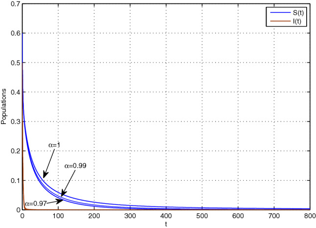
Again, we consider the parameter set: $r=0.75;a=0.5;\beta =0.5;b=0.01;\delta =0.13;\gamma =0.9;m=0.01;d=0.1;u=0.01$ as $R_0=1.48>1$. Figure 4 shows that the EE(0.707, 0.205) is asymptotically stable. Also for the different parameter set: $r=0.6;a=0.55;\beta =0.3;b=0.001;\gamma =1;m=0.154;d=0.1;\delta =0.13;u=0.01;$ with fractional order $\alpha =0.95$, Fig. 5 shows that the EE(0.508, 0.034) is asymptotically stable (green curves). But if the $\alpha$ increases to the value ${\alpha }_0=0.95$, then we will see limit cycles are formed around EE for this particular order of differentiation and hence it proves the existence of Hopf bifurcation. If the $\alpha$ further increases, then limit cycles will be bigger. Figure 5 depicts these behaviours (red and blue curves).

Fig. 4.

Dynamical behaviour around EE

Fig. 5.

Limit cycle for fractional order $\alpha$

Choose the next parameter set: $r=0.6;a=0.55;\beta =0.8;b=0.001;\gamma =1;m=0.154;d=0.1;\delta =0.13;u=0.01;$ with fractional-order $\alpha =0.99$. Figure 6 shows that the EE(0.819, 0.039) is asymptotically stable (blue curves). But if the $\beta$ decreases to the value ${\beta }_0=0.3$, then we will see limit cycles are formed around EE for this particular $\beta ={\beta }_0$ and hence it proves the existence of Hopf bifurcation. Figure 6 shows this behaviour (red curves).

Fig. 6.

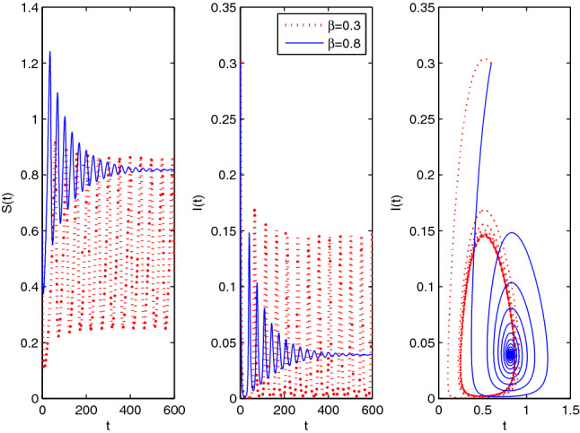
Limit cycle for level of fear $\beta$

Again, assume the parameter set: $r=0.6;a=0.55;\beta =0.4;b=0.001;\gamma =1;m=0.154;d=0.1;\delta =0.13;u=0.2;$ with fractional-order $\alpha =0.99$, Fig. 7 shows that the EE(0.703, 0.043) is asymptotically stable (blue curves). But if the u decreases to the value $u_0=0.01$, then we will see limit cycles are formed around EE for this particular $u=u_0$ and hence it confirms that the system undergoes a Hopf bifurcation. Figure 7 shows these phenomena (red curves).

Fig. 7.

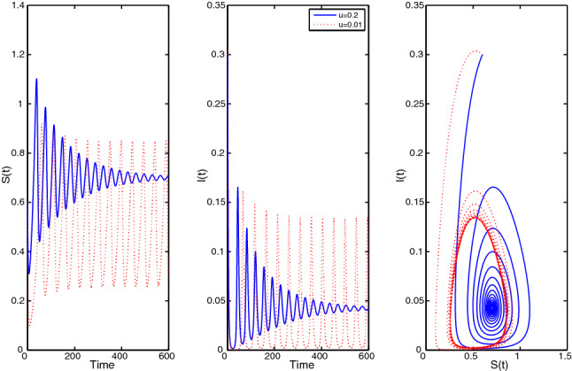
Limit cycle for disease control parameter u

Next, we choose the parameter set: $r=0.5;a=0.5;\beta =0.5;b=0.01;\gamma =0.9;m=0.01;d=0.1;\delta =0.13;u=0.01;$ with ${\alpha }_1=0.99,{\alpha }_2=0.98$, and using this, we solve system (2.3). Since for these parameters $R_0=0.986<1$ the DFE(0.17,0) is asymptotically stable. Figure 8 (left) confirms this behaviour. Finally, using the parameter set: $r=0.65;a=0.5;\beta =0.5;b=0.01;\gamma =0.9;m=0.01;d=0.1;\delta =0.13;u=0.01;$ and ${\alpha }_1=0.99,{\alpha }_2=0.98$, we solve system (2.3). Since for these parameters $R_0=1.2823>1$ the EE(0.7,0.13) is asymptotically stable. Figure 8 (right) verifies this.

Fig. 8.

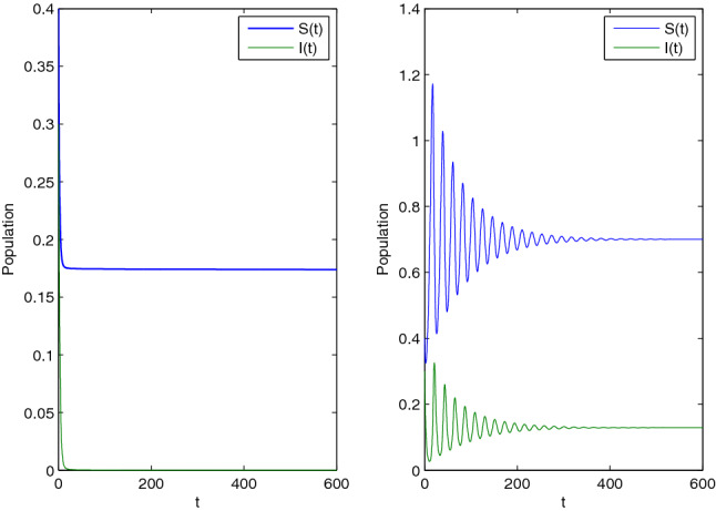
Dynamical behaviour of system (2.3) for different ${\alpha }^{\prime }s$

Discussions

In this present paper, we have proposed and analysed a new fractional-order SIS-type epidemic model with fear effect of the infectious disease and also the effect of treatment control. The fractional-order system is more naturalistic, and it brings on more affects as compared to the ordinary system or commonly known as integer-order system. The features of most of the real-world problems (or systems) assure that their model possibly more exactly formed with the fractional-order system. A higher-order system can also be modelled to a lower-order system by using fractional calculus. In case of control theory, the systems which are modelled by fractional calculus produce much better affect than the ordinary or integer-order system of differential equations.

In our proposed model systems, i.e. commensurate system (2.2) and incommensurate system (2.3), we deduced the criterion for the existence and uniqueness of various equilibrium points of the systems in several fractional-order cases. Then we examined the conditions for nonnegativity of solutions and also uniform boundedness of that solutions. Furthermore, we established sufficient conditions to check that DFE, $E^0$ and the EE, $E^{\ast }$ of system (2.2) are asymptotically stable globally by developing suitable Lyapunov functions. Further, the theoretical results are asserting by some numerical simulations. We restrict our numerical works at the EE point of proposed systems (2.2) and (2.3).

We have studied that $R_0$, the basic reproduction number of our model acts a significant purpose in local and also global stability of DFE point (Fig. 3). Also, treatment control u and the parameter of the level control $\beta$ have key role to local and also the global asymptotic stability of EE point (Fig. 4). We have demonstrated the criterion for the existence of Hopf bifurcation for commensurate system (2.2), against the parameter of the level of fear $\beta$ and also noticed that similar types of conditions can be found for the existence of Hopf bifurcation against the disease control parameter u. We have also presented the Hopf bifurcation against the parameters $\alpha ,\beta$ and u in Figs. 5, 6 and 7, respectively. In case of incommensurate system (2.3), Fig. 8 depicts the dynamical behaviour for the different fractional orders ${\alpha }_1$ and ${\alpha }_2$.

In this numerical simulation, we have applied the predictor–corrector $P{(EC)}^{m}E$ (Predict, multi-term (Evaluate, Correct), Evaluate) method Diethelm et al. (2002), Diethelm and Braunschweig (2003) and Garrappa (2010) with the help of MATLAB software. We use the implicit fractional linear multistep methods (FLMMs) as solver function for our proposed systems (2.2) and (2.3) with the fractional differential equations, and applying this method, we have described the phase portrait. Notice that $P{(EC)}^{m}E$ is modified iteration formula of the method, PECE (Predict, Evaluate, Correct, Evaluate) and Adams–Moulton algorithm.

Conclusions

We conclude that our proposed model yields efficient results and the model may serve as a tool for a wide range of utilizations in the mathematical epidemiology. In our future works, we develop and study several fractional-order epidemic models with the help of various numerical methods like Taylor series approximations method, homotopy perturbation method, Diethelma’s method, Adomian decomposition method, etc. Also in future, we stretch SIS-type epidemic model to SIR, SEIR, SEIRS model with treatment and vaccination controls in the presence of fear of the disease and apply fractional optimal control analysis of the disease control parameters which helps us to optimize the cost used in the controlling of the disease. Moreover, this mathematical model may be applied to examine the nature and also dynamics of almost every infectious disease.

Compliance with ethical standards

Conflict of Interest

On behalf of all authors, the corresponding author states that there is no conflict of interest.

References

- Clinchy M, Sheriff MJ, Zanette LY. Predator-induced stress and the ecology of fear. Funct Ecol. 2013;27(1):56–65. doi: 10.1111/1365-2435.12007. [DOI] [Google Scholar]
- Delavari H, Baleanu D, Sadati J. Stability analysis of Caputo fractional-order non linear system revisited. Non Linear Dyn. 2012;67:2433–2439. doi: 10.1007/s11071-011-0157-5. [DOI] [Google Scholar]
- Deshpande AS, Daftardar-Gejji V, Sukale YV. On Hopf bifurcation in fractional dynamical systems. Chaos Solitons Fractals. 2017;98:189–198. doi: 10.1016/j.chaos.2017.03.034. [DOI] [Google Scholar]
- Diethelm K, Braunschweig Efficient solution of multi-term fractional differential equations using P(EC)mE methods. Computing. 2003;71:305–319. doi: 10.1007/s00607-003-0033-3. [DOI] [Google Scholar]
- Diethelm K, Ford NJ, Freed AD. A predictor-corrector approach for the numerical solution of fractional differential equations. Nonlinear Dyn. 2002;29:3–22. doi: 10.1023/A:1016592219341. [DOI] [Google Scholar]
- El-Saka HAA. Backward bifurcations in fractional-order vaccination models. J Egypt Math Soc. 2015;23:49–55. doi: 10.1016/j.joems.2014.02.012. [DOI] [Google Scholar]
- El-Saka HAA, Lee S, Jang B. Dynamic analysis of fractional-order predator-prey biological economic system with Holling type II functional response. Nonlinear Dyn. 2019;96:407–416. doi: 10.1007/s11071-019-04796-y. [DOI] [Google Scholar]
- Garrappa R. On linear stability of predictor–corrector algorithms for fractional differential equations. Int J Comput Math. 2010;87:2281–2290. doi: 10.1080/00207160802624331. [DOI] [Google Scholar]
- Ghirlanda S, Frasnelli E, Vallortigara G. Intraspecific competition and coordination in the evolution of lateralization. Phil Trans R Soc. 2009;364:861–866. doi: 10.1098/rstb.2008.0227. [DOI] [PMC free article] [PubMed] [Google Scholar]
- Guo Y (2014) The Stability of Solutions for a Fractional Predator-Prey System. Abstract and Applied Analysis, Article ID 124145, 7 pages, 10.1155/2014/124145
- Hilfer R. Applications of fractional calculus in physics. River Edge: World Scientific Publishing Co., Inc; 2000. [Google Scholar]
- Jana S, Nandi SK, Kar TK. Complex dynamics of an SIR epidemic model with saturated incidence rate and treatment. Acta Biotheoretica. 2016;64:65–84. doi: 10.1007/s10441-015-9273-9. [DOI] [PubMed] [Google Scholar]
- Jana S, Haldar P, Kar TK. Optimal control and stability analysis of an epidemic model with population dispersal. Chaos Solitons Fractals. 2017;83:67–81. doi: 10.1016/j.chaos.2015.11.018. [DOI] [Google Scholar]
- Jana S, Haldar P, Kar TK. Mathematical analysis of an epidemic model with isolation and optimal controls. Int J Comput Math. 2017;94(7):1318–1336. doi: 10.1080/00207160.2016.1190009. [DOI] [Google Scholar]
- Jingjing H, Hongyong Z, Linhe Z. The effect of vaccines on backward bifurcation in a fractional-order HIV model. Nonlinear Anal Real World Appl. 2015;26:289–305. doi: 10.1016/j.nonrwa.2015.05.014. [DOI] [Google Scholar]
- Kar TK, Jana S. A theoretical study on mathematical modelling of an infectious disease with application of optimal control. BioSystems. 2013;111:37–50. doi: 10.1016/j.biosystems.2012.10.003. [DOI] [PubMed] [Google Scholar]
- Kar TK, Jana S. Application of three controls optimally in a vector-borne disease—a mathematical study. Commun Nonlinear Sci Numer Simul. 2013;18:2868–2884. doi: 10.1016/j.cnsns.2013.01.022. [DOI] [Google Scholar]
- Karthikeyan P, Arul R. Uniqueness and stability results for non-local impulsive implicit hadamard fractional differential equations. J Appl Nonlinear Dyn. 2020;9:23–29. doi: 10.5890/JAND.2020.03.002. [DOI] [Google Scholar]
- Kermack WO, Mckendric AG. Contribution to the mathematical theory of epidemics. Proc R Soc Lond Ser. 1927;115:700–721. [Google Scholar]
- Khatua A, T. K. K, Nandi SK, Jana S, Kang Y. Impact of human mobility on the transmission dynamics of infectious diseases. Energy Ecol Environ. 2020;5:389–406. doi: 10.1007/s40974-020-00164-4. [DOI] [PMC free article] [PubMed] [Google Scholar]
- Kilbas A, Srivastava H, Trujillo J. Theory and application of fractional differential equations. New York: Elsevier; 2006. [Google Scholar]
- Li Y, Chen YQ, Podlubny I. Mittag-Leffler stability of fractional-order nonlinear dynamic systems. Automatica. 2009;45:1965–1969. doi: 10.1016/j.automatica.2009.04.003. [DOI] [Google Scholar]
- Li Y, Chen Y, Podlubny I. Stability of fractional-order nonlinear dynamic systems: Lyapunov direct method and generalized Mittag–Leffler stability. Comput Math Appl. 2010;59:1810–1821. doi: 10.1016/j.camwa.2009.08.019. [DOI] [Google Scholar]
- Li H, Jing Z, Yan CH, Li J, Zhidong T. Dynamical analysis of a fractional-order predator-prey model incorporating a prey refuge. J Appl Math Comput. 2016;54:435–449. doi: 10.1007/s12190-016-1017-8. [DOI] [Google Scholar]
- Liang S, Wu R, Chen L. Laplace transform of fractional-order differential equations. Electron J Differ Equ. 2015;2015(139):1–15. [Google Scholar]
- Maji C, Kesh D, Mukherjee D. Bifurcation and global stability in an eco-epidemic model with refuge. Energy Ecol Environ. 2019;4:103–115. doi: 10.1007/s40974-019-00117-6. [DOI] [Google Scholar]
- Miller KS, Ross B. An introduction to the fractional calculus and fractional differential equations. New York: Wiley; 1993. [Google Scholar]
- Murray JD. Mathematical biology. Berlin: Springer; 2002. [Google Scholar]
- Odibat Z, Shawagfeh N. Generalized Taylors formula. Appl Math Comput. 2007;186:286–293. [Google Scholar]
- Petras I. Fractional-order nonlinear systems: modeling analysis and simulation. Beijing: Higher Education Press; 2011. [Google Scholar]
- Podlubny I. Fractional differential equations. San Diego: Academic Press; 1999. [Google Scholar]
- Sabatier J, Agrawal OP, Tenreiro Machado JA. Advances in fractional calculus: theoretical developments and applications in physics and engineering. Berlin: Springer; 2007. [Google Scholar]
- Sengupta S, Ghosh U, Sarkar S, Das S. Prediction of ventricular hypertrophy of heart using fractional calculus. J Appl Nonlinear Dyn. 2020;9:287–305. doi: 10.5890/JAND.2020.06.010. [DOI] [Google Scholar]
- Venturino E, Roy PK, Basir FA, Datta A. A model for the control of the mosaic virus disease in Jatropha curcas plantations. Energy Ecol Environ. 2016;1:360–369. doi: 10.1007/s40974-016-0033-8. [DOI] [Google Scholar]
- Wang X, Zanette L, Zou X. Modelling the fear effect in predator–prey interactions. J Math Biol. 2016;73(5):1179–1204. doi: 10.1007/s00285-016-0989-1. [DOI] [PubMed] [Google Scholar]
- Worldbank (2018) Fertility rate, total (births per woman)—Hong Kong SAR, China, https://data.worldbank.org, Accessed 6 July 2018
- Yadav VK, Shukla VK, Srivastava M, Das S. Stability analysis, control of simple chaotic system and its hybrid projective synchronization with fractional Lu system. J Appl Nonlinear Dyn. 2020;9:93–107. doi: 10.5890/JAND.2020.03.008. [DOI] [Google Scholar]
- Zhou Y, Yang K, Zhou K, Liang Y. Optimal Vaccination Policies for an SIR Model with limited resources. Acta Biotheor. 2014;62:171–181. doi: 10.1007/s10441-014-9216-x. [DOI] [PubMed] [Google Scholar]