Deep Convolutional Radiomic Features on Diffusion Tensor Images for Classification of Glioma Grades

Abstract

The grading of glioma has clinical significance in determining a treatment strategy and evaluating prognosis to investigate a novel set of radiomic features extracted from the fractional anisotropy (FA) and mean diffusivity (MD) maps of brain diffusion tensor imaging (DTI) sequences for computer-aided grading of gliomas. This retrospective study included 108 patients who had pathologically confirmed brain gliomas and DTI scanned during 2012–2018. This cohort included 43 low-grade gliomas (LGGs; all grade II) and 65 high-grade gliomas (HGGs; grade III or IV). We extracted a set of radiomic features, including traditional texture, morphological, and novel deep features derived from pre-trained convolutional neural network models, in the manually-delineated tumor regions. We employed support vector machine and these radiomic features for two classification tasks: LGGs vs HGGs, and grade III vs IV. The area under the receiver operating characteristic (ROC) curve (AUC), accuracy, sensitivity, and specificity was reported as the performance metrics using the leave-one-out cross-validation method. When combining FA+MD, AUC = 0.93, accuracy = 0.94, sensitivity = 0.98, and specificity = 0.86 in classifying LGGs from HGGs, while AUC = 0.99, accuracy = 0.98, sensitivity = 0.98, and specificity = 1.00 in classifying grade III from IV. The AUC and accuracy remain close when features were extracted from only the solid tumor or additionally including necrosis, cyst, and peritumoral edema. Still, the effects in terms of sensitivity and specificity are mixed. Deep radiomic features derived from pre-trained convolutional neural networks showed higher prediction ability than the traditional texture and shape features in both classification experiments. Radiomic features extracted on the FA and MD maps of brain DTI images are useful for noninvasively classification/grading of LGGs vs HGGs, and grade III vs IV.

Introduction

Gliomas are the most common type of primary brain tumor in adults and a critical cause of brain cancer mortality [1]. According to the World Health Organization (WHO), gliomas can be classified into four grades in terms of the pathologic evaluation of the tumor [2]. Grades I and II are low-grade gliomas (LGGs) with more favorable outcomes [1–3]. Grades III and IV are high-grade gliomas (HGGs) and they are malignant. HGGs indicate a poor prognosis [1, 3, 4]: the 5-year survival of Grade IV patients (i.e., glioblastoma) is approximately 10%, while Grade III tumors have a slightly better prognosis than glioblastoma. An accurate classification between LGGs and HGGs is critical for clinical planning of treatment strategies and predicting prognosis and treatment response. There is a need for a noninvasive approach to differentiate glioma grades both at initial diagnosis and at follow-up in the clinical management of gliomas [5].

Radiological imaging such as brain magnetic resonance imaging (MRI), is a noninvasive tool for glioma diagnosis [6, 7]. Routine brain MRI such as T2-weighted, fluid attenuation inversion recovery (FLAIR), and contrast-enhanced T1-weighted sequences can illuminate the size, shape, lesion structure, and enhancement patterns of gliomas. Due to the overlap of the imaging features between LGGs and HGGs, classification with routine MR imaging sequences is often unreliable [8]. With the development of MRI techniques, advanced procedures, such as diffusion-weighted imaging (DWI) and diffusion tensor imaging (DTI) [9, 10], have been incorporated in standard MRI examinations to assist preoperative glioma assessment. DTI is an in vivo diffusion imaging technique for assessing the directionality (anisotropy) and magnitude (diffusivity) of water diffusion, revealing the microstructural architecture of both normal and diseased tissues [10]. The conventional metrics of DTI are the mean diffusivity (MD) and fractional anisotropy (FA) [9–11]. MD describes the rotationally invariant magnitude of water diffusion within tissues. There is an inverse relationship between the cellularity and the MD value of gliomas [9]. FA expresses the orientation of the tissue microstructure. Preliminary studies showed that some characteristics of the FA appear to be useful for differentiating LGGs and HGGs [9, 10], but FA was not shown to be differential for glioma grades in some other reported studies [11, 12]. The brain DTI is still under-investigated in terms of its potential/capability for helping glioma grading.

Radiomics is an approach that quantifies the tumor phenotypes by extracting a large number of quantitative imaging features [13, 14]. This quantitative analysis method can characterize tumor properties in a non-invasive manner, and it also can be used as a powerful tool to investigate biomarkers that can assist the diagnosis and prognosis of diseases along with other clinical parameters [15, 16]. The radiomics approach follows two processes [13, 14, 17]: (a) extracting many quantitative features from medical images that represent structural, physio-pathologic, and genetic characteristics of tissues/diseases; and (b) building machine-learning models to classify these imaging features for an outcome. Promising effects have been reported in many radiomics-based cancer studies. Few studies were conducted for glioma grading by extracting features on structural MR images [18](T1- and T2-weighted images) and textural analysis on apparent diffusion coefficient (ADC) maps was identified to be effective in discriminating glioma grades [19].

While it is relatively easy to diagnose glioma grading on current MR techniques, particularly in developed countries, in many developing countries, radiologists underperform those in developed countries and thus they may still need additional help in diagnosing gliomas due to several reasons: (1) they lack experience, (2) they have not received adequate training like in large academic medical centers, and (3) they have to read a much larger volume of images in daily clinical duties that may lead to low efficiency and potential misdiagnosis. Thus, computerized methods or models may still provide a potential useful tool to augment those radiologists for glioma grading. In this study, we attempted to evaluate the effects of radiomics analyses of MD and FA maps based on segmented tumor volume in the preoperative classification of different glioma grades. We compared the results using two different sizes of tumor regions segmented manually by radiologists. Unlike previous work using only a single MRI slice [18], we utilize 3D features in radiomics analysis. Also, our radiomic features included not only common shape/morphological and texture features but also different forms of structure or texture features extracted from the shallow layers of pre-trained convolutional neural networks (CNNs) [20]. The effects of these different types of radiomic features were evaluated by feature selection and machine learning-based classification tasks.

Material and Methods

Study Cohort

The institutional review board approved this retrospective study of our institution, and informed consent from patients was waived. A total of 136 patients diagnosed from November 2012 to May 2018 were identified for this study. Inclusion criteria were: (1) Patients with pathologically confirmed newly diagnosed gliomas according to the fourth edition of the WHO classification criteria [2]; (2) patients with preoperative MRI on 3T scanners with DTI sequences acquired prior to any treatments and operations. Among them, 28 patients were excluded for the following reasons: (i) Patients with suboptimal image quality due to motion or susceptible artifacts (n = 7); (ii) lesions with hemorrhage (n = 2); (iii) irretrievable images/sequences (n = 17); (iv) WHO I lesion too small to be analyzed (n = 2). Thus, 108 patients were included in the final analysis.

MRI Protocol

All patients were examined with the same imaging acquisition protocol on a 3T whole-body MRI system (Signa HDxt, GE Medical Systems, Milwaukee, Wisconsin) with an eight-channel head coil. The MRI protocol consists of a T1 inversion recovery (IR) sequence, a T2-weighted sequence, a FLAIR sequence, and an axial T1-Contrast Enhanced (CE) sequence using the contrast agent Gadodiamide (Omniscan, GE Healthcare, Ireland) with a dose of 0.1 mmol/kg of body weight and at the rate of 2 mL/s. Before the gadolinium injection, DTI was acquired for every patient. The DTI was performed axially using a single-shot echo-planar imaging (EPI) sequence with the following parameters: TR/TE = 8000/88 ms, matrix size = 128 × 128, FOV = 240 mm × 240 mm, slice thickness = 5.0 mm, slice gap = 0 mm, diffusion gradient encoding in 30 directions, diffusion weighting factors (b value) were b = 1000 s/mm² and b = 0 s/mm² (no diffusion gradient). The DTI acquisition time was 4 min and 24 s.

After the acquisition, the DTI images were transferred to the workstation (Advantage Workstation 4.6; GE Medical Systems) to generate MD and FA maps. The diffusion tensor was diagonalized to yield the major (λ₁), intermediate (λ₂) and minor (λ₃) eigenvalues corresponding to the three eigenvectors in the diffusion tensor matrix [21]. MD and FA derive from the three eigenvalues (λ₁, λ₂, and λ₃). MD is a voxel-wise measure of the directionally averaged magnitude of diffusion (unit: square millimeters per second), calculated as follows (Eq. 1):

$$\mathrm{MD}=\frac{\left({\mathrm{\lambda }}_1+{\mathrm{\lambda }}_2+{\mathrm{\lambda }}_3\right)}{3}$$ 1

FA is used to measure the fraction of the total magnitude of diffusion, that is anisotropic and has a value of 0 for isotropic diffusion (λ₁ = λ₂ = λ₃) and 1 for completely anisotropic diffusion (λ₁ = >0, λ₂ = λ₃ = 0). FA was calculated as follows (Eq. 2):

$$\mathrm{FA}=\sqrt{\frac{3}{2}}\sqrt{\frac{{\left({\mathrm{\lambda }}_1-\mathrm{MD}\right)}^2+{\left({\mathrm{\lambda }}_2-\mathrm{MD}\right)}^2+{\left({\mathrm{\lambda }}_3-\mathrm{MD}\right)}^2}{{\mathrm{\lambda }}_1^2+{\mathrm{\lambda }}_2^2+{\mathrm{\lambda }}_3^2}}$$ 2

Methodology Pipeline

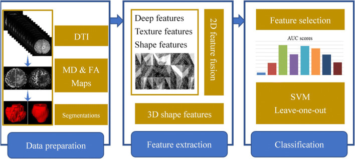
Our proposed methodology pipeline for glioma grade classification is shown in Fig. 1. In the data preparation stage, we first define and manually segment tumor regions on both the MD and FA maps. Then, a set of 329 radiomic features are extracted, followed by feature selection and support vector machine (SVM)-based machine learning classification.

Fig. 1.

The flowchart of the proposed methodology pipeline

Tumor Segmentation

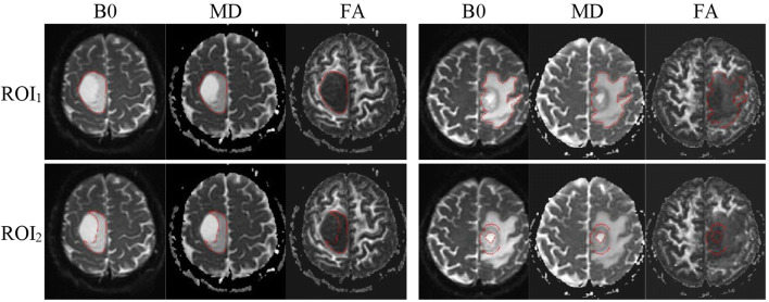
Tumor regions are first segmented manually by an experienced radiologist (with 14-year experience in the Department of Radiology) on the B0 images (DWI without diffusion sensitization) and reviewed by another senior radiologist (with 26-year maturity). The segmentation was done slice by slice using the ITK-SNAP software (version 3.6.0) (http://www.itksnap.org) and following a previously described visual inspection procedure [22]. We defined two different regions of interest (ROIs) to label the tumor regions (Fig. 2). ROI1 denotes all abnormal signals on the B0 image, including the contrast-enhancing, peritumoral edema, cyst, and necrotic regions, while ROI2 just contains the solid part of the tumor, excluding necrosis, cyst, and peritumoral edema. Tumor boundaries were identified referring to the high-signal intensity areas. The ROIs were segmented directly on the B0 image, while T1CE, T1W, and FLAIR images are allowed to access for reference for the segmentation. The segmentation masks were then transferred to the corresponding MD and FA maps for radiomic feature extraction.

Fig. 2.

Tumor region segmentation demonstration. (Left) Images of a 51-year-old male with oligodendroglioma (grade II). (Right) Images of a 64-year-old male with glioblastoma (grade IV). ROI1 denotes all abnormal signal on the B0 image, including contrast-enhancing, necrotic regions, cyst, and peritumoral edema, while ROI2 just contains the solid part of the tumor, excluding necrosis, cyst, and peritumoral edema. The ROIs were segmented on the B0 images and then transferred to the corresponding MD and FA maps

Radiomic Feature Extraction

A total of 329 candidate radiomic features were extracted from the ROIs of all MRI scans using the Image Processing toolbox provided by Matlab2016b and the third-party toolkit MatConvNet [23]. These include three different types of features, namely, convolutional deep features, texture features, and shape/morphological features (Table 1). Those features were further filtered by a feature selection step to use a much smaller set of features to build the classification models.

Table 1.

List of the 329 candidate radiomic features

Feature ID	The description of features
1–256	Novel deep convolutional features (structural/texture features)
257–272	Gray-Level Co-occurrence Matrix (GLCM) texture features
273–283	Intensity histogram and uniformity features
284–299	Wavelet texture features
300–326	Common 2D shape features, namely, eccentricity, extent, perimeter, orientation, centroid, major axis length, minor axis length, area, equivalent diameter, solidity, extrema
327–329	3D shape features, namely, volume, surface area, and spherical degree

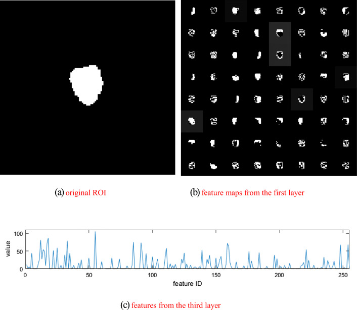
Convolutional deep features: recent studies [24] have shown that the shallow layers in deep learning CNNs convey some sufficient information of the input imaging data. Extensive experiments [25, 26] of applying pre-trained CNN models from ImageNet for different medical processing tasks had demonstrated that these pre-trained models could be used as an offline feature extractor. We followed this paradigm to extract deep convolutional radiomic features from the tumor regions. For the segmented ROI1 part, the average diameter of the tumor is 4.29 cm (range 1.67–5.80 cm), while for the segmented ROI2 region, the average diameter of the tumor is 3.69 cm (range 1.56–5.76 cm). As the size is 107 × 107 for the input of the network, we rescaled larger tumor ROIs to 107 × 107 using the nearest-neighbor interpolation algorithm. For tumor ROIs smaller than 107 × 107, we keep the original image resolution/signal by padding extra zeros to the 107 × 107 image matrix. Deep learning CNN models extract low- and high-level features at different layers. To explore the transferability of a pre-trained model VGG-f [27], we chose to use the third layer to extract imaging features from the tumor ROIs by referring to previous work [28], where the third layer represents a trade-off between performance and model depth. The corresponding structure of the network is shown in Table 2, while example feature maps extracted from the pre-trained model are shown in Fig. 3. We chose to use the VGG-f model in this study because of its relatively good generalization capability with fast speed [23] in transferring deep models to other tasks. Besides, several works of literature [24] have shown that deep learning model working in medical images do benefit from a pre-training on a large non-medical imaging dataset such as the ImageNet. A total of 256 quantitative deep radiomic features are extracted from the first 3 convolutional layers of the pre-trained model. As a robustness analysis, we also compared the overall effects of extracting radiomic features from the first four layers of the model.

Table 2.

Using the pre-trained convolutional neural network (CNN) models as a feature extractor

Structure	Convolutional neural network
Input images (107 × 107)	Conv layer 1	Conv layer 2	Conv layer 3
	64 × 11 × 11	256 × 5 × 5	256 × 3 × 3
	str. 4, pad 0, lrn, *2 pool	str. 1, pad 0, lrn, *2 pool	str. 1, pad 0

Fig. 3.

Example feature maps extracted from the pre-trained model

In the convolutional layers, the first number indicates the receptive field size as “num × size × size,” followed by the convolution stride “str.,” spatial padding “pad,” local response normalization “lrn,” and the max-pooling down-sampling factor “pool.”

Handcrafted texture features: for commonly used handcrafted texture features, and we utilized two types of features, i.e., Gray-Level Co-occurrence Matrix (GLCM) and wavelet features. Before computing the GLCM features, a preprocessing step, image filtration, is applied, where a Laplacian of Gaussian band-pass filter was applied with a step size of 3 for image denosing. When extracting GLCM features, the gray-level is set with ten. We use the features of contrast, correlation, energy, and homogeneity in GLCM from angles 0, 45, 90, and 135, respectively. Wavelet features were extracted with the coefficients of low and high frequency at level 2. In total, 43 texture features were extracted.

Shape/Morphological features: for 2D shape features, we extracted a set of 27 geometric features of the ROIs from an MRI slice, including eccentricity, extent, perimeter, orientation, centroid, major axis length, area, solidity, extrema, equiv-diameter, and minor axis length features etc. These 2D features extracted from all 2D MRI slices are combined. Besides, three volumetric 3D shape features are computed from the tumor volume, namely, volume, superficial area, and degree of sphericity.

Classification and Statistical Analysis

In this work, we adopt the SVM to build classification models. To reduce data redundancy and the number of powerful features, we adapted the iterative information gain algorithm [29] to perform feature selection under the leave-one-out cross-validation strategy and used AUC as the optimization criteria. Note that when conducting feature selection, the model is only trained with the training set instead of all the data. In each iteration, every feature is attempted to be added into the selected feature set, and the one improves the AUC score mostly is chosen in a given iteration. The selected set of features is updated from iteration to iteration, yielding the final results when none of the remaining features could further improve the AUC.

The selected features were fed into an SVM classifier with a linear kernel (we used the SVM implementation provided in Matlab 2016b) for classification. All the SVM parameters are fixed across all of the experiments. We investigated two glioma grading experiments, i.e., the classification between LGGs and HGGs as well as between WHO III and WHO IV grades. Considering our sample size, we utilized the leave-one-out cross-validation to evaluate the performance of the classification models. The goal of cross-validation is to test the model’s ability to predict new data and to give an insight into how the model will generalize to an independent dataset. Leave-one-out cross-validation reserves one sample for test and the rest samples for training. During the experiments, all the samples will be used as a test sample once, where the final results augment from all tests.

In addition, we further explored the performance of the method using the pure deep learning modeling method. In this method, we utilized the VGG model where the convolutional layers are fixed, and the fully connected layers are adapted and fine-tuned with our own image data. Five-fold cross-validation is conducted, and we trained 100 iterations as the network has converged. The performance of using deep learning modeling alone is compared to the effect of using the combination of deep learning and radiomics.

The area under the receiver operating characteristic (ROC) curve (AUC), accuracy, sensitivity, and specify was measured. All statistical analyses were performed using the IBM SPSS Statistics (v. 19.0; Chicago, IL). The level of confidence was kept at 95% and results with p < 0.05 were considered statistically significant. The chi-square test was used to assess whether the constituent ratios of sex and age are significantly different between groups. All experiments were implemented and run on a desktop computer with an Intel Core I7-7800X 3.50GHz*12 and two Titan X Graphical Processing Units (GPUs).

Results

Among the 108 patients, 43 were LGGs, and the remaining 65 were pathologically confirmed HGGs (25 WHO III and 40 WHO IV patients). The clinical characteristics of the study cohort are summarized in Table 3. Statistical results listed in Table 3 show that no significant differences were found between LGGs and HGGs for all the listed factors.

Table 3.

Baseline demographics and clinical characteristics of the 108 patients

	Low grade	High grade	P value
Patients (N/%)	39.81% (43/108)	60.19% (65/108)	NA
Ages(rang, years)	43.2(24–66)	51.3(21–78)	0.072
0–30	11.63%(5/43)	7.69%(5/65)
31–60	83.72%(36/43)	72.31%(47/65)
> 60	4.65%(2/43)	20%(13/65)
Gender (N/%)			0.77
Male	58.14% (25/43)	55.38% (36/65)
Female	41.86% (18/43)	44.62% (29/65)
Histologic subtype (N/%)	Diffuse astrocytoma	Anaplastic astrocytoma	NA
	51.16% (22/43)	16.92% (11/65)
	Oligodendroglioma	Anaplastic oligodendroglioma
	41.86% (18/43)	20.00% (13/65)
	Oligoastrocytoma	Anaplastic oligoastrocytoma
	6.98% (3/43)	1.54% (1/65)
		Glioblastoma
		61.54% (40/65)

Gliomas Grade Classification: LGGs Vs HGGs

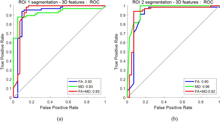
The ROCs of the selected features in different DTI maps are shown in Fig. 4. For a broader tumor region (i.e., ROI1), MD achieved a marginally higher AUC of 0.93 in comparison to the 0.92 yielded by FA. Likewise, for a smaller tumor region (ROI2), the AUC of FA is 0.90, and improvement is observed for MD with an AUC of 0.96. In both scenarios, MD outperforms FA. When combining the features selected separately from FA and MD together, AUC is 0.93 for ROI1 and 0.92 for ROI2, respectively; there is no noticeable improvement when fusing FA and MD compared to using the FA or MD alone. Also, when we used the first four layers for feature extraction, the AUC is 0.93 for ROI1 and 0.92 for ROI2 on the combination of MD and FA (ROC curves not plotted in Fig. 4).

Fig. 4.

ROCs for distinguishing LGGs vs HGGs: a using features extracted from ROI1; b using features extracted from ROI2

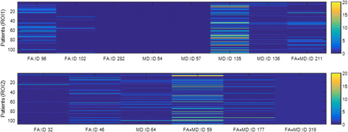
The IDs of the selected features are listed in Table 4. Referring to Table 1, all selected features here are from the deep convolutional features, except feature #282 (wavelet texture features) and #319 (one of extrema points in the region). We also find that the number of features is not correlated with the classification performance. For example, it is a single feature that leads to the highest AUC for ROI1 on FA+MD (i.e., feature #211; AUC = 0.93) and ROI2 on MD (i.e., feature #64; AUC = 0.96). Figure 5 shows the weight distribution of the 211th and 64th features, where we can see that the distribution of these two most predictive features spans a range of 0 to 10.

Table 4.

The IDs of the selected features in classifying LGGs from HGGs and WHO III from WHO IV. Refer to Table 1 for the ID definition

	ROI1 features’ IDs	ROI2 features’ IDs
LGGs vs HGGs
FA	96,102,282	32 46
MD	54 57 135 136	64
FA+MD (average)	211	59 177 319
WHO III vs WHO IV
FA	220,253	215,317
MD	157	106,131,165
FA+MD (average)	58 67 99,317	51,189

Fig. 5.

Weight distributions of the selected features in classifying LGGs from HGGs

As shown in Table 5, the accuracy, sensitivity, and specificity, the combination of the FA and MD, brings increased performance for some but not for all scenarios. The effects of comparing the two ROIs are also mixed.

Table 5.

The classification performance in terms of accuracy, sensitivity, and specificity for classifying LGGs from HGGs and WHO III from WHO IV

	Accuracy		Sensitivity		Specificity
	ROI1	ROI2	ROI1	ROI2	ROI1	ROI2
LGGs vs HGGs.
FA	0.93	0.91	0.95	0.97	0.88	0.81
MD	0.91	0.94	0.88	1.00	0.95	0.86
FA+MD	0.94	0.94	0.98	0.94	0.86	0.93
WHO III vs WHO IV
FA	0.94	0.83	0.98	0.95	0.88	0.64
MD	0.89	0.83	0.88	0.98	0.92	0.60
FA+MD	0.98	0.97	0.98	0.98	1.00	0.96

Gliomas Grade Classification: WHO III Vs WHO IV

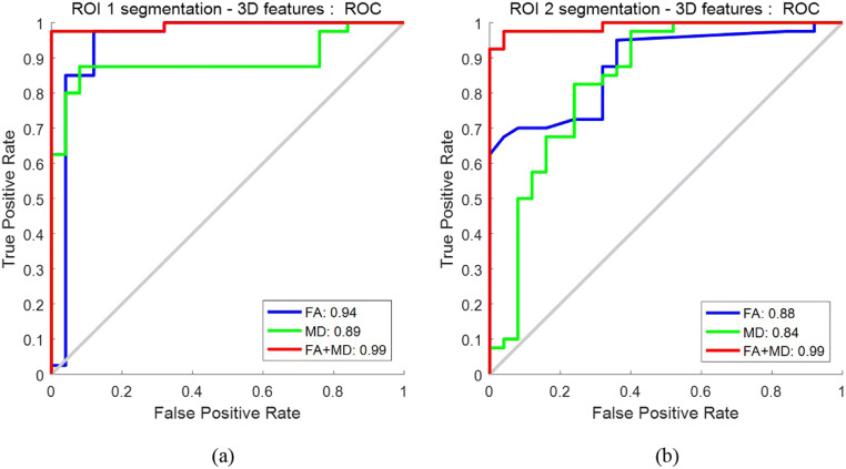
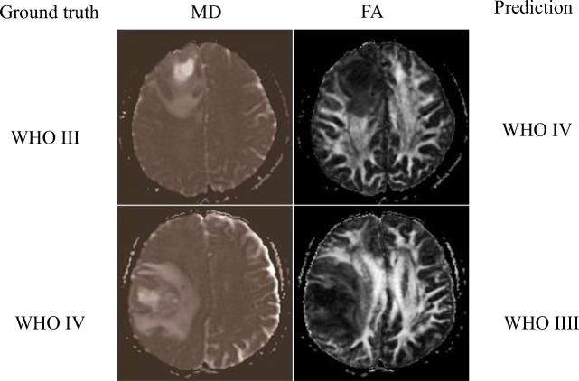
Like “Gliomas Grade Classification: LGGs Vs HGGs”, experiments on classifying WHO III vs IV grade were conducted, and similar results were reported here. As shown in Fig. 6, on both ROI1 and ROI2, FA outperforms MD, and when the two modalities were combined, a substantial increase of AUC was observed, and the AUC goes high up to 0.99 on both ROIs. The patterns of the effects are different from those in classifying LGGs from HGGs (“Gliomas Grade Classification: LGGs Vs HGGs”). Also, when we used the first four layers for feature extraction, the AUC is 0.96 for ROI1 and 0.97 for ROI2 on the combination of MD and FA (ROC curves not plotted in Fig. 6). Figure 7 shows a false positive example and a false negative example. According to the MD maps of the tumors, there are obvious edema, necrosis, and cystic degeneration, so it is difficult to grade them between WHO III and IV. The prediction model has mistakenly classified them.

Fig. 6.

ROCs for distinguishing WHO III vs IV grade: a using features extracted from ROI1; b using features extracted from ROI2

Fig. 7.

Examples of false-positive and false-negative between WHO III and IV grade

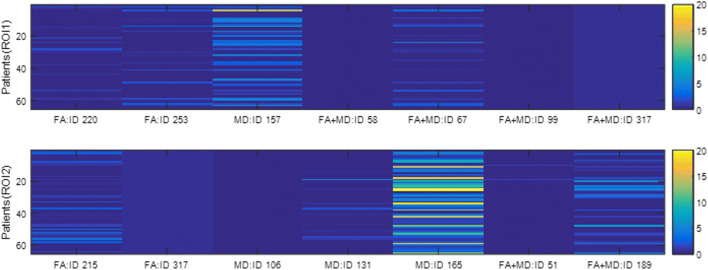
Similarly, Table 4 shows that most selected features are still from deep convolutional features except the 317th feature (one of extrema points in the region). Figure 8 indicates that the 317th feature has a quite small variation while it is helpful for the classification task.

Fig. 8.

Weight distributions of the selected features in classifying WHO III vs IV grade

In Table 5, we can see that ROI1 generally has better performance than ROI2. Note that the specificity on ROI2 is substantially low (i.e., 0.64 and 0.60) for either the FA or MD map. However, when combining the two maps, the specificity is significantly boosted up to an AUC of 0.96.

The classification results of using deep learning modeling alone are shown in Table 6. As can be seen, the combination of deep learning and radiomics outperforms the deep learning modeling alone.

Table 6.

The classification AUCs using deep learning alone for classifying LGGs from HGGs and WHO III from WHO IV

	ROI1 AUC	ROI2 AUC
LGGs vs HGGs
FA+MD	0.75	0.68
WHO III vs WHO IV
FA+MD	0.85	0.81

Discussion

Accurate grading of brain gliomas is essential for clinical therapeutic planning. In this study, we employed a radiomics approach to perform automated classification for brain gliomas using the DTI sequences in brain MRI. We focused on the FA and MD two different modalities generated from the DTI sequences. We assembled a set of radiomic features including deep features extracted from offline pre-trained deep learning models and typical texture and morphological features. In the two classification scenarios, we showed that FA, MD, or their combination, can achieve a promising performance to distinguish LGGs from HGGs, and WHO III vs IV grade.

A new aspect of our study is the use of the DTI sequences. Unlike the routine T1, T2, FLAIR, or T1-CE sequences, DTI is usually not a standard MRI sequence but often included for preoperative assessment at our institution. Preliminary evidence supports the potential of DTI data as an imaging biomarker for integrated glioma diagnosis [10, 12, 30–32]. MD and FA derived from DTI are commonly used parameters in related imaging study literature as well. MD and FA can provide complementary structure information to improve tumor characterization. MD correlates with the cellularity of tumor tissues through altered diffusion values due to increased cellular density of glioma tissues. FA represents the directionality of the diffusion process and reflects the cellular organization of tumors as well as their microenvironment, the extracellular matrix. In the literature, FA values have been shown to indicate malignancy of gliomas and are associated with cell density and proliferation in human glioblastoma as well as WHO grades [30, 31]. All these shreds of evidence may help partly interpret why the quantitative radiomic features derived from FA and MD are capable of classification of the glioma grades.

It is worth to point out the importance of multi-parametric MR imaging features in brain tumor diagnosis and grading. Tian [17] et al. showed that diffusion-weighted imaging features (ADC, distributed diffusion coefficients, intravoxel incoherent motion) had a comparable effect to the structural imaging features (T1, T2, CE-T1 sequences), while the combination of them achieved the highest performance compared to either of them alone. Cho [33] et al. used open-source data from the MICCAI Brain Tumor Segmentation 2017 Challenge (BraTS 2017). They achieved an average accuracy of 0.9292 and AUC of 0.9400 using three classifiers with fivefold cross-validation. Similar findings were found in another study [34] where the most predictive texture features were the CE-T1-derived entropy and ADC-based homogeneity. Furthermore, in classifying and grading pediatric posterior fossa tumors (medulloblastomas, pilocytic astrocytomas, and ependymomas) [35], the histogram and texture features extracted from ADC images were more predictive than the CE-T1WI and T2WI images. According to a prognosis prediction study on HGGs [36], ADC-derived texture features have a similar predictive effect on age, tumor stage, and surgical procedures. The value of ADC texture features was also shown in other studies such as differentiating glioblastomas and other tumors [37]. In general, while typical structural imaging sequences (T1 and T2) may be more vulnerable to some of the image scanning parameters and reconstruction algorithms [38], the diffusion-based imaging sequences reveal important capability in characterizing and grading the brain tumors. The effects of these different imaging sequences and their combination concerning specific tumor characterization tasks merit further investigation in future work. Unfortunately, as many cases in our study cohort had their structural MRI scanning outside of our institution, those imaging sequences are not fully available to us to do a comparative experiment. Therefore, we mainly focused on the DTI sequences in this work.

A unique aspect of this study is that we included the deep convolutional features extracted from pre-trained deep learning models in our feature set. Usually, radiomics studies just include conventional texture and shape/morphological features. In the principal analysis, we extracted deep learning features from the first three layers of the model. Our experiments show that the deep features are overall more predictive of glioma grades than the conventional texture and morphological features. We also compared the effects of using the first four layers and found they are overall comparable to the first three layers. Currently, it is not straightforward to directly interpret these deep features, since they are generated indirectly from complicated convolutional network processes. At the concept level, this kind of deep feature can be considered as a type of structural or “texture” feature, possibly characterizing the tumor heterogeneity information. There are several studies reported in the literature showing that this kind of offline deep radiomic feature can do an excellent job in outcome prediction. In principle, shallower layers of convolutional networks generate more general and a higher number of features, while the deeper layers carry more semantic but less generalizable information and a relatively smaller set of features for classification. This kind of choice on how many layers to use for feature extraction often rely on experience, actual model performance, computational cost, and the nature of tasks. While conventional radiomic features (such as textures) have been well recognized in their predictive ability, the observations on the performance of the features extracted from deep learning models are exciting and worth further investigation in future work.

There are several related studies on this topic in the literature. Because of the differences in exact study purpose, dataset, sample size, patient population/race, and the specific modeling method, a direct comparison of performance across these studies needs to be made with caution. Here we put the related results in context for reference. To accurately classify genetic mutations in gliomas, Chang [39] et al. used their own data to train a CNN as a feature extractor, which was similar to ours, and their classification accuracy values are 94% for IDH1 mutation status, 92% for 1p/19q codeletion, and 83% or MGMT promotor methylation status. Korfiatis [40] et al. directly explored the ability of predicting MGMT methylation status without the need for a distinct tumor segmentation step. They found that the ResNet50 (50 layers) architecture was the best performing model, achieving an accuracy of 94.90% for the test set. Zhou [41] et al. combined the conventional imaging features with patient’s age to predict Isocitrate dehydrogenase (IDH) and1p/19q codeletion status, showing a promising accuracy.

We also tested and compared the effects of two different sizes of the brain tumor regions in terms of ROI1 and ROI2. In both the two classification tasks, the results of the two ROIs are close to each other when we use the combination of FA and MD maps. However, when we make the comparisons individually for FA or MD, the effects are mixed. In classifying LGGs from HGGs, ROI2 is slightly better or comparable to ROI1, indicating that the solid tumor region (ROI2) itself may be already capable of such grading between LGGs and HGGs. In contrast, in classifying WHO III vs IV grade, ROI2 performs lower than ROI1 when using FA or MD alone, indicating that for a relatively more difficult grade classification task, the region of only solid tumor may not be adequate; interestingly, the effect becomes close between ROI1 and ROI2 when we use the combined data of the FA and MD. This may indicate that additional information from the two-modality fusion may be gained to complement the information carried in the non-solid tumor regions (i.e., necrosis, cyst, and peritumoral edema). This hypothesis, of course, will need further studies to look into more profound on the relationship of tumor regions and modalities for grade classification.

Our study has some limitations. First, the patient population was relatively small and from a single institution. Although we have used cross-validation to try to mitigate potential over-fitting, our study is still at the risk of over-fitting, as we do not have external data for an independent test. In future work, we plan to assemble a larger multi-center dataset to further evaluate our findings. We welcome researchers from the readers who have such data and interest to collaborate for follow-up studies on this topic. Second, the ROIs were manually delineated slice by slice, which can also be very time consuming and is susceptible to reader variability. Ideally, fully-automated and accurate segmentation by computerized methods is expected; we tested a couple of existing automated methods on our dataset but the segmentation effects were not satisfactory thus not used. Third, while we found that the deep features play a dominant role in the classification tasks we performed, it is not straightforward to interpret the physical meanings of these features, which may create obstacles in gaining clinical trust for using such kind of radiomic features in computerized decision-making models. Besides, we plan to test and compare the effects of some other deep learning models in a future study. Finally, we expected to make a comparison between the conventional MRI sequences and the DTI sequences for the grade classification; we feel that this study provided essential basics and experimental data to support our next-step research.

We would also like to point out that the molecular alterations that have been shown predictive of prognosis values in recent years [2, 5], such as IDH mutation, 1p/19q codeletion, were not involved in this preliminary study. At our institution, the stratification of glioma patients is still mainly based on grading. So this work serves as a foundation to enable us to continue to investigate radiomic features for molecular level analyses, such as distinguishing mutation statuses, in future work.

Conclusions

In summary, we performed a quantitative radiomics study to show that a set of brain DTI-derived imaging features can help distinguish the different grades of brain gliomas. After further evaluation, this kind of method and models may contribute to developing a clinical-decision toolkit to assist physicians in glioma grading.

Funding Information

This work was partially supported by the National Key Research and Development Plan of China (NO. 2016YFC0103100) and the National Natural Science Foundation of China (No. 61701506).

Ethics Approval and Consent to Participate

The Institutional Review Board approved this retrospective study of our institution, and the requirement for informed consent was waived.

Conflict of Interests

The authors declare that they have no conflict of interest.

References

- 1.Ostrom QT, Gittleman H, Liao P, Rouse C, Chen Y, Dowling J, Wolinsky Y, Kruchko C, Barnholtz-Sloan J. CBTRUS statistical report: primary brain and central nervous system tumors diagnosed in the United States in 2007–2011. Neuro Oncol. 2014;16(Suppl 4):iv1–i63. doi: 10.1093/neuonc/nou223. [DOI] [PMC free article] [PubMed] [Google Scholar]
- 2.Louis DN, Perry A, Reifenberger G, von Deimling A, Figarella-Branger D, Cavenee WK, Ohgaki H, Wiestler OD, Kleihues P, Ellison DW. The 2016 World Health Organization classification of tumors of the central nervous system: a summary. Acta Neuropathol. 2016;131:803–820. doi: 10.1007/s00401-016-1545-1. [DOI] [PubMed] [Google Scholar]
- 3.Weller M, van den Bent M, Tonn JC, Stupp R, Preusser M, Cohen-Jonathan-Moyal E, Henriksson R, Rhun EL, Balana C, Chinot O, Bendszus M, Reijneveld JC, Dhermain F, French P, Marosi C, Watts C, Oberg I, Pilkington G, Baumert BG, Taphoorn MJB, Hegi M, Westphal M, Reifenberger G, Soffietti R, Wick W, European Association for Neuro-Oncology (EANO) Task Force on Gliomas European Association for Neuro-Oncology (EANO) guideline on the diagnosis and treatment of adult astrocytic and oligodendroglial gliomas. Lancet Oncol. 2017;18:e315–315e329. doi: 10.1016/S1470-2045(17)30194-8. [DOI] [PubMed] [Google Scholar]
- 4.Omuro A, DeAngelis LM. Glioblastoma and other malignant gliomas: a clinical review. JAMA. 2013;310:1842–1850. doi: 10.1001/jama.2013.280319. [DOI] [PubMed] [Google Scholar]
- 5.Johnson DR, Guerin JB, Giannini C, Morris JM, Eckel LJ, Kaufmann TJ. 2016 updates to the WHO brain tumor classification system: what the radiologist needs to know. Radiographics. 2017;37:2164–2180. doi: 10.1148/rg.2017170037. [DOI] [PubMed] [Google Scholar]
- 6.Bai Y, Lin Y, Tian J, Shi D, Cheng J, Haacke EM, Hong X, Ma B, Zhou J, Wang M. Grading of gliomas by using monoexponential, biexponential, and stretched exponential diffusion-weighted MR imaging and diffusion kurtosis MR imaging. Radiology. 2016;278:496–504. doi: 10.1148/radiol.2015142173. [DOI] [PMC free article] [PubMed] [Google Scholar]
- 7.Smits M, van den Bent MJ. Imaging correlates of adult glioma genotypes. Radiology. 2017;284:316–331. doi: 10.1148/radiol.2017151930. [DOI] [PubMed] [Google Scholar]
- 8.Caulo M, Panara V, Tortora D, Mattei PA, Briganti C, Pravatà E, Salice S, Cotroneo AR, Tartaro A. Data-driven grading of brain gliomas: a multiparametric MR imaging study. Radiology. 2014;272:494–503. doi: 10.1148/radiol.14132040. [DOI] [PubMed] [Google Scholar]
- 9.Liu X, Tian W, Kolar B, Yeaney GA, Qiu X, Johnson MD, Ekholm S. MR diffusion tensor and perfusion-weighted imaging in preoperative grading of supratentorial nonenhancing gliomas. Neuro Oncol. 2011;13:447–455. doi: 10.1093/neuonc/noq197. [DOI] [PMC free article] [PubMed] [Google Scholar]
- 10.White ML, Zhang Y, Yu F, Jaffar Kazmi SA. Diffusion tensor MR imaging of cerebral gliomas: evaluating fractional anisotropy characteristics. AJNR Am J Neuroradiol. 2011;32:374–381. doi: 10.3174/ajnr.A2267. [DOI] [PMC free article] [PubMed] [Google Scholar]
- 11.Wang Q, Zhang J, Xu X, Chen X, Xu B. Diagnostic performance of apparent diffusion coefficient parameters for glioma grading. J Neurooncol. 2018;139:61–68. doi: 10.1007/s11060-018-2841-5. [DOI] [PubMed] [Google Scholar]
- 12.Jakab A, Molnár P, Emri M, Berényi E. Glioma grade assessment by using histogram analysis of diffusion tensor imaging-derived maps. Neuroradiology. 2011;53:483–491. doi: 10.1007/s00234-010-0769-3. [DOI] [PubMed] [Google Scholar]
- 13.Lambin P, Rios-Velazquez E, Leijenaar R, Carvalho S, van Stiphout R, Granton P, Zegers CM, Gillies R, Boellard R, Dekker A, Aerts HJ. Radiomics: extracting more information from medical images using advanced feature analysis. Eur J Cancer. 2012;48:441–446. doi: 10.1016/j.ejca.2011.11.036. [DOI] [PMC free article] [PubMed] [Google Scholar]
- 14.Gillies RJ, Kinahan PE, Hricak H. Radiomics: images are more than pictures, they are data. Radiology. 2016;278:563–577. doi: 10.1148/radiol.2015151169. [DOI] [PMC free article] [PubMed] [Google Scholar]
- 15.Lambin P, Leijenaar RTH, Deist TM, Peerlings J, de Jong EEC, van Timmeren J, Sanduleanu S, Larue RTHM, Even AJG, Jochems A, van Wijk Y, Woodruff H, van Soest J, Lustberg T, Roelofs E, van Elmpt W, Dekker A, Mottaghy FM, Wildberger JE, Walsh S. Radiomics: the bridge between medical imaging and personalized medicine. Nat Rev Clin Oncol. 2017;14:749–762. doi: 10.1038/nrclinonc.2017.141. [DOI] [PubMed] [Google Scholar]
- 16.Aerts HJ, et al. Decoding tumour phenotype by noninvasive imaging using a quantitative radiomics approach. Nat Commun. 2014;5:4006. doi: 10.1038/ncomms5006. [DOI] [PMC free article] [PubMed] [Google Scholar]
- 17.Tian Q et al.: Radiomics strategy for glioma grading using texture features from multiparametric MRI. J Magn Reson Imaging, 2018. 10.1002/jmri.26010 [DOI] [PubMed]
- 18.Skogen K, Schulz A, Dormagen JB, Ganeshan B, Helseth E, Server A. Diagnostic performance of texture analysis on MRI in grading cerebral gliomas. Eur J Radiol. 2016;85:824–829. doi: 10.1016/j.ejrad.2016.01.013. [DOI] [PubMed] [Google Scholar]
- 19.Ryu YJ, Choi SH, Park SJ, Yun TJ, Kim JH, Sohn CH. Glioma: application of whole-tumor texture analysis of diffusion-weighted imaging for the evaluation of tumor heterogeneity. PLoS One. 2014;9:e108335. doi: 10.1371/journal.pone.0108335. [DOI] [PMC free article] [PubMed] [Google Scholar]
- 20.Tajbakhsh N, Shin JY, Gurudu SR, Hurst RT, Kendall CB, Gotway MB, Liang J. Convolutional neural networks for medical image analysis: full training or fine tuning. IEEE Trans Med Imaging. 2016;35:1299–1312. doi: 10.1109/TMI.2016.2535302. [DOI] [PubMed] [Google Scholar]
- 21.Mori S, Zhang J. Principles of diffusion tensor imaging and its applications to basic neuroscience research. Neuron. 2006;51:527–539. doi: 10.1016/j.neuron.2006.08.012. [DOI] [PubMed] [Google Scholar]
- 22.Zacharaki EI, Wang S, Chawla S, Soo Yoo D, Wolf R, Melhem ER, Davatzikos C. Classification of brain tumor type and grade using MRI texture and shape in a machine learning scheme. Magn Reson Med. 2009;62:1609–1618. doi: 10.1002/mrm.22147. [DOI] [PMC free article] [PubMed] [Google Scholar]
- 23.Vedaldi A, Lenc K. MatConvNet: convolutional neural networks for MATLAB. Proceedings of the 23rd ACM International Conference on Multimedia. 2807412:ACM. 689–692. 10.1145/2733373.2807412.
- 24.Litjens G, Kooi T, Bejnordi BE, Setio A, Ciompi F, Ghafoorian M, van der Laak J, van Ginneken B, Sánchez CI. A survey on deep learning in medical image analysis. Med Image Anal. 2017;42:60–88. doi: 10.1016/j.media.2017.07.005. [DOI] [PubMed] [Google Scholar]
- 25.Oktay O, Bai W, Lee M, Guerrero R, Kamnitsas K, Caballero J, de Marvao A, Cook S, O 'regan D, Rueckert D. Multi-input Cardiac Image Super-resolution using Convolutional Neural Networks. 2016. 246–254. 10.1007/978-3-319-46726-9_29
- 26.Antropova N, Huynh B, Giger M. SU-D-207B-06: predicting breast cancer malignancy on DCE-MRI data using pre-trained convolutional neural networks. Med Phys. 2016;43:3349–3350. doi: 10.1007/978-3-319-46726-9_29. [DOI] [Google Scholar]
- 27.Chatfield K, Simonyan K, Vedaldi A, Zisserman A. Return of the devil in the details: delving deep into convolutional nets. 2014. [Google Scholar]
- 28.Paul R, Hawkins SH, Schabath MB, Gillies RJ, Hall LO, Goldgof DB. Predicting malignant nodules by fusing deep features with classical radiomics features. J Med Imaging (Bellingham) 2018;5:011021. doi: 10.1117/1.JMI.5.1.011021. [DOI] [PMC free article] [PubMed] [Google Scholar]
- 29.Franklin J. The elements of statistical learning: data mining, inference and prediction. Publ Am Stat Assoc. 2010;99:567–567. doi: 10.1007/BF02985802. [DOI] [Google Scholar]
- 30.Jiang L, Xiao CY, Xu Q, Sun J, Chen H, Chen YC, Yin X. Analysis of DTI-derived tensor metrics in differential diagnosis between low-grade and high-grade gliomas. Front Aging Neurosci. 2017;9:271. doi: 10.3389/fnagi.2017.00271. [DOI] [PMC free article] [PubMed] [Google Scholar]
- 31.Server A, Graff BA, Josefsen R, Orheim TE, Schellhorn T, Nordhøy W, Nakstad PH. Analysis of diffusion tensor imaging metrics for gliomas grading at 3 T. Eur J Radiol. 2014;83:e156–e165. doi: 10.1016/j.ejrad.2013.12.023. [DOI] [PubMed] [Google Scholar]
- 32.Raja R, Sinha N, Saini J, Mahadevan A, Rao KN, Swaminathan A. Assessment of tissue heterogeneity using diffusion tensor and diffusion kurtosis imaging for grading gliomas. Neuroradiology. 2016;58:1217–1231. doi: 10.1007/s00234-016-1758-y. [DOI] [PubMed] [Google Scholar]
- 33.Cho HH, Lee SH, Kim J, Park H. Classification of the glioma grading using radiomics analysis. PeerJ. 2018;6:e5982. doi: 10.7717/peerj.5982. [DOI] [PMC free article] [PubMed] [Google Scholar]
- 34.Qin JB, Liu Z, Zhang H, Shen C, Wang XC, Tan Y, Wang S, Wu XF, Tian J. Grading of gliomas by using radiomic features on multiple magnetic resonance imaging (MRI) sequences. Med Sci Monit. 2017;23:2168–2178. doi: 10.12659/MSM.901270. [DOI] [PMC free article] [PubMed] [Google Scholar]
- 35.Rodriguez Gutierrez D, Awwad A, Meijer L, Manita M, Jaspan T, Dineen RA, Grundy RG, Auer DP. Metrics and textural features of MRI diffusion to improve classification of pediatric posterior fossa tumors. AJNR Am J Neuroradiol. 2014;35:1009–1015. doi: 10.3174/ajnr.A3784. [DOI] [PMC free article] [PubMed] [Google Scholar]
- 36.Brynolfsson P, Nilsson D, Henriksson R, Hauksson J, Karlsson M, Garpebring A, Birgander R, Trygg J, Nyholm T, Asklund T. ADC texture--an imaging biomarker for high-grade glioma. Med Phys. 2014;41:101903. doi: 10.1118/1.4894812. [DOI] [PubMed] [Google Scholar]
- 37.Kang D, Park JE, Kim YH, Kim JH, Oh JY, Kim J, Kim Y, Kim ST, Kim HS: Diffusion radiomics as a diagnostic model for atypical manifestation of primary central nervous system lymphoma: development and multicenter external validation. Neuro Oncol, 2018. 10.1093/neuonc/noy021 [DOI] [PMC free article] [PubMed]
- 38.Yang F, Dogan N, Stoyanova R, Ford JC. Evaluation of radiomic texture feature error due to MRI acquisition and reconstruction: a simulation study utilizing ground truth. Phys Med. 2018;50:26–36. doi: 10.1016/j.ejmp.2018.05.017. [DOI] [PubMed] [Google Scholar]
- 39.Chang P, Grinband J, Weinberg BD, Bardis M, Khy M, Cadena G, Su MY, Cha S, Filippi CG, Bota D, Baldi P, Poisson LM, Jain R, Chow D. Deep-learning convolutional neural networks accurately classify genetic mutations in gliomas. AJNR Am J Neuroradiol. 2018;39:1201–1207. doi: 10.3174/ajnr.A5667. [DOI] [PMC free article] [PubMed] [Google Scholar]
- 40.Korfiatis P, Kline TL, Lachance DH, Parney IF, Buckner JC, Erickson BJ. Residual deep convolutional neural network predicts MGMT methylation status. J Digit Imaging. 2017;30:622–628. doi: 10.1007/s10278-017-0009-z. [DOI] [PMC free article] [PubMed] [Google Scholar]
- 41.Zhou H, Chang K, Bai HX, Xiao B, Su C, Bi WL, Zhang PJ, Senders JT, Vallières M, Kavouridis VK, Boaro A, Arnaout O, Yang L, Huang RY. Machine learning reveals multimodal MRI patterns predictive of isocitrate dehydrogenase and 1p/19q status in diffuse low- and high-grade gliomas. J Neurooncol. 2019;142:299–307. doi: 10.1007/s11060-019-03096-0. [DOI] [PMC free article] [PubMed] [Google Scholar]