Abstract
Histology subtype prediction is a major task for grading non-small cell lung cancer (NSCLC) tumors. Invasive methods such as biopsy often lack in tumor sample, and as a result radiologists or oncologists find it difficult to detect proper histology of NSCLC tumors. The non-invasive methods such as machine learning may play a useful role to predict NSCLC histology by using medical image biomarkers. Few attempts have so far been made to predict NSCLC histology by considering all the major subtypes. The present study aimed to develop a more accurate deep learning model by clubbing convolutional and bidirectional recurrent neural networks. The NSCLC Radiogenomics dataset having 211 subjects was used in the study. Ten best models found during experimentation were averaged to form an ensemble. The model ensemble was executed with 10-fold repeated stratified cross-validation, and the results got were tested with metrics like accuracy, recall, precision, F1-score, Cohen’s kappa, and ROC-AUC score. The accuracy of the ensemble model showed considerable improvement over the best model found with the single model. The proposed model may help significantly in the automated prognosis of NSCLC and other types of cancers.
Keywords: Lung cancer, Histology, Bidirectional, Recurrent, Neural network
Introduction
Non-small cell lung cancer (NSCLC) accounts for nearly 85% of all lung cancers and a leading cause of cancer-related death worldwide [19]. Prediction of histological subtypes is an important determinant of therapy in NSCLC as it may boost the histopathological grading workup to a significant extent [2]. Major NSCLC subtypes are lung adenocarcinoma and squamous cell carcinoma. Pathological diagnosis of NSCLC often experiences difficulties, as most NSCLC is detected at an advanced stage and samples got from surgical resection are tiny with limited tumor content [1]. This affects the biopsy results, and a proper histology subtype prediction may not be very easy for the radiologists or oncologists. With the advances in precision medicine, medical image biomarkers provide an immense improvement in characterizing a heterogeneous tumor, compared with genomic biomarkers [18]. Thus, there is a need for further study of histological prediction in NSCLC [5] by using non-invasive procedures.
Related Work
Many studies have so far been conducted to classify NSCLC tumors either as benign or malignant [16], but only a few attempts were aimed to predict NSCLC histology subtypes by using non-invasive methods [10]. Most of these studies were gene expression based [3, 7, 11], and others were traditional and advanced machine learning based [8, 9] powered by extracted image features. The gene expression–based methods could not classify non-specified NSCLC tumors successfully [4], and they sometimes lacked sensitivity [6]. Only a handful of notable works have been carried out in NSCLC histology prediction via machine learning methods. In 2016, Weimiao et al. [13] used different classification techniques to classify NSCLC histology. The study used 350 patients’ pretreatment CT images along with 440 radiomic features extracted from the segmented tumor volume. ReliefF and its variants showed improved results as far as the feature selection methods were concerned. Naive Baye’s classifier achieved the highest AUC (0.72). The prediction accuracy achieved in the study was not much high, and the study only considered adenocarcinoma and squamous cell carcinoma. Other NSCLC subtypes were not considered in the study. In 2018, Chaunzwa et al. [12] used deep learning to predict NSCLC histology. In the study, deep features were extracted from computed tomography (CT) images by using a pre-trained VGG-16 convolutional neural network. Besides CNN, the other machine learning models used in the study were as follows: K-nearest neighbors (KNN), random forest classifier (RF), and least absolute shrinkage and selection operator (LASSO). The principal component analysis was used to select features. The fully connected CNN had a pivotal performance with AUC = 0.751. The major lack in the study was that all the 157 patients had stage I NSCLC—no advanced stage NSCLC was considered. The study was aimed to identify between adenocarcinoma vs squamous cell carcinoma. This had made it a binary classification problem. In the same year, another study was conducted by Bo He et al. [14]. The aim of the study was to predict the survival status of NSCLC patients from histology. In total, 186 patients’ CT images were segmented and 1218 features were extracted through Pyradiomics. SMOTE was the data re-sampling method used in the study. Different random forest models were trained by a hyper-parameters grid search with 10-fold cross-validation, and the model had a prediction accuracy of 89.33% (AUC = 0.9296). Coudray et al. [15] also did a NSCLC histopathology classification in 2018 by using deep learning. Although the AUC was high (around 0.97), it had also considered only adenocarcinoma and squamous cell carcinoma. Thus, there is a huge scope to conduct further studies in this domain to facilitate the identification of the underlying relationship between genomic and medical image features.
Objective
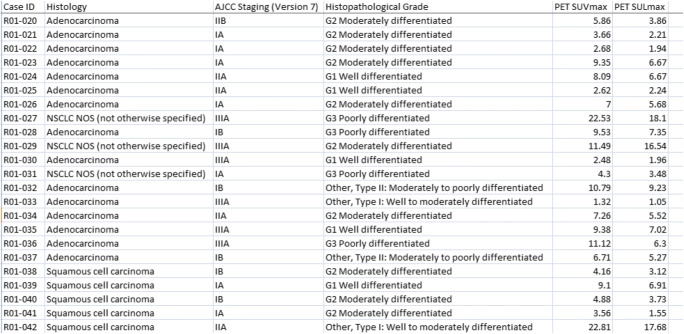
The aim of the present study is to use a deep cross-validated model averaging ensemble in the automatic prediction of NSCLC histology. Unlike its predecessors, the study includes a third NSCLC histology subtype named not otherwise specified (NOS) NSCLC alongside adenocarcinoma and squamous cell carcinoma. This has made the study a multiclass problem. The dataset used in the study [17] contains a cohort of 211 subjects having a diverse mix of AJCC (American Joint Committee on Cancer) staging [34] and histopathological grade (Fig. 1). This also takes the present study ahead of its earlier attempts. The model proposed in the study is a hybrid of convolutional and bidirectional recurrent neural network. The overall goal is to predict NSCLC histology in a more accurate way than its contemporary counterparts. This will help the radiologists and oncologists to detect NSCLC in a more affirmative manner and will also ease the way to plan the relevant treatment strategy. The rest of the paper is divided into the following segments: background, methodology, experiment, result, discussion, and future work.
Fig. 1.
Glimpse of the clinical dataset used in the study
Background
Recurrent neural network (RNN) and convolutional neural network (CNN) have been used in various fields [20, 21] including computer vision [22, 29]. The semi-automated prognosis of NSCLC is also on the list [23]. But a fully automated diagnosis of NSCLC histology has hardly been tried ever with these deep network techniques. Recurrent networks are mostly used in temporal problems, such as time-series or natural language processing. The problem at hand is spatial. In the present study, a hybrid of CNN and bidirectional RNN is used. This has made it a typical supervised spatio-temporal problem. Here lies the novelty of the study. The description of each technique used in the study is shown below.
A time distributed convolutional model having (H*W) input image array with c channels and k layers may be defined as:
| 1 |
In Eq. 1, X [i, j] and H [i, j] represent pixel location (i, j) of an image and hidden state or activation, respectively; W stands for the weight tensor; a and b are convolutional offsets running all over the input images and belong to the range [− ∆, ∆] regarding (i, j); t is the time dimension across which the convolution takes place. The output shape [nh − kh + 1] × [nw − kw + 1] is given by the difference (1 is the bias) between the input shape [nh × nw] and the convolutional kernel shape [kh × kw]. Then, by considering ci as input channels and co as output channels, the output shape will be ci × co × [nh − kh + 1] × [nw − kw + 1].
The output of time distributed CNN can easily be fed into an RNN. A recurrent network can learn from its previous iterations and may be defined as:
| 2 |
In Eq. 2, Ht ∈ Rnxh is the hidden state at time t; ø is the activation function; Xt ∈ Rnxd, (t = 1, …, T) is the mini-batch of instances with sample size n and d inputs at tth iteration; Wxh ∈ Rdxh is the weight parameter with h is the number of hidden states; Ht−1 is the hidden state from the previous time-step along with its weight parameter Whh ∈ Rhxh; bh is the bias parameter.
In Eq. 3, Ot depicts the output (q is the number of outputs):
| 3 |
Now, long short term memory (LSTM) [31] is a gated version of RNN that we may use along with a bidirectional wrapper. This will help the proposed model to learn from both sides, and the efficacy of the model will be on the higher side. A typical LSTM may be described as:
| 4 |
| 5 |
| 6 |
In Eqs. 4, 5, and 6, It, Ft, Ot∈Rnxh are the input gate, forget gate, and output gate, respectively; Wxi, Wxf, Wxo ∈Rdxh are weight parameters attached with the input layers of input, forget, and output gates, respectively; Whi, Whf, Who ∈Rhxh are weight parameters attached with the hidden layers of input, forget, and output gates, respectively; bi, bf, bo ∈R1xh are bias parameters of the input, forget and output gates, respectively. Inputs are processed by a fully connected layer with a sigmoid (σ) activation function and all the gates have a range [0, 1].
Bidirectional RNN is nothing but an improvisation on Eq. 2:
| 7 |
| 8 |
The output expression is the same as that of Eq. 3.
The recurrent layered approach of the model may be shown as:
| 9 |
| 10 |
| 11 |
In Eqs. 9, 10, and 11, Xt is the mini-batch at time t; l is the hidden layer; f is the layer activation function and g is the activation function of the output layer Ot. Here the forward and backward hidden states are concatenated to get the hidden state Ht and passed on as input to the next bidirectional layer. For all subsequent layers l, the hidden state of the previous layer (l − 1) is used in its place. H(L) is the concatenated hidden layer of the preceding bidirectional layers. The final layers are given by the Eqs. 12, 13, and 14:
| 12 |
| 13 |
The prediction may be measured as
| 14 |
In Eq. 14, Ŷi = (exp (oi)/Σj exp. (oj)) and oi is the level of confidence for belongingness to category i. The loss is measured as the cross-entropy loss and is given by Eq. 15:
| 15 |
Activation function for the final layer is softmax, and for other layers is rectified linear unit,
| 16 |
Methodology
NSCLC Radiogenomics dataset (last updated in August 2019) [24] was used in the study. The dataset comprised positron emission tomography (PET)/computed tomography (CT) [25] images of 211 patients with 1355 numbers of series and 285,411 numbers of images in DICOM format (Fig. 2). The dataset was accompanied by semantic annotations of the tumors, segmentation maps of tumors, and quantitative values got from the PET/CT scans. Thirty best scans per series were observed randomly, and their respective histology data (Fig. 1) were tagged with the concerned images. The original images (128 × 128 × 1) were down-sampled to (64 × 64 × 1) to reduce the execution load. Out of 211 subjects, 163 were kept for training and rest for a test. The training and test dataset were finally compressed separately for further use.
Fig. 2.
TCIA NSCLC Radiogenomics (Subject ID R01-001; PET/CT Lung Cancer Series 2; Study UID: ...74044295)
The training dataset was loaded and re-sampled by using SVM SMOTE [28] to balance the minority classes. The input layer was a reshaped and time distributed 2D convolutional one. As bidirectional RNN needs both past and future data to work properly, the bidirectional LSTM layers were preceded by hidden time distributed conv2D layers and followed by dense layers. Traditional machine learning algorithms need data pre-processing, feature selection, and segmentation [26, 27]. In the proposed model (Fig. 3), many of these prior works were accomplished by the convolutional layers implicitly. For example, edge detection was done by using the sobel filter. Convolutional layers also down-sample the feature set to have fewer numbers of dot products along the spatial dimensions with the help of maxpooling. The output of the convolutional layer was flattened and fed into the bidirectional LSTM, and again the output was injected in a dense layer which was succeeded by the fully connected layer. The outcome was tested by softmax activation function to measure probability distribution, and the loss was measured by categorical cross-entropy. All the codes were written and implemented by using Python 3.6.8 (IPython 7.5.0) [33] on CPU cores of an Intel(R) Core (TM) i5-3230m CPU @ 2.60GHz processor (x64-based processor).
Fig. 3.
Structure of the proposed CNN-BiRNN model with sequential image input to the time distributed convolutional layer for applying CNN layer to every temporal slice of the input
Experiment
After loading and re-sampling the dataset (Fig. 4), a 10-fold stratified cross-validation was applied on it with a random state of 999, and in each iteration, the data was split into training and test samples. Test class was converted into categorical by using one-hot-encoding. Images were normalized by rescaling. After a prolonged experiment, the desired model was formed. The model comprised three time-distributed conv2d layers with filters, 64, 32, and 16 respectively. Conv2d layers had ReLU as a layer activation function with the same padding means padding the input such that the output has the same length as the original input and default strides. Each conv2d layer was followed by a time-distributed maxpooling layer, and before injecting in bidirectional LSTM, the output was flattened by a time-distributed flatten layer. After two bidirectional LSTM layers, a fully connected dense layer was there, followed by the dense output layer. Hyper-parameters used were as follows: batch size = 128, learning rate = 1e-1, optimizer = adam. The experiment was carried out for 2000 epochs with early stopping (patience = 200). The best models were saved and later an average ensemble of ten such best models was formed. The ensemble model was executed with 10-fold repeated stratified cross-validation. This time, the experiment was carried out with the validation dataset. The best model thus found was tested with different metrics [30] like accuracy, precision, recall, F1-score, Cohen’s kappa, and AUC [32]. The result was compared with the performance of a CNN model having similar architecture (Fig. 5). Thus, in the present study, three pivotal models were used. The first one was the CNN+BiRNN model (Fig. 3) which was the combination of convolutional neural network (CNN) and the bidirectional recurrent neural network (BiRNN). During the training phase, best models were saved and later ten such best models were averaged to form the CNN+BiRNN ensemble. The last model used was a simple CNN model (Fig. 5) having similar architecture to the proposed CNN+BiRNN model.
Fig. 4.
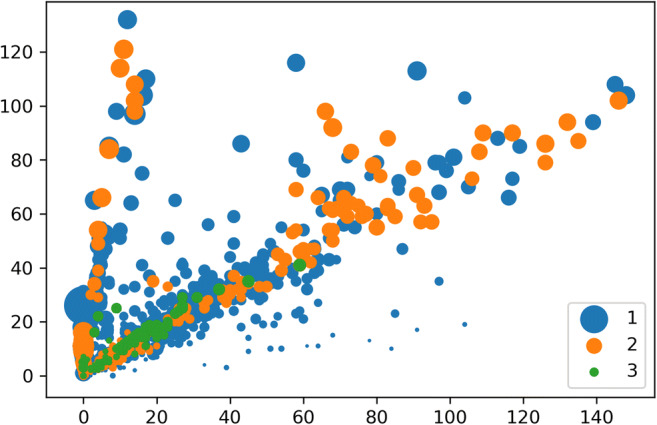
Re-sampled data loaded for the experiment (1 = adenocarcinoma, 2 = squamous cell carcinoma, 3 = NOS)
Fig. 5.
Structure of a CNN having an architecture similar to the proposed CNN-BiRNN model
Result
In the first phase of the experiment, the best model was found at epoch 413 of iteration 6 while executing the single CNN-BiRNN model. The highest test accuracy achieved was 92.59% (the training accuracy was 81.06%). In the ensemble of CNN-BiRNN, the highest test accuracy was 96.29% found at epoch 450 of iteration 3 (the training accuracy was 85.18%). The test accuracy of a CNN model having similar architecture had 90% test accuracy with a training accuracy of 93% (epoch 492). The comparison of the best models found during the experiment was recorded in Table 1.
Table 1.
Evaluation of different best models found
| Model | Accuracy | Precision | Recall | F1-score | Cohen’s kappa | ROC AUC |
|---|---|---|---|---|---|---|
| Ensemble CNN+BiRNN | 96.29 | 96.29 | 96.09 | 96.67 | 93.61 | 98.88 |
| Single CNN+BiRNN | 92.59 | 92.59 | 92.05 | 92.49 | 86.95 | 96.67 |
| CNN | 90.00 | 90.00 | 90.00 | 90.01 | 82.65 | 95.92 |
The average result depicted by the ensemble CNN-BiRNN model was recorded in Table 2.
Table 2.
Average results of the proposed model observed after the 10th iteration of the experiment
| Parameter | Mean with standard deviation |
|---|---|
| Validation accuracy | 94.42 ± 0.005 |
| Cohen’s kappa statistics | 89.22 ± 0.009 |
| ROC-AUC score | 98.47 ± 0.005 |
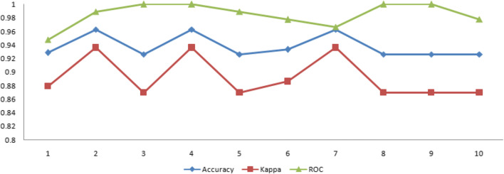
The evolution of the experiment conducted was also observed by using evaluative metrics like training and validation loss, training and validation accuracy, kappa and ROC-AUC (receiver operating curve–area under curve) score (Fig. 6).
Fig. 6.
Iteration wise result of the experiment carried out with CNN-BiRNN ensemble
Discussion
After comparing Tables 1 and 2, the average results achieved by the proposed model ensemble were found far better than the best scores got by the single model or the CNN model. The AUC performance was also convincing than the results got by the contemporary studies discussed in the “Related Work” section. The iteration-wise performance of the model was also found consistent (Fig. 6). The training and validation curve of the single model (Fig. 7) showed that training loss was less than the validation loss, and training accuracy was more than the validation accuracy. The training and validation curve of the model ensemble (Fig. 8) showed that validation accuracy was higher than the training accuracy. Validation accuracy was more because during training, dropout layers were used and some features became zero to minimize overfitting, but during validation all the features were present and thus it showed better accuracy. The overlapping or over-fitting was also less in the model ensemble. These results may draw a conclusion in favor of the proposed model. The model ensemble will definitely be useful in the automated prognosis of NSCLC, and it will also help radiologists and oncologists by acting as a supportive decision-making mechanism.
Fig. 7.
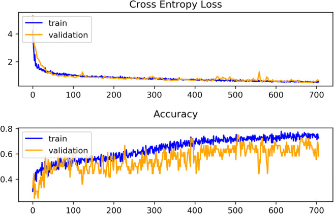
Glimpse of training and validation loss and accuracy observed in the single CNN-BiRNN model
Fig. 8.
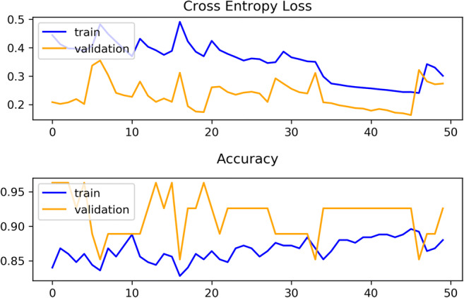
Glimpse of training and validation loss and accuracy observed in the CNN-BiRNN model ensemble
Future Work
The proposed model may be refined further by conducting experiments with varied hyper-parameters, e.g., hidden layers, batch size, and patience in early stopping. Experiments may also be carried out with other similar datasets or by combining other meta-learners with the existing model. These types of evaluative studies will develop the usage of prognostic medical image biomarkers with NSCLC and other types of cancers.
Compliance with Ethical Standards
Conflict of Interest
The authors declare that they have no conflict of interest.
Ethical Approval
For this type of study formal consent is not required.
Informed Consent
Not applicable.
Footnotes
Publisher’s Note
Springer Nature remains neutral with regard to jurisdictional claims in published maps and institutional affiliations.
Contributor Information
Dipanjan Moitra, Email: tataijal@gmail.com.
Rakesh Kumar Mandal, Email: rakesh_mndl@rediffmail.com.
References
- 1.Kerr KM, Bubendorf L, Edelman MJ, Marchetti A, Mok T, Novello S, O'Byrne K, Stahel R, Peters S, Felip E, Members P, Stahel R, Felip E, Peters S, Kerr K, Besse B, Vansteenkiste J, Eberhardt W, Edelman M, Mok T, O'Byrne K, Novello S, Bubendorf L, Marchetti A, Baas P, Reck M, Syrigos K, Paz-Ares L, Smit EF, Meldgaard P, Adjei A, Nicolson M, Crinò L, Van Schil P, Senan S, Faivre-Finn C, Rocco G, Veronesi G, Douillard J-Y, Lim E, Dooms C, Weder W, De Ruysscher D, De Pechoux C, De Leyn P, Westeel V. Second ESMO consensus conference on lung cancer: pathology and molecular biomarkers for non-small-cell lung cancer. Annals of Oncology. 2014;25(9):1681–1690. doi: 10.1093/annonc/mdu145. [DOI] [PubMed] [Google Scholar]
- 2.Wu Weimiao, Parmar Chintan, Grossmann Patrick, Quackenbush John, Lambin Philippe, Bussink Johan, Mak Raymond, Aerts Hugo J. W. L., Exploratory study to identify radiomics classifiers for lung cancer histology, Frontiers in Oncology, Volume 6, 2016, 10.3389/fonc.2016.00071 [DOI] [PMC free article] [PubMed]
- 3.Wilkerson MD, Schallheim JM, Hayes DN, Roberts PJ, Bastien RRL, Mullins M, Yin X, Miller CR, Thorne LB, Geiersbach KB, Muldrew KL, Funkhouser WK, Fan C, Hayward MC, Bayer S, Perou CM, Bernard PS. Prediction of lung cancer histological types by RT-qPCR gene expression in FFPE specimens. The Journal of Molecular Diagnostics. 2013;15(4):485–497. doi: 10.1016/j.jmoldx.2013.03.007. [DOI] [PMC free article] [PubMed] [Google Scholar]
- 4.A. Karlsson, H. Cirenajwis, K. Ericson-Lindqvist, C. Reuterswärd, M. Jönsson, A. Patthey, A.F. Behndig, M. Johansson, M. Planck, J. Staaf, 19P Single sample predictor of non-small cell lung cancer histology based on gene expression analysis of archival tissue, Journal of Thoracic Oncology, Volume 13, Issue 4
- 5.Travis WD, Brambilla E, Geisinger KR. Histological grading in lung cancer: One system for all or separate systems for each histological type? European Respiratory Journal. 2016;47(3):720–723. doi: 10.1183/13993003.00035-2016. [DOI] [PubMed] [Google Scholar]
- 6.Visser S, Hou J, Bezemer K, de Vogel LL, Hegmans JPJJ, Stricker BH, Philipsen S, Aerts JGJV. Prediction of response to pemetrexed in non-small-cell lung cancer with immunohistochemical phenotyping based on gene expression profiles. BMC Cancer. 2019;19:440. doi: 10.1186/s12885-019-5645-x. [DOI] [PMC free article] [PubMed] [Google Scholar]
- 7.Hou J, Aerts J, den Hamer B, van IJcken W, den Bakker M, Riegman P, van der Leest C, van der Spek P, Foekens JA, Hoogsteden HC, Grosveld F, Philipsen S. Gene expression-based classification of non-small cell lung carcinomas and survival prediction. PLoS ONE. 2010;5(4):e10312. doi: 10.1371/journal.pone.0010312. [DOI] [PMC free article] [PubMed] [Google Scholar]
- 8.Mobadersany P, Yousefi S, Amgad M, Gutman DA, Barnholtz-Sloan JS, Velázquez JE, Vega DJ, Brat L, Cooper AD. Predicting cancer outcomes from histology and genomics using convolutional networks. Proceedings of the National Academy of Sciences Mar. 2018;115(13):E2970–E2979. doi: 10.1073/pnas.1717139115. [DOI] [PMC free article] [PubMed] [Google Scholar]
- 9.N. Zhang, J. Wu, M. Yang, J. Yu, R. Li, A composite model integrating imaging, histological, and genetic features to predict tumor mutation burden in non-small cell lung cancer patients, International Journal of Radiation Oncology Biology Physics, Volume 105, Issue 1, 2019
- 10.Digumarthy SR, Padole AM, Gullo RL, Sequist LV, Kalra MK. Can CT radiomic analysis in NSCLC predict histology and EGFR mutation status? Medicine (Baltimore) 2019;98(1):e13963. doi: 10.1097/MD.0000000000013963. [DOI] [PMC free article] [PubMed] [Google Scholar]
- 11.Karlsson A, Cirenajwis H, Ericson-Lindquist K, Brunnström H, Reuterswärd C, Jönsson M, Ortiz-Villalón C, Hussein A, Bergman B, Vikström A, Monsef N, Branden E, Koyi H, de Petris L, Micke P, Patthey A, Behndig AF, Johansson M, Planck M, Staaf J. A combined gene expression tool for parallel histological prediction and gene fusion detection in non-small cell lung cancer. Scientific Reports. 2019;9:5207. doi: 10.1038/s41598-019-41585-4. [DOI] [PMC free article] [PubMed] [Google Scholar]
- 12.Tafadzwa Lawrence Chaunzwa, David C. Christiani, Michael Lanuti, Andrea Shafer, Nancy Diao, Raymond H. Mak, Hugo Aerts, Using deep-learning radiomics to predict lung cancer histology, Journal of Clinical Oncology 36, no. 15_suppl (2018), DOI: 10.1200/JCO.2018.36.15_suppl.8545
- 13.Wu Weimiao, Parmar Chintan, Grossmann Patrick, Quackenbush John, Lambin Philippe, Bussink Johan, Mak Raymond, Aerts Hugo J. W. L., Exploratory study to identify radiomics classifiers for lung cancer histology, Frontiers in Oncology, Vol. 6, 2016, DOI=10.3389/fonc.2016.00071 [DOI] [PMC free article] [PubMed]
- 14.He B, Zhao W, Pi J-Y, Han D, Jiang Y-M, Zhang Z-G, Zhao W. A biomarker basing on radiomics for the prediction of overall survival in non–small cell lung cancer patients. Respir Res. 2018;19:199. doi: 10.1186/s12931-018-0887-8. [DOI] [PMC free article] [PubMed] [Google Scholar]
- 15.Coudray N, Ocampo PS, Sakellaropoulos T, Narula N, Snuderl M, Fenyö D, Moreira AL, Razavian N, Tsirigos A. Classification and mutation prediction from non–small cell lung cancer histopathology images using deep learning. Nat Med. 2018;24:1559–1567. doi: 10.1038/s41591-018-0177-5. [DOI] [PMC free article] [PubMed] [Google Scholar]
- 16.Wang X, Mao K, Wang L, Yang P, Lu D, He P. An appraisal of lung nodules automatic classification algorithms for CT images. Sensors (Basel) 2019;19(1):E194. doi: 10.3390/s19010194. [DOI] [PMC free article] [PubMed] [Google Scholar]
- 17.Clark K, Vendt B, Smith K, Freymann J, Kirby J, Koppel P, Moore S, Phillips S, Maffitt D, Pringle M, Tarbox L, Prior F. The Cancer Imaging Archive (TCIA): maintaining and operating a public information repository. Journal of Digital Imaging. 2013;26(Number 6):1045–1057. doi: 10.1007/s10278-013-9622-7. [DOI] [PMC free article] [PubMed] [Google Scholar]
- 18.Gevaert O, Xu J, Hoang CD, Leung AN, Xu Y, Quon A, Rubin DL, Napel S, Plevritis SK. Non–small cell lung cancer: identifying prognostic imaging biomarkers by leveraging public gene expression microarray data—methods and preliminary results. Radiology. Radiological Society of North America (RSNA). 2012;264:387–396. doi: 10.1148/radiol.12111607. [DOI] [PMC free article] [PubMed] [Google Scholar]
- 19.Moitra D, Mandal RK. Automated grading of non-small cell lung cancer by fuzzy rough nearest neighbour method. Netw Model Anal Health Inform Bioinforma. 2019;8:24. doi: 10.1007/s13721-019-0204-6. [DOI] [Google Scholar]
- 20.Zhiyong Cui, Ruimin Ke, Yinhai Wang. Deep bidirectional and unidirectional LSTM recurrent neural network for network-wide traffic speed prediction. arXiv:1801.02143
- 21.Xingjian Shi, Zhourong Chen, Hao Wang, Dit-Yan Yeung, Wai-kin Wong, Wang-chun Woo. Convolutional LSTM network: a machine learning approach for precipitation nowcasting. arXiv:1506.04214
- 22.Jeff Donahue, Lisa Anne Hendricks, Marcus Rohrbach, Subhashini Venugopalan, Sergio Guadarrama, Kate Saenko, Trevor Darrell. Long-term recurrent convolutional networks for visual recognition and description. arXiv:1411.4389 [DOI] [PubMed]
- 23.Moitra D, Mandal RK. Automated AJCC (7th edition) staging of non-small cell lung cancer (NSCLC) using deep convolutional neural network (CNN) and recurrent neural network (RNN) Health Inf Sci Syst. 2019;7:14. doi: 10.1007/s13755-019-0077-1. [DOI] [PMC free article] [PubMed] [Google Scholar]
- 24.Bakr, Shaimaa; Gevaert, Olivier; Echegaray, Sebastian; Ayers, Kelsey; Zhou, Mu; Shafiq, Majid; Zheng, Hong; Zhang, Weiruo; Leung, Ann; Kadoch, Michael; Shrager, Joseph; Quon, Andrew; Rubin, Daniel; Plevritis, Sylvia; Napel, Sandy. (2017). Data for NSCLC Radiogenomics collection. The Cancer Imaging Archive. 10.7937/K9/TCIA.2017.7hs46erv
- 25.D. Moitra, R. Mandal, Review of brain tumor detection using pattern recognition techniques, International Journal of Computer Sciences and Engineering, Vol. 5, Issue 2, pp. 121–123, 2017
- 26.D. Moitra, Comparison of multimodal tumor image segmentation techniques, International Journal of Advanced Research in Computer Science, Volume 9, No. 3, 2018, 10.26483/ijarcs.v9i3.6010
- 27.D. Moitra, R. Mandal, Segmentation strategy of PET brain tumor image, Indian Journal of Computer Science and Engineering, Vol. 8 No. 5 2017, e-ISSN:0976–5166
- 28.H. M. Nguyen, E. W. Cooper, K. Kamei, Borderline over-sampling for imbalanced data classification, International Journal of Knowledge Engineering and Soft Data Paradigms, 3(1), pp.4–21, 2009
- 29.François Chollet, Deep learning with Python, Manning Publications Co., 2018, ISBN 9781617294433
- 30.Powers DMW. [2007], Evaluation: from precision, recall and F-measure to ROC, informedness, markedness & correlation. Journal of Machine Learning Technologies. 2011;2(1):37–63. [Google Scholar]
- 31.Hochreiter S, Schmidhuber J. Long short-term memory. Neural Computation. 1997;9(8):1735–1780. doi: 10.1162/neco.1997.9.8.1735. [DOI] [PubMed] [Google Scholar]
- 32.Dipanjan Moitra, Classification of malignant tumors: a practical approach, LAP LAMBERT Academic Publishing, 2019, ISBN: 978-613-9-47500-1
- 33.Dipanjan Moitra, R. K. Samanta, Performance evaluation of BioPerl, Biojava, BioPython, BioRuby and BioSmalltalk for executing bioinformatics tasks, International Journal of Computer Sciences and Engineering, Vol.03, Issue.01, pp.157–164, 2015
- 34.AJCC Cancer Stating Manual 7th Edition, American Joint Committee on Cancer, ISBN 978-0-387-88440-0, Springer New York


