Training and Validation of Deep Neural Networks for the Prediction of 90-Day Post-Liver Transplant Mortality Using UNOS Registry Data

Abstract

Prediction models of post-liver transplant mortality are crucial so that donor organs are not allocated to recipients with unreasonably high probabilities of mortality. Machine learning algorithms, particularly deep neural networks (DNNs), can often achieve higher predictive performance than conventional models. In this study, we trained a DNN to predict 90-day post-transplant mortality using preoperative variables and compared the performance to that of the Survival Outcomes Following Liver Transplantation (SOFT) and Balance of Risk (BAR) scores, using United Network of Organ Sharing data on adult patients who received a deceased donor liver transplant between 2005 and 2015 (n = 57,544). The DNN was trained using 202 features, and the best DNN’s architecture consisted of 5 hidden layers with 110 neurons each. The area under the receiver operating characteristics curve (AUC) of the best DNN model was 0.703 (95% CI: 0.682-0.726) as compared to 0.655 (95% CI: 0.633-0.678) and 0.688 (95% CI: 0.667-0.711) for the BAR score and SOFT score, respectively. In conclusion, despite the complexity of DNN, it did not achieve a significantly higher discriminative performance than the SOFT score. Future risk models will likely benefit from the inclusion of other data sources, including high-resolution clinical features for which DNNs are particularly apt to outperform conventional statistical methods.

LIVER transplantation is the definitive treatment for irreversible liver failure, with thousands of lives saved each year in the Unites States through deceased donor organ donation. Unfortunately, with the demand for donor organs far exceeding the supply, thousands of patients die waiting for this life saving procedure [1]. As such, the development of predictive models of post-transplant mortality is crucial to avoid transplanting an individual with an unacceptably low probability of post-transplant survival. As the severity of recipient medical comorbidities has grown, there is concern that an increasing number of patients are becoming too sick to transplant [2,3]. While the prediction of preoperative mortality among those waiting for an organ has been quite successful with the adoption of the Model for End-Stage Liver Disease (MELD) score to prioritize organ allocation [3-6], the accurate prediction of post-transplant mortality has been difficult and less successful [7].

Several predictive models have been developed using preoperative recipient and organ donor factors from either registry- or institution-level data. These have been developed with the aim of avoiding futile transplantation, assisting with donor-recipient matching, and for comparing outcomes across different institutions. Two of the most commonly cited risk models are the Balance of Risk (BAR) score [8] and the Survival Outcomes Following Liver Transplantation (SOFT) score [9], both of which predict 90-day post-liver transplant mortality using United Network of Organ Sharing (UNOS) registry data. The SOFT score incorporated a combination of 18 recipient and donor variables and achieved a c-statistic of 0.7, and the BAR score achieved a C-statistic of 0.7 using a combination of just 6 recipient and donor variables. Despite the popularity of these models in academic circles, their clinical use has been limited due to their modest discriminative performance with decision making left to the judgment of the selection committee and transplant clinicians.

Risk models in medicine have traditionally been based on regression models whereby the outcome variable is modeled as a linear combination of predictor variables and thereby have been limited in their ability to model high-order interactions and nonlinear functions of the features. Machine learning algorithms, which allow for more flexible modeling of the data, can often achieve higher predictive performance than more conventional statistical models. One class of machine learning algorithms, deep neural networks (DNNs), also known as deep learning, has become popular in recent years because of its success in solving a variety of problems from computer vision [10-15], high energy physics [16,17], chemistry [18-20], and biology [21-23]. In clinical medicine, predictive modeling using machine learning has been applied to the prediction of cardiorespiratory instability [24,25], 30-day readmission, [26,27], and in-hospital postoperative mortality [28].

The use of DNNs in liver transplantation has been relatively limited. To date, DNNs have been largely unexplored in the prediction of post-liver transplant mortality using UNOS data. In this manuscript, we present the development and validation of a DNN model using preoperative variables from the UNOS registry to predict 90-day post-liver transplant mortality. We compare the discriminative ability of the DNN model to that of the BAR and SOFT score models.

MATERIALS AND METHODS

This manuscript follows the “Guidelines for Developing and Reporting Machine Learning Predictive Models in Biomedical Research: A Multidisciplinary View” [29].

UNOS Data Extraction

All data for this study were extracted from the standard transplant analysis and research (STAR) dataset, which contains patient-level data for all transplants in the Unites States reported to the Organ Procurement and Transplantation Network (OPTN) since October 1, 1989. The database has been used in numerous important studies of transplantation [30] and contains data on pretransplant variables pertaining to the recipient, donor variables reported from the organ procurement organization, as well as post-transplantation outcome data. The OPTN mortality data are linked by UNOS to the Social Security Death Master file to improve ascertainment of recipient death data [30]. In accordance with the OPTN Final Rule, 42 CFR Part 121, the UNOS provided the author (B.E.) with the patient-level, nonidentifiable data extracted from the STAR database maintained by UNOS for the purpose of conducting this research. Access to this data was approved through a data-use agreement with UNOS.

Study Sample

The study sample included adult deceased donor liver transplants performed from 2005 to 2015. Transplants performed from 2016 onward were not included in this analysis to ensure adequate time for ascertainment of outcome data, and transplants performed prior to 2005 were excluded because 1. transplants before 2002 were performed prior to implementation of the MELD score allocation system and 2. data on several predictor variables were either not reported or were inconsistently recorded prior to that time. Exclusion criteria included age less than 18 years, living donor transplantation (n = 2347), multiple-organ transplantation (n = 5267), as well as those lost to follow-up within 90 days post-transplantation (n = 70) as these cases were excluded in the development of the SOFT score and BAR score (Fig 1). For patients who underwent more than 1 liver transplantation (n = 3503), we included each of the transplantations in the analysis, as did other comparable prediction models. The study sample included split liver as well as donation after cardiac death donors. In sum, we analyzed 57,544 recipients.

Fig 1.

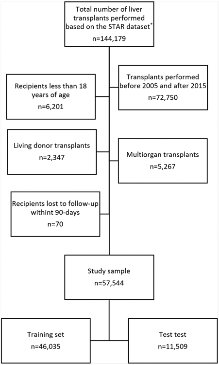
Flow chart of study cohort. The flow chart illustrates the inclusion and exclusion criteria of liver transplant recipients included in the study sample. STAR, Standard Transplant Analysis and Research. *Based on OPTN data as of September 9, 2016.

Model Endpoint Definition

The occurrence of death within 90 days from transplantation was extracted as a binary event (0, 1). An event occurred if the value of the variable “pstatus” from the STAR dataset was equal to “1”, and the variable “prime” was less than or equal to 90. The variable “pstatus” indicates whether the recipient had died post-transplant, and the variable “ptime” indicates the time from transplantation to either death or censoring. These variables are based on the combination of mortality data from OPTN database as well as verified external sources of death (described above) and not based on the variable “PX_STAT,” which only accounts for death as documented by the OPTN alone.

Model Input Features

The original STAR dataset contained 395 variables, many of which were not considered for inclusion in the model. Variables that were excluded from model development included those pertaining to post-transplant data, living donor transplants, multiorgan transplants, and identifier code variables. Variables with zero or near zero variances, high levels of missing data (> 98%) or those that were highly correlated to other variables (r > 0.99) were removed. A few variables with > 50% missing data combined with low clinical significance based on domain experts (B.E. and C.W.) were not analyzed. This resulted in 202 features, including 132 recipient variables and 70 donor-related variables (Table 1). To further reduce the feature set, variables with greater than 50% missing data or those containing greater than 95% zero values were removed, and the remaining variables comprised a reduced feature set (RFS).

Table 1.

Description of Deep Neural Network Input Features

Feature	Description
abo_A†	Recipient blood type A
abo_AB	Recipient blood type AB
abo_B	Recipient blood type B
abo_don_A	Donor blood type A
abo_don_AB†	Donor blood type AB
abo_don_B	Donor blood type B
abo_don_O	Donor blood type O
abo_mat	Donor-recipient ABO match level
abo_O	Recipient blood type O
age	Recipient’s age
age_don	Donor’s age
albumin_tx	Recipient’s albumin concentration at transplant
antihype_don	Donor received antihypertensives within 24 h of cross clamp
arginine_don	Donor received arginine vasopressin within 24 h of cross clamp
ascites_tx*	Recipient’s degree of ascites at transplantation
bact_perit_tcr	Recipient had history of SBP at registration
bmi_calc	Recipient’s BMI at transplantation
bmi_don_calc	Donor’s BMI
bmi_tcr	Recipient’s BMI at registration
bun_don	Donor’s terminal blood urea nitrogen concentration
cardarrest_neuro	Donor had a cardiac arrest after brain death
cdc_risk_hiv_don	Donor had risk factors for blood-borne disease transition
citizenship†,*	Recipient was a United States citizen
citizenship_don†,*	Donor was a United States citizen
clin_infect_don	Donor had a clinical infection
cmv_don*	Donor’s CMV seropositivity
cmv_igg*	Recipient’s CMV IGG test result at transplant
cmv_igm‡,*	Recipient’s CMV IGM test result at transplant
cmv_status*	Recipient’s CMV seropositivity at transplant
cod_cad_don_1	Donor’s cause of death was due to anoxia
cod_cad_don_2	Donor’s cause of death was due to stroke
cod_cad_don_3	Donor’s cause of death was due to head trauma
cod_cad_don_4†	Donor’s cause of death was due to a cans tumor
cold_isch	Cold ischemia time
coronary1*	Donor coronary angiogram was performed, and result was normal
creat_don	Donor’s terminal creatinine concentration
creat_tx	Recipient’s creatinine concentration at transplant
dayswait_chron	Number of days recipient was on transplant waiting list
ddavp_don	Donor received DDAVP
death_circum_don*	Donor’s circumstance of death was due to natural causes
death_mech_don†,*	Donor’s mechanism of death
dgn_tcr_AHN†,*	Recipient’s primary diagnosis at listing: acute hepatic necrosis
dgn_tcr_autoimmune†,*	Recipient’s primary diagnosis at listing: autoimmune hepatitis
dgn_tcr_cryptogenic*	Recipient’s primary diagnosis at listing: cryptogenic cirrhosis
dgn_tcr_etoh*	Recipient’s primary diagnosis at listing: ETOH cirrhosis
dgn_tcr_etoh_hcv*	Recipient’s primary diagnosis at listing: ETOH or HCV cirrhosis
dgn_tcr_HBV†,*	Recipient’s primary diagnosis at listing: HBV cirrhosis
dgn_tcr_HCC*	Recipient’s primary diagnosis at listing: HCC cirrhosis
dgn_tcr_HCV*	Recipient primary diagnosis at listing: HCV cirrhosis
dgn_tcr_NASH*	Recipient’s primary diagnosis at listing: NASH cirrhosis
dgn_tcr_PBC†,*	Recipient’s primary diagnosis at listing: PBC cirrhosis
dgn_tcr_PSC†,*	Recipient’s primary diagnosis at listing: PSC cirrhosis
dgn2_tcr_AHN†,*	Recipient secondary diagnosis at listing: acute hepatic necrosis
dgn2_tcr_autoimmune†,*	Recipient’s secondary diagnosis at listing: autoimmune hepatitis
dgn2_tcr_cryptogenic†,*	Recipient’s secondary diagnosis at listing: cryptogenic cirrhosis
dgn2_tcr_etoh†,*	Recipient’s secondary diagnosis at listing: ETOH cirrhosis
dgn2_tcr_etoh_hcv†,*	Recipient’s secondary diagnosis at listing: ETOH or HCV cirrhosis
dgn2_tcr_HBV†,*	Recipient’s secondary diagnosis at listing: HBV cirrhosis
dgn2_tcr_HCC*	Recipient’s secondary diagnosis at listing: HCC cirrhosis
dgn2_tcr_HCV†,*	Recipient’s secondary diagnosis at listing: HCV cirrhosis
dgn2_tcr_NASH†,*	Recipient’s secondary diagnosis at listing: NASH cirrhosis
dgn2_tcr_PBC†,*	Recipient’s secondary diagnosis at listing: PBC cirrhosis
dgn2_tcr_PSC†,*	Recipient’s secondary diagnosis at listing: PSC cirrhosis
diab*	Recipient had diabetes at registration
diabdur_don	Duration of time that donor had diabetes
diabetes_don	Donor had a history of diabetes
diag_AHN†,*	Recipient’s diagnosis at transplant: acute hepatic necrosis
diag_autoimmune†,*	Recipient’s diagnosis at transplant: autoimmune hepatitis
diag_cryptogenic†,*	Recipient’s diagnosis at transplant: cryptogenic cirrhosis
diag_etoh*	Recipient’s diagnosis at transplant: ETOH cirrhosis
diag_etoh_hcv†,*	Recipient’s diagnosis at transplant: ETOH or HCV cirrhosis
diag_HBV†,*	Recipient’s diagnosis at transplant: HBV cirrhosis
diag_HCC*	Recipient’s diagnosis at transplant: HCC cirrhosis
diag_HCV*	Recipient’s diagnosis at transplant: HCV cirrhosis
diag_NASH*	Recipient’s diagnosis at transplant: NASH cirrhosis
diag_PBC†,*	Recipient’s diagnosis at transplant: PBC cirrhosis
diag_PSC†,*	Recipient’s diagnosis at transplant: PSC cirrhosis
dial_tx	Recipient had dialysis in the wk prior to transplant
distance	Distance from donor hospital to transplant hospital
ebv_igg_cad_don*	Donor’s EBV IGG test result
ebv_igm_cad_don†,*	Donor’s EBV IGM test result
ebv_serostatus*	Recipient’s EBV seropositivity at transplant
ecd_donor	Donor was an ECD donor per kidney allocation definition
education*	Recipient’s highest education level at registration
enceph_tx*	Recipient’s degree of encephalopathy at transplant
end_stat†,*	Recipient was status 1 at time of transplant
ethcat_1*	Recipient’s race is Caucasian
ethcat_2*	Recipient’s race is of African descent
ethcat_4*	Recipient’s ethnicity is Hispanic
ethcat_5†,*	Recipient’s race is Asian
ethcat_don_1*	Donor’s race is Caucasian
ethcat_don_2*	Donor’s race is of African descent
ethcat_don_4*	Donor’s ethnicity is Hispanic
ethcat_don_5†,*	Donor’s race is Asian
ethcat_don_other†,*	Donor’s race is other
ethcat_other†,*	Recipient’s race is other
ever_approved‡	Recipient ever had a MELD exception application approved
exc_case	Recipient had MELD exception points at the time of transplantation
exc_diag_id_cat1*	Recipient’s exception points allotted for HCC
exc_diag_id_cat2†,*	Recipient’s exception points allotted for familial amyloidosis
exc_diag_id_cat3†,*	Recipient’s exception points allotted for hepatopulmonary syndrome
exc_diag_id_cat4†,*	Recipient’s exception points allotted for portopulmonary hypertension
exc_diag_id_cat5†,*	Recipient’s exception points allotted for metabolic diseases
exc_diag_id_cat6†,*	Recipient’s exception points allotted for hepatic artery thrombosis
exc_diag_id_cat7*	Recipient’s exception points allotted for other causes
exc_ever	Whether an exception was ever submitted for the recipient
exc_hcc	Recipient’s exception was for HCC
final_inr	Recipient’s INR at transplantation
final_serum_sodium	Recipient’s sodium concentration at transplantation
func_stat_tcr*	Recipient’s functional status at registration
func_stat_trr*	Recipient’s functional status at transplantation
gender	Recipient’s gender
gender_don	Donor’s gender
hbv_core*	Recipient’s HBV core seropositivity
hbv_core_don*	Donor’s HBV core seropositivity
hbv_sur_antigen†,*	Recipient’s HBV surface antigen seropositivity
hbv_sur_antigen_don†,*	Donor’s HBV surface antigen seropositivity
hcc_ever_appr‡	Whether recipient ever had an approved HCC exception
hcv_serostatus	Recipient’s HCV seropositivity
hematocrit_don	Donor’s hematocrit
hep_c_anti_don†	Donor’s HCV seropositivity
heparin_don	Donor received heparin
hgt_cm_calc	Recipient’s height at transplantation
hgt_cm_don_calc	Donor’s height
hgt_cm_tcr	Recipient’s height at registration
hist_cancer_don†	Donor had a history of cancer
hist_cig_don	Donor had a history > 20 pack-years of smoking
hist_cocaine_don	Donor had a history of cocaine use
hist_insulin_dep_don‡	Donor had a history of insulin dependent diabetes
hist_oth_drug_don	Donor had a history of other drug use in the past
history_mi_don†	Donor had a history of myocardial infarction
hypertens_dur_don*	Donor’s history and duration of hypertension
index2*	Recipient’s number of previous liver transplants prior to current one
init_age	Recipient’s age at listing
init_albumin*	Recipient’s albumin concentration at listing
init_ascites	Recipient’s degree of ascites at listing
init_bilirubin	Recipient’s bilirubin concentration at listing
init_bmi_calc	Recipient’s BMI at listing
init_dialysis_prior_week†	Recipient at listing had received dialysis twice in the prior wk
init_enceph*	Recipient’s degree of encephalopathy at listing
init_hgt_cm	Recipient’s height at listing
init_inr	Recipient’s INR at listing
init_meld_peld_lab_score	Recipient’s laboratory MELD score at listing
init_serum_creat	Recipient’s creatinine concentration at listing
init_serum_sodium	Recipient’s sodium concentration at listing
init_stat†,*	Recipient was status 1 at listing
init_wgt_kg	Recipient’s weight at listing
inotrop_support_don	Donor was on inotropic medications at procurement
inr_tx	Recipient’s INR at transplantation
insulin_dep_don*	Donor had a history of insulin dependent diabetes
insulin_don	Recipient received insulin within 24 h of cross clamp
life_sup_tcr†	Recipient was on “life support” at registration
life_sup_trr	Recipient was on “life support” at transplant
lityp*	Donor graft was a split or whole graft
macro_fat_li_don*	Donor organ was biopsied and macrosteatosis was greater than 30%
Malig	Recipient had a history of malignancy at transplantation
malig_tcr	Recipient had a history of malignancy at registration
malig_type†,‡	Recipient’s malignancy type was HCC
med_cond_trr	Recipient’s medical condition at transplant (1 = home, 2 = hospital, 3 = ICU)
meld_diff_reason_cd_1†,*	MELD score and laboratory MELD score difference is because of status 1
meld_diff_reason_cd_2*	MELD score and laboratory MELD score difference is because of HCC
meld_peld_lab_score	Recipient’s laboratory MELD score at transplant
micro_fat_li_don*	Donor organ was biopsied and microsteatosis was greater than 30%
non_hrt_don	Donor is a donation after cardiac death organ
num_prev_tx	Recipient’s number of previous transplants
on_vent_trr	Recipient was on ventilator at time of transplant
oth_life_sup_tcr†	Recipient was on other type of “life support” at registration
oth_life_sup_trr†	Recipient was on other type of “life support” at transplantation
ph_don	Donor pH
portal_vein_tcr†	Recipient had portal vein thrombosis at registration
portal_vein_trr	Recipient had portal vein thrombosis at transplant
prev_ab_surg_tcr	Recipient had previous abdominal surgeries at registration
prev_ab_surg_trr	Recipient had previous abdominal surgeries at transplant
prev_tx	Recipient ever had a previous liver transplant
pri_payment_tcr	Projected payment for transplant at registration is from private insurance
pri_payment_trr*	Payment source for transplant is from private insurance
protein_urine	Donor had protein in urine
prvtxdif*	Number of days between current liver transplant and prior liver transplant
pt_diuretics_don	Donor received diuretics within 24 h of procurement
pt_oth_don	Donor received prerecovery medications
pt_steroids_don	Donor received steroids within 24 h of procurement
pt_t3_don†	Donor received T3 within 24 h of procurement
pt_t4_don	Donor received T4 within 24 h of procurement
recov_out_us†	Donor organ was recovered outside of the United States
resuscit_dur*	Time from cardiac arrest to resuscitation for brain dead donors with arrest
sgot_don	Donor’s terminal AST concentration
sgpt_don	Donor’s terminal ALT concentration
share_ty†,*	Donor’s allocation type (local/regional/other)
tattoos	Donor had tattoos
tbili_don	Donor’s terminal bilirubin concentration
tbili_tx	Recipient’s bilirubin concentration at transplant
tipss_tcr	Recipient had a TIPS at registration
tipss_trr	Recipient had a TIPS at time of transplant
vasodil_don	Donor received vasodilators within 24 h of cross clamp
vdrl_don†	Donor’s RPR seropositivity
ventilator_tcr†	Recipient was on ventilator at registration
warmjsch_tm_don†,*	Duration of warm ischemia time for DCD donors
wgt_kg_calc	Recipient’s weight at transplant
wgt_kg_don_calc	Donor’s weight
wgt_kg_tcr	Recipient’s weight at registration
work_income_tcr	Recipient was working for income at registration
work_income_trr	Recipient was working for income at time of transplantation

Abbreviations: ALT, alanine aminotransferase; AST, aspartate aminotransferase; BMI, body mass index; CMV, cytomegalovirus virus; DCD, donation after cardiac death; DDAVP, desmopressin; EBV, Epstein-Barr virus; ECD, expanded criteria donor; ETOH, alcoholic; HBV, hepatitis B virus; HCC, hepatocellular carcinoma; HCV, hepatitis C virus; ICU, intensive care unit; IGM, Immunoglobulin M; IGG, Immunoglobulin G; INR, international normalized ratio; MELD, Model for End-Stage Liver Disease; NASH, nonalcoholic steatohepatitis; PBC, primary biliary cirrhosis; PSC, primary sclerosing cholangitis; RPR, rapid plasma regain; SBP, spontaneous bacterial peritonitis; TIPS, transjugular intrahepatic portosystemic shunt.

^*Input feature was engineered; see Supplemental Table 1 for description.

^†feature excluded from RFS due to greater than 95% of values were equal to zero.

^‡Feature excluded from RFS due to greater than 50% of values were missing.

While most of the categorical features had a simple binary encoding (Table 1), categorical features identified by domain expert (B.E. and C.W.) that required more complex encoding were encoded based on clinician judgment. For example, the variable “DIAG,” which indicates a recipient’s primary liver disease diagnosis at transplantation, contains 70 possible unique diagnosis codes. Rather than creating 70 new binary categorical features, groups of diagnosis codes were used to collapse the 70 unique codes into 11 new categorical features.

BAR Score and SOFT Score

The BAR score and SOFT score are 2 models used to predict 90-day post-liver transplant survival using UNOS data. To compare the discriminative ability of the DNN to that of these models, the BAR score and SOFT score were calculated for recipients in this dataset. The formula for calculating the BAR score and SOFT score are provided in Fig 2 [8,9]. Data on cold ischemia time was missing for 2.8% of recipients; therefore, the BAR score could not be calculated for these subjects. The amount of missing data for other variables was < 0.1%, and these cases were removed from the calculation of the BAR score’s area under the receiver operating characteristics curve (AUC). Missing data for the SOFT score was handled by assigning the missing value to the reference group category, as indicated by the scoring methodology. One of the 18 variables that comprises the original SOFT score is the presence of a portal bleed within 48 hours of transplantation. This variable was not available in the STAR dataset and therefore was not included in the calculated SOFT score. In the original development of the SOFT score model, only 3% of patients had a portal bleed, and data for this variable were missing for 50% of recipients [9]. In our analysis, we calculated the SOFT score using the remaining 17 components.

Fig 2.

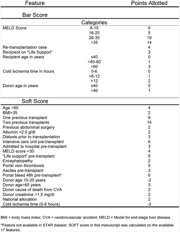
Calculation of BAR score and SOFT score. The BAR score and SOFT score are calculated by adding the points assigned to each attribute. BMI, body mass index; CVA, cerebrovascular accident; MELD, Model for end-stage liver disease. *Feature not available in STAR dataset. SOFT score in this manuscript was calculated on the available 17 features.

Data Preprocessing

Prior to model development, missing values were imputed with the mean value for continuous variables and with 0 for categorical variables. The data were then randomly divided into training (80%) and test (20%) data sets. The training data was rescaled to have a mean of 0 and standard deviation of 1 per feature. The test data was rescaled to the training mean and standard deviation.

“Soft” Binning Features

Besides following the standard approach of normalizing individual input features, we also experimented with a novel idea that we will refer to as “soft binning.” Similar to standard/“hard” binning, the data representation of any feature is replaced by a fixed number of bins, containing numbers between 0 and 1. Ordinary binning discretizes a feature by representing it as a single “1” in 1 bin and zeroes in all other bins, potentially resulting in loss of information and making the classification task harder. “Soft” binning is the most straightforward generalization of binning without loss of information, where 2 bins are assigned values in the range of 0 to 1, which sum to 1. These values encode the fraction to which the feature’s value falls into the given bins. For example, if in standard binning a value would fall exactly on the boundary between 2 bins, then it would instead be represented as 2 neighboring entries of “0.5” in the neighboring bins in “soft” binning. Our motivation for creating “soft” binning was that binning alleviates the burden for the neural network to learn individual features thresholds (ie, “high,” “average,” or “low”) and thus improves classification accuracy.

Development of the Model

The primary aim of the study was to classify recipients with 90-day post-liver transplant mortality using DNNs, also referred to as deep learning. During development of DNNs, there are many unknown model parameters that need to be optimized during training. These model parameters are first initialized and then optimized to decrease the error of the model’s output to correctly classify mortality. The type of DNN used in this study was a feedforward network with fully connected layers and a logistic output. “Fully connected” refers to the fact that all neurons between 2 adjacent layers are fully pairwise connected. A logistic output was chosen so that the output of the model could be interpreted as probability of mortality (0-1). We used stochastic gradient descent with momentum (0.2, 0.5, 0.9) and initial learning rates (0.01, 0.001, 0.1) and a batch size of 500. We also assessed DNN architectures of 1 to 5 hidden layers with (10, 50, 100, 110, 115, 120, 130, 140, 150) neurons per layer and rectified linear unit activation functions. The loss function was cross entropy. To minimize overfitting, we used 3 methods: 1. early stopping with a patience of 10 epochs, 2. L2 weight decay, and 3. dropout [31,32]. We assessed L2 weight penalties of (0.01, 0.001, 0.0001), and dropout was applied to all layers with a probability of (0,0.2, 0.5, 0.9). We used 5-fold cross validation with the training set (80%) to select the best hyperparameters and architecture based on mean cross-validation performance. These best hyperparameters and architecture were then used to train a model on the entire training set (80%) prior to testing final model performance on the separate test set (20%).

Model Performance

All model performances were assessed on 20% of the data held out from training as a test set. Model performance was assessed using AUC and was compared to the BAR score and the SOFT score.

Choosing a Threshold

The F1 score, sensitivity, and specificity were calculated for different thresholds for the DNN, as well as for the BAR score and SOFT score models. The F1 score is a measure of precision and recall, ranging from 0 to 1. It is calculated as $1=2\ast \frac{precision\ast recall}{precision+recall}$ Thresholds that optimized the F1 score were then chosen for each model/score. The minimum thresholds to achieve a sensitivity or specificity of 90% for each model/score were also calculated. Ninety-five percent confidence intervals were calculated for all performance metrics using bootstrapping with 1000 samples.

All DNN models were developed and applied using Keras [33]. All performance metrics were calculated using scikit-learn [34]. Code is available upon reasonable request.

RESULTS

Patient Characteristics

The data consisted of 57,544 liver transplant recipients. These data were split into training (n = 46,035) and test (n = 11,509). The 90-day post-liver transplant mortality in the training and test sets were 5.4% (n = 2483) and 5.6% (n = 640), respectively.

Development of the Model

The best DNN model used the 202 original feature set (OFS) with “softbin” preprocessing of input features (DNN with OFS + softbin). The model consisted of 5 hidden layers of 110 neurons per layer with rectified linear unit activations and a logistic output and was trained with no dropout, an L2 weight decay of 0.001, a learning rate of 0.01, and a momentum of 0.5 (Table 2).

Table 2.

Best Deep Neural Network Hyperparameters for Each Model

	# of Hidden Layers	# of Neurons per Layer	L2 Lambda	Dropout Probability	Learning Rate	Momentum
DNN w/original 202 features (OFS)	5	100	0.001	0.5	0.01	0.5
DNN w/OFS + softbin	5	110	0.001	0	0.01	0.5
DNN w/reduced 140 features (RFS)	5	100	0.001	0.5	0.01	0.5
DNN w/RFS + softbin	5	110	0.001	0	0.01	0.5

Description of the architecture and selected hyperparameters of the trained neural networks.

Abbreviations: DNN, deep neural network; OFS, original feature set; RFS, reduced feature set.

Model Performance

All performance metrics reported below refer to the test dataset.

Area Under the Receiver Operating Characteristics Curves

Receiver operating characteristics curves and AUC results are shown in Fig 3 and Table 3. The best DNN model (DNN with OFS + softbin) had a higher AUC (0.703 [95% CI: 0.682-0.726]) compared to that for the BAR score and SOFT score models (0.655 [95% CI: 0.633-0.678]; 0.688 [95% CI: 0.667-0.711]), respectively, on the 11,207 patients with available BAR scores. In addition, softbin preprocessing of input features improved performance of both the OFS and RFS models. While the best DNN had a significantly higher AUC than the BAR score, the DNN did not achieve a significantly higher AUC than the SOFT score. The DNN with the reduced feature set and softbin preprocessing (DNN with RFS + softbin) performed comparably (AUC 0.702 [95% CI: 0.68-0.725]) to the DNN with OFS + softbin.

Fig 3.

Receiver operating characteristic curves to predict 90-day post-liver transplant mortality. The figure illustrates the receiver operating characteristic curves for the BAR score, SOFT score, and each of the DNN models that were developed.

Table 3.

Area Under the ROC Curve Results With 95% Confidence Intervals for the Test Set (n = 11,509) and on the Test Set With No Null BAR Scores (n = 11,207).

	AUC (95% CI)
	n = 11,509	n = 11,207*
BAR score*	0.655 (0.633-0.678)	0.655 (0.633-0.678)
SOFT score	0.691 (0.671-0.714)	0.688 (0.667-0.711)
DNN w/Original 202 Features Set (OFS)	0.697 (0.678-0.72)	0.695 (0.675-0.717)
DNN w/OFS + softbin	0.708 (0.689-0.73)	0.703 (0.682-0.726)
DNN w/Reduced 140 Features Set (RFS)	0.699 (0.681-0.722)	0.698 (0.679-0.72)
DNN w/RFS + softbin	0.707 (0.688-0.729)	0.702 (0.68-0.725)

^*For the entire test set results, BAR score was calculated on 11,207 test patients.

Choosing a Threshold

For comparison of F1 scores, sensitivity, and specificity at different thresholds, the DNN models were compared to the BAR score and SOFT score models (Table 4). Additionally, for each of the thresholds, the number of correctly and incorrectly classified patients is displayed for all test set patients. As the BAR score could not be calculated on 302 patients in the test set due to missing data, Table 4 provides metrics applied to test sets that contain all patients with available data for the model, as well as to the set of patients for which the BAR scores could be calculated.

Table 4.

F1 Score, Sensitivity, Specificity, and Number of Correctly Identified Patients With 95% Confidence Intervals (CI) for the Test Set (n = 11,509) and on the Test Set With No Null BAR Scores (n = 11,207) for the Thresholds That Maximize F1 Score

ALL Test Patients (n = 11,509)
	Threshold	F1 Score (95% CI)	Sensitivity (95% CI)	Specificity (95% CI)	Precision (95% CI)	# TN	# FP	# FN	# TP
BAR Score*	15	0.179 (0.159-0.2)	0.319 (0.287-0.357)	0.873 (0.867-0.88)	0.124 (0.109-0.141)	9269	1343	405	190
SOFT Score	20	0.223 (0.201-0.247)	0.38 (0.344-0.419)	0.881 (0.874-0.887)	0.158 (0.14-0.177)	9571	1298	397	243
DNN w/OFS	0.092	0.212 (0.19-0.236)	0.348 (0.316-0.385)	0.886 (0.88-0.892)	0.153 (0.135-0.171)	9632	1237	417	223
DNN w/OFS + softbin	0.113	0.22 (0.197-0.246)	0.322 (0.289-0.359)	0.906 (0.9-0.911)	0.167 (0.148-0.188)	9843	1026	434	206
DNN w/RFS	0.095	0.212 (0.19-0.235)	0.358 (0.323-0.397)	0.881 (0.875-0.888)	0.151 (0.133-0.169)	9581	1288	411	229
DNN w/RFS + softbin	0.105	0.221 (0.197-0.245)	0.345 (0.311-0.382)	0.895 (0.889-0.901)	0.162 (0.144-0.182)	9727	1142	419	221
ALL Test Patients w/BAR Score (n = 11,207)
	Threshold	F1 Score (95% CI)	Sensitivity (95% CI)	Specificity (95% CI)	Precision (95% CI)	# TN	# FP	# FN	# TP
BAR Score*	15	0.179 (0.159-0.2)	0.319 (0.287-0.357)	0.873 (0.867-0.88)	0.124 (0.109-0.141)	9269	1343	405	190
SOFT Score	20	0.215 (0.191-0.238)	0.375 (0.336-0.416)	0.881 (0.875-0.888)	0.151 (0.132-0.169)	9354	1258	372	223
DNN w/OFS	0.092	0.206 (0.183-0.231)	0.345 (0.309-0.384)	0.887 (0.882-0.893)	0.147 (0.129-0.165)	9418	1194	390	205
DNN w/OFS + softbin	0.114	0.21 (0.186-0.235)	0.309 (0.274-0.346)	0.908 (0.903-0.913)	0.159 (0.138-0.18)	9638	974	411	184
DNN w/RFS	0.095	0.204 (0.181-0.227)	0.353 (0.315-0.391)	0.882 (0.876-0.888)	0.144 (0.126-0.162)	9361	1251	385	210
DNN w/RFS + softbin	0.105	0.21 (0.187-0.236)	0.334 (0.299-0.372)	0.896 (0.891-0.902)	0.153 (0.135-0.174)	9513	1099	396	199

Performance metrics for all models at the threshold that maximized F1 score. Among the trained DNN models, DNN w/RFS + softbin achieved the highest F1 score.

Abbreviations: DNN, deep neural network; FN, false negative; FP, false positive; OFS, original feature set; RFS, reduced feature set, TN, true negative; TP, true positive.

^*For the full test set results, BAR score metrics were calculated only on the 11,207 recipients with BAR scores available.

By choosing a threshold that optimizes the F1 score, the SOFT score achieved the highest F1 score (0.215 [95% CI: 0.191-0.238]) at a threshold of 20, with sensitivity and specificity of 0.375 (95% CI: 0.336-0.416) and 0.881 (95% CI: 0.875-0.888), respectively, for the 11,207 patients with available BAR scores. This score was not significantly different from the highest F1 score among the DNN models, which was achieved by DNN with RFS + softbin (0.21 [95% CI: 0.187-0.236]) at a threshold of 0.106, with sensitivity and specificity of 0.331 (95% CI: 0.296-0.369) and 0.898 (95% CI: 0.892-0.904), respectively. At this threshold, the SOFT score had slightly more true positives compared to the DNN model (223 vs 199) as a result of the higher sensitivity but with more false positives (1194 vs 1099) as a result of the lower specificity. The best DNN model based on AUC, namely DNN with OFS + softbin, had a comparable F1 score 0.209 (95% CI: 0.184-0.234) at a threshold of 0.113.

Adjusting the thresholds of the risk models will increase either the sensitivity or specificity with a consequent decrease in the complementary measure. By choosing the minimal threshold to achieve a sensitivity of at least 90%, the BAR score achieved a sensitivity of 93.8 at a threshold of 3, whereas the DNN w/OFS+ softbin achieved a sensitivity of 0.91 at a threshold of 0.025. However, the specificity of the BAR score was substantially lower at 0.15 versus 0.26 for the DNN model. For the SOFT score, a sensitivity of 0.92 was achieved at a threshold of 5, with a corresponding specificity of 0.23, which is lower than that for the DNN. By choosing the threshold to achieve a minimum specificity of 90%, the SOFT score achieved a specificity of 0.91 at a threshold of 22, whereas the DNN w/RFS + softbin achieved a specificity of 0.9 at a threshold of 0.107. At these thresholds, the sensitivity of the SOFT score was 0.30 versus 0.33 for the DNN model.

DISCUSSION

The results demonstrate that a DNN can be used to predict 90-day post-liver transplant mortality using UNOS registry data. While the AUC for the best performing DNN (DNN with OFS + softbin) was the highest among the tested models, significantly outperforming the BAR score, it did not achieve significantly higher performance compared to the SOFT score. Similarly, the DNN’s maximal F1 measure, which reflects a balanced valuation of sensitivity and specificity, was not significantly different from that of the SOFT score. At the thresholds that maximized the F1 measures for the DNN with OFS + softbin and SOFT score, the DNN model had significantly higher specificity with fewer false positive (990 vs 1258). However, the SOFT score had more true positives (223 vs 185), reflecting the higher sensitivity of the SOFT score. It is important to note that by adjusting the threshold value, arbitrarily high sensitivities or specificities can be achieved for both models with a consequent decrease in the complimentary metric. While the F1 measure values sensitivity and specificity equally, the relative costs of a false positive (i.e., failing to transplant a patient who otherwise would live) versus the cost of a false negative (transplanting a patient who will die) is a decision that must be made by the transplant community. Rana et al argue that a SOFT score greater than or equal to 40 may indicate futile transplantation [9]. However, in our cohort, a threshold of 40 for the SOFT score carried a sensitivity of only 0.025 (95% CI: 0.014-0.038), raising questions about its clinical utility.

While several predictive models exist, we chose to compare the DNN to the BAR score and SOFT score as they were both derived from UNOS registry data and have the highest AUC in predicting 90-day post-transplant mortality. While both models report an AUC of 0.7, in our study the calculated AUC were slightly lower at 0.66 and 0.69 for the BAR score and SOFT score, respectively. These differences may be explained by differing exclusion criteria with the dataset used to derive the BAR score excluding split livers and donation after cardiac death donors. The SOFT score in our dataset was based on 17 of the original 18 features, as the variable indicating portal bleed within 48 hours of transplantation was not available in the UNOS dataset.

Given the scarcity of organ donors, when adverse outcomes occur, the logical question is whether the organ would have been better served by being allocated to another recipient. As such, many have questioned whether to transplant a patient based solely on need or whether to do so based on expected outcomes [2]. The concept of futile transplantation is not new, and defining futility is difficult [35]. An underlying theme, however, points to the need to estimate postoperative mortality and not solely focus on preoperative survival. Authors have suggested models that account for both waitlist mortality and the probability of post-transplant survival [36], and some have called for novel liver allocation models that achieve collective survival benefits [37]. Given the success that DNNs have had in various classification tasks, we tested the hypothesis of whether they could perform superiorly in this classification problem and therefore be an important step to ultimately achieving better allocation models.

Machine learning algorithms can model more complex interactions and nonlinearities among the input features and often achieve higher predictive performance than conventional statistical models. To date, though, few groups have explored these methods to predict post-liver transplant morbidity and mortality. Lau et al recently used a random forest to classify graft failure within 30 days following liver transplantation using a study sample of 180 recipients from institution-level data and achieved an AUC of 0.818, although performance was significantly diminished when applying the model to the validation set. [38]. While some have explored using neural networks to predict liver transplant mortality, most were based on a small number of patients at individual institutions [39-41]. Raji et al applied a neural network using UNOS level data to predict post-transplantation graft failure, but the authors only included a few hundred patients in the model [42].

While DNN have achieved improved performance in various classification tasks, there are several possible reasons why the DNN failed to significantly outperform a logistic regression model in this study. There are likely features that are predictive of post-transplant mortality that were not included in this risk model. Multiple cardiac risk factors, for example, have been found to be associated with adverse events including survival, and several studies have shown that cardiac morbidity is 1 of the leading causes of post-transplant mortality [43]. Single-center studies have identified cardiovascular risk [37], preoperative troponin levels [44], coronary artery disease [45], and echocardiographic measures [46,47] as predictors of survival. As these data are not included in the UNOS database, we were unable to account for this variability in the outcome. It is possible that other machine learning algorithms, either alone or in combination with a DNN, may be able to achieve superior performance given the same training data. While a DNN can, in theory, approximate any complex function that maps the predictors to the response variable, given limited training data this may not be achieved, and other machine learning algorithms may achieve better discriminative performance.

As researchers are using machine learning more frequently, an emerging theme is how these sophisticated algorithms do not always outperform conventional statistical models such as regression. In a recent study, our group applied deep learning to the prediction of postoperative mortality using institution-level data and found that it did not outperform logistic regression [28]. Similarly, machine learning algorithms failed to outperform logistic regression in the prediction of heart failure readmission [26]. Machine learning algorithms such as DNNs are more likely to excel in the analysis of complex, high granularity data that is lacking from the UNOS database. Finally, all machine learning models are limited by whether relevant features can be appropriately encoded in such a way that can be included as a variable in the model. Several tacit knowledge variables, such as the physical appearance of a patient, are difficult to quantify and therefore include in a DNN model. The future may allow such variables to be represented in models, but for the foreseeable future, the clinician will be involved in risk assessment.

CONCLUSIONS

To date, there has been a dearth of research using the rich set of complex data within a patient’s electronic health record to develop more accurate patient-specific estimates of outcomes following transplantation. To achieve improved discriminative performance, future studies should incorporate higher-resolution clinical data from a patient’s electronic health record. The development of more patient-specific estimates of transplant risk can help achieve improved organ allocation with improvement of outcomes for the recipient and the transplant community at large.

Data Availability Statement

All data is from the United Network for Organ Sharing Standard Transplant Analysis and Research File, which is based on the Organ Procurement and Transplantation Network data as of September 9, 2016.

REFERENCES

- [1].Wertheim JA, Petrowsky H, Saab S, Kupiec-Weglinski JW, Busuttil RW. Major challenges limiting liver transplantation in the United States. Am J Transplant 2011;11:1773–84. [DOI] [PMC free article] [PubMed] [Google Scholar]
- [2].Weismuller TJ, Fikatas P, Schmidt J, et al. Multicentric evaluation of model for end-stage liver disease-based allocation and survival after liver transplantation in Germany–limitations of the “sickest first”-concept. Transpl Int 2011;24:91–9. [DOI] [PubMed] [Google Scholar]
- [3].Dutkowski P, Linecker M, DeOliveira ML, Mullhaupt B, Clavien PA. Challenges to liver transplantation and strategies to improve outcomes. J Gastroenterol 2015;148:307–23. [DOI] [PubMed] [Google Scholar]
- [4].Wiesner R, Edwards E, Freeman R, et al. Model for end-stage liver disease (MELD) and allocation of donor livers. J Gastroenterol 2003;124:91–6. [DOI] [PubMed] [Google Scholar]
- [5].Kamath PS, Kim WR, Advanced Liver Disease Study G. The model for end-stage liver disease (MELD). J Hepatol 2007;45: 797–805. [DOI] [PubMed] [Google Scholar]
- [6].Kamath PS, Wiesner RH, Malinchoc M, et al. A model to predict survival in patients with end-stage liver disease. J Hepatol 2001;33:464–70. [DOI] [PubMed] [Google Scholar]
- [7].Desai NM, Mange KC, Crawford MD, et al. Predicting outcome after liver transplantation: utility of the model for end-stage liver disease and a newly derived discrimination function. Transplantation 2004;77:99–106. [DOI] [PubMed] [Google Scholar]
- [8].Dutkowski P, Oberkofler CE, Slankamenac K, et al. Are there better guidelines for allocation in liver transplantation? A novel score targeting justice and utility in the model for end-stage liver disease era. Ann Surg 2011;254:745–3 [discussion: 753]. [DOI] [PubMed] [Google Scholar]
- [9].Rana A, Hardy MA, Halazun KJ, et al. Survival outcomes following liver transplantation (SOFT) score: a novel method to predict patient survival following liver transplantation. Am J Transplant 2008;8:2537–46. [DOI] [PubMed] [Google Scholar]
- [10].Le Cun Y, Boser B, Denker JS, et al. Handwritten digit recognition with a back-propagation network. Burlington, Mass: Morgan Kaufmann; 1990. [Google Scholar]
- [11].Baldi P, Chauvin Y. Neural networks for fingerprint recognition. Neural Comput 1993;5. [Google Scholar]
- [12].Krizhevsky Sutskever, Hinton E. ImageNet classification with deep convolutional neural networks. In: Adv Neural Inf Process Syst; 2012. p. 1097–105. [Google Scholar]
- [13].Szegedy C, Liu W, Jia Y, et al. Going deeper with convolutions. In: Proceedings of the IEEE Conference on Computer Vision and Pattern Recognition; 2015. p. 1–9. [Google Scholar]
- [14].Srivastava RK, Greff K, Schmidhuber J. Training very deep networks. In: Adv Neural Inf Process Syst; 2015. p. 2377–85. [Google Scholar]
- [15].He K, Zhang X, Ren S, Sun J. Deep residual learning for image recognition. In: Proceedings of the IEEE Conference on Computer Vision and Pattern Recognition; 2016. p. 770–8. [Google Scholar]
- [16].Baldi P, Sadowski P, Whiteson D. Searching for exotic particles in high-energy physics with deep learning. Nat Commun 2014;5. [DOI] [PubMed] [Google Scholar]
- [17].Sadowski PJ, Collado J, Whiteson D, Baldi P. Deep learning, dark knowledge, and dark matter. JMLR 2015;42. [Google Scholar]
- [18].Kayala MA, Azencott C-A, Chen JH, Baldi P. Learning to predict chemical reactions. J Chem Inf Model 2011;51:2209–22. [DOI] [PMC free article] [PubMed] [Google Scholar]
- [19].Kayala MA, Baldi P. ReactionPredictor: prediction of complex chemical reactions at the mechanistic level using machine learning. J Chem Inf Model 2012;52:2526–40. [DOI] [PubMed] [Google Scholar]
- [20].Lusci A, Pollastri G, Baldi P. Deep architectures and deep learning in chemoinformatics: the prediction of aqueous solubility for drug-like molecules. J Chem Inf Model 2013;53: 1563–75. [DOI] [PMC free article] [PubMed] [Google Scholar]
- [21].Lena P, Nagata K, Baldi P. Deep architectures for protein contact map prediction. J Bioinform 2012;28:2449–57. [DOI] [PMC free article] [PubMed] [Google Scholar]
- [22].Baldi P, Pollastri G. The principled design of large-scale recursive neural network architectures–dag-rnns and the protein structure prediction problem. JMLR 2003;4. [Google Scholar]
- [23].Zhou J, Troyanskaya OG. Predicting effects of noncoding variants with deep learning-based sequence model. Nat Methods 2015;12:931–4. [DOI] [PMC free article] [PubMed] [Google Scholar]
- [24].Guillame-Bert M, Dubrawski A, Wang D, Hravnak M, Clermont G, Pinsky MR. Learning temporal rules to forecast instability in continuously monitored patients. JAMIA 2016;24:47–53. [DOI] [PMC free article] [PubMed] [Google Scholar]
- [25].Chen L, Dubrawski A, Clermont G, Hravnak M, Pinsky M. Modelling risk of cardio-respiratory instability as a heterogeneous process. AMIA Annual Symposium Proceedings 2015. [PMC free article] [PubMed] [Google Scholar]
- [26].Frizzell JD, Liang L, Schulte PJ, Yancy CW, Heidenreich PA, Hernandez AF, et al. Prediction of 30-day allcause readmissions in patients hospitalized for heart failure: comparison of machine learning and other statistical approaches. JAMA Cardiol 2017;2:204–9. [DOI] [PubMed] [Google Scholar]
- [27].Shadmi E, Flaks-Manov N, Hoshen M, Goldman O, Bitterman H, Balicer RD. Predicting 30-day readmissions with preadmission electronic health record data. Med Care 2015;53:283. [DOI] [PubMed] [Google Scholar]
- [28].Lee CK, Hofer I, Gabel E, Baldi P, Cannesson M. Development and validation of a deep neural network model for prediction of postoperative in-hospital mortality. Anesthesiology 2018;129: 649–62. [DOI] [PMC free article] [PubMed] [Google Scholar]
- [29].Luo W, Phung D, Tran T, et al. Guidelines for developing and reporting machine learning predictive models in biomedical research: a multidisciplinary view. J Med Internet Res 2016;18: e323. [DOI] [PMC free article] [PubMed] [Google Scholar]
- [30].Massie AB, Kucirka LM, Segev DL. Big data in organ transplantation: registries and administrative claims. Am J Transplent 2014;14:1723–30. [DOI] [PMC free article] [PubMed] [Google Scholar]
- [31].Baldi P, Sadowski P. The dropout learning algorithm. Artif Intell 2014;210:78–122. [DOI] [PMC free article] [PubMed] [Google Scholar]
- [32].Srivastava N Dropout: a simple way to prevent neural networks from overfitting. JMLR 2014;15. [Google Scholar]
- [33].Keras Chollet F.. https://github.com/fchollet/keras; 2015. [Accessed 12-16-2018].
- [34].Pedregosa F, Varoquaux G, Gramfort A, et al. Scikit-learn: machine learning in Python. JMLR 2011;12. [Google Scholar]
- [35].Zimmerman MA, Ghobrial RM. When shouldn’t we retransplant? Liver Transpl 2005:S14–20. [DOI] [PubMed] [Google Scholar]
- [36].Briceno J, Ciria R, de la Mata M. Donor-recipient matching: myths and realities. J Hepatol 2013;58:811–20. [DOI] [PubMed] [Google Scholar]
- [37].Dutkowski P, Clavien PA. Scorecard and insights from approaches to liver allocation around the world. Liver Transpl 2016;22:9–13. [DOI] [PubMed] [Google Scholar]
- [38].Lau L, Kankanige Y, Rubinstein B, et al. Machine-learning algorithms predict graft failure after liver transplantation. Transplantation 2017;101:e125–32. [DOI] [PMC free article] [PubMed] [Google Scholar]
- [39].Cucchetti A, Vivarelli M, Heaton ND, et al. Artificial neural network is superior to MELD in predicting mortality of patients with end-stage liver disease. Gut 2007;56:253–8. [DOI] [PMC free article] [PubMed] [Google Scholar]
- [40].Zhang M, Yin F, Chen B, et al. Pretransplant prediction of posttransplant survival for liver recipients with benign end-stage liver diseases: a nonlinear model. PLoS One 2012;7:e31256. [DOI] [PMC free article] [PubMed] [Google Scholar] [Retracted]
- [41].Cruz-Ramirez M, Hervas-Martinez C, Fernandez JC, Briceno J, de la Mata M. Predicting patient survival after liver transplantation using evolutionary multi-objective artificial neural networks. Artif Intell Med 2013;58:37–49. [DOI] [PubMed] [Google Scholar]
- [42].Raji CG, Vinod Chandra SS. Artificial neural networks in prediction of patient survival after liver transplantation. J Health Med Inform 2016;7:1. [Google Scholar]
- [43].Fouad TR, Abdel-Razek WM, Burak KW, Bain VG, Lee SS. Prediction of cardiac complications after liver transplantation. Transplantation 2009;87:763–70. [DOI] [PubMed] [Google Scholar]
- [44].Watt KD, Coss E, Pedersen RA, Dierkhising R, Heimbach JK, Charlton MR. Pretransplant serum troponin levels are highly predictive of patient and graft survival following liver transplantation. Liver Transpl 2010;16:990–8. [DOI] [PubMed] [Google Scholar]
- [45].Yong CM, Sharma M, Ochoa V, et al. Multivessel coronary artery disease predicts mortality, length of stay, and pressor requirements after liver transplantation. Liver Transpl 2010;16: 1242–8. [DOI] [PubMed] [Google Scholar]
- [46].Dowsley TF, Bayne DB, Langnas AN, et al. Diastolic dysfunction in patients with end-stage liver disease is associated with development of heart failure early after liver transplantation. Transplantation 2012;94:646–51. [DOI] [PubMed] [Google Scholar]
- [47].Ershoff BD, Gordin JS, Vorobiof G, et al. Improving the prediction of mortality in the high model for end-stage liver disease score liver transplant recipient: a role for the left atrial volume index. Transplant Proc 2018;50:1407–12. [DOI] [PubMed] [Google Scholar]
Associated Data
This section collects any data citations, data availability statements, or supplementary materials included in this article.
Supplementary Materials