

Abstract
Motivation
Gene set enrichment analysis has been shown to be effective in identifying relevant biological pathways underlying complex diseases. Existing approaches lack the ability to quantify the enrichment levels accurately, hence preventing the enrichment information to be further utilized in both upstream and downstream analyses. A modernized and rigorous approach for gene set enrichment analysis that emphasizes both hypothesis testing and enrichment estimation is much needed.
Results
We propose a novel computational method, Bayesian Analysis of Gene Set Enrichment (BAGSE), for gene set enrichment analysis. BAGSE is built on a Bayesian hierarchical model and fully accounts for the uncertainty embedded in the association evidence of individual genes. We adopt an empirical Bayes inference framework to fit the proposed hierarchical model by implementing an efficient EM algorithm. Through simulation studies, we illustrate that BAGSE yields accurate enrichment quantification while achieving similar power as the state-of-the-art methods. Further simulation studies show that BAGSE can effectively utilize the enrichment information to improve the power in gene discovery. Finally, we demonstrate the application of BAGSE in analyzing real data from a differential expression experiment and a transcriptome-wide association study. Our results indicate that the proposed statistical framework is effective in aiding the discovery of potentially causal pathways and gene networks.
Availability and implementation
BAGSE is implemented using the C++ programing language and is freely available from https://github.com/xqwen/bagse/. Simulated and real data used in this paper are also available at the Github repository for reproducibility purposes.
Supplementary information
Supplementary data are available at Bioinformatics online.
1 Introduction
Gene set enrichment analysis has become a standard analytic tool in systems biology and bioinformatics. Its primary aim is to identify specific groups of genes in which the association signals are enriched (or depleted) given the association evidence from individual genes. The results from gene set enrichment analysis have implications beyond the association evidence at the single gene level: as the gene set is typically defined by the biological relevance of the member genes, the enrichment of signals in specific gene sets sheds lights on the underlying biological pathways and gene networks, which subsequently helps to uncover relevant molecular mechanisms in a biological system. In practice, gene set enrichment analysis is often conducted downstream of differential expression (DE) analysis and genome-wide genetic association analysis (GWAS). Recently emerged transcriptome-wide association study (TWAS) analysis has shown promise in linking causal genes to complex traits utilizing both the data from mapping expression quantitative trait loci (eQTL) and GWAS (Gamazon et al., 2015; Gusev et al., 2018; Zhu et al., 2016). Gene set enrichment analysis based on TWAS results will have the potential to uncover the causal gene networks that lead to complex diseases.
The available gene set enrichment analysis approaches in literature can be roughly classified into two groups. The first group is represented by the popular approach Gene Set Enrichment Analysis (GSEA) (Mootha et al., 2003; Subramanian et al., 2005). For each pre-defined gene set, GSEA constructs a ranked list of all member genes based on their association evidence with respect to the phenotype of interest. It then performs a Kolmogorov–Smirnov-like test to compare the distributions between different gene sets. This procedure has been widely used since its inception, as shown in Guttman et al. (2009); Keshava Prasad et al. (2009); Schaub et al. (2018) and Shalem et al. (2014). Built upon the algorithm of GSEA, many software packages provide further improvements targeting specific applications (Segrè et al., 2010; Speliotes et al., 2010; Willer et al., 2013). Notably, GSEA-based gene set enrichment analysis has led to breakthroughs in the profiling of cancer cells (Maruschke et al., 2014), and the studies of complex diseases like schizophrenia (Hass et al., 2015) and depression (Elovainio et al., 2015). A two-stage procedure characterizes the other class of enrichment analysis methods. Taking an example of an enrichment analysis from a DE experiment: in the first stage, genes are classified into either differentially expressed or not based on the association evidence without considering their gene set annotations; in the second stage, a contingency table is constructed according to the DE status and gene set membership of all investigated genes. The resulting contingency table is subsequently used to quantify the enrichment level (by computing the log odds ratio) and testing enrichment (by a chi-squared test or a Fisher’s exact test) for a particular gene set. This method has also been widely applied in the recent literature of genomics and complex disease studies (Chang et al., 2016; Richiardi et al., 2015; Walter et al., 2015).
Despite the popularity of both types of methods in gene set enrichment analysis, they both lack the ability of accurate quantification of enrichment levels for gene sets. The GSEA approach is statistically rigorous in performing hypothesis testing; however, it is not designed to provide an estimation of the enrichment level. The two-stage approach is seemingly intuitive; nevertheless, the classification in the first stage ignores the uncertainty of the gene-level association evidence, which leads to biased estimates of enrichment levels (the details are explained in Section 2.3). We argue that the accurate quantification of enrichment from a gene set enrichment analysis is critical in many bioinformatics applications. Such information is necessary for comparing the relative importance of multiple gene sets in the same disease or comparing the roles of the same gene set in various conditions.
In this paper, we propose an empirical Bayes procedure, Bayesian Analysis of Gene Set Enrichment (BAGSE), for gene set enrichment analysis. Our computational approach is derived from a hierarchical model. BAGSE is suitable for not only rigorous hypothesis testing but also accurate quantification of enrichment levels. Additionally, BAGSE can simultaneously handle multiple and/or mutually non-exclusive gene set definitions, a feature currently missing from the existing methods. Finally, we show that within the proposed hierarchical model framework of BAGSE, the gene set enrichment information can be subsequently applied for improving the power in uncovering association evidence at the gene-level. The software package implementing the proposed procedures is made freely available at https://github.com/xqwen/bagse/.
2 Materials and methods
2.1 Model and notations
We consider a general setting suitable for analyzing summary-level data generated from both DE and TWAS studies. Specifically, we use βi to denote the effect size of the association for each gene i. In DE analysis, β typically represents the log fold-change of expression levels under two different experimental conditions; in TWAS, β quantifies the strength of association between the phenotype of interest and the genotype-predicted gene expression levels. Suppose that the analysis of each gene i yields a maximum likelihood estimate (MLE) of effect size, , along with its standard error, . With sufficient sample size, it follows that
| (1) |
and we also consider that is a sufficient statistic for βi. Throughout this paper, we assume the observed gene-level association data are summarized by for all M genes, and it is made available for enrichment analysis. In the case that only P-values are made available, we map each P-value to a corresponding z-statistic through a standard normal distribution, hence and (Efron, 2012; Stephens, 2017).
We define a latent binary indicator γi to represent the true association status of gene i, that is, indicates gene i is genuinely associated and 0 otherwise. We assume its annotation data, di, provides potential prior knowledge on γi. For the mathematical convenience of the presentation, unless otherwise specified, we assume a single gene set is pre-defined, and di is a binary indicator representing if gene i is annotated (in Section 2.4 and the Supplementary Material, we relax this restriction and consider multiple overlapping gene sets). We assume a logistic prior function connecting di and γi, that is,
| (2) |
where the coefficients quantify the enrichment information. For example, if , the genes belonging to the gene set of interest are more likely to be associated.
To complete the hierarchical model, we follow the recently proposed adaptive shrinkage method (Stephens, 2017) to model the prior effect size βi (conditional on ) using a mixture of K normal distributions, that is,
| (3) |
Additionally, conditional on by definition.
In practice, we determine the number of the mixing components, K, and corresponding effect size parameters using a data-driven approach as described in Stephens (2017) (the technical details are also described in Supplementary Section S1.4). Importantly, we allow the mixture proportions, that is, , to vary across different types of annotations, which provides the necessary flexibility to model potentially different effect size distributions for different kinds of gene sets or pathways. We view this feature as an improvement and a generalization of the original adaptive shrinkage model.
The proposed Bayesian hierarchical model can be summarized by the graphical model shown in Figure 1.
Fig. 1.
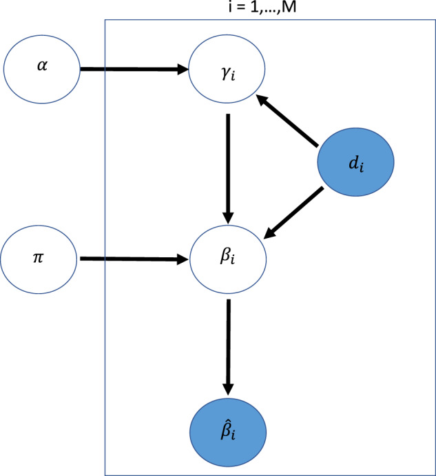
A graphical model representation of the BAGSE model. The directed acyclic graph represents a probabilistic generative model. The shaded variables represent data that are observed
With observed association data and annotation data , we frame the problem of enrichment analysis as an inference problem with respect to the enrichment parameter .
2.2 Gene set enrichment estimation
To quantify the enrichment level of annotated genes within a pre-defined gene set, we perform MLE with respect to based on the proposed hierarchical model. Particularly, we design an expectation and maximization (EM) algorithm to obtain the MLEs for hyperparameters by treating the latent binary vector as missing data.
Briefly, in the E-step of the t-th iteration we evaluate the probability for all genes (where and denote the current estimates of and , respectively). In this process, the unknown effect size parameters, βi’s, are analytically integrated out. In the M-step, we simply fit a logistic regression model
| (4) |
and use the resulting generalized linear model estimates of α0 and α1 to obtain the updated . Subsequently, is computed by maximizing a simple K-dimensional multinomial likelihood function.
We start the algorithm from a set of arbitrary values of and and iterate between the E and M steps until the pre-defined convergence criteria are met. The standard error of is computed using a profile likelihood approach. The full details of the EM algorithm are provided in the Supplementary Material. Finally, we summarize the result of the gene set enrichment analysis by constructing a 95% confidence interval (CI) of α1 from the EM output. Furthermore, we can obtain a P-value by computing a z-statistic from and its standard error to test the null hypothesis,
| (5) |
2.3 A latent contingency table interpretation
Here, we provide an intuitive and general view of our enrichment analysis model and algorithm. Without loss of generality, we consider a single binary annotation for a particular gene set definition (i.e. a gene is either in or out of the annotated pathway/gene set). Now consider an ideal (but unrealistic) scenario where the true association status of each gene is indeed known. Under this setting, the enrichment analysis can be formulated as a 2 × 2 contingency table with the four cells indicating the four possible combinations of association and annotation status. Given the table, it is straightforward to compute the odds ratio to quantify the level of enrichment. It should be known that the enrichment computation from the contingency table is also statistically equivalent to fitting a simple logistic regression model. However, in practice, the exact classification of the association status is unknown, and the above simple procedure is not directly applicable.
As mentioned in the introduction, the commonly applied two-stage procedure can be viewed as an ad-hoc procedure to fill in the unobserved 2 × 2 contingency table based on a simple classification rule. That is, a gene is classified as ‘associated’ if the null hypothesis from a statistical test is rejected, and ‘unassociated’ otherwise. This procedure is intuitive but has some notable caveats. Importantly, it should be clear that the ‘filled’ contingency table is not necessarily accurate compared to the underlying true table. This is because adopting hypothesis testing as a classification procedure preferentially restricts type I errors (false positives) but not the overall classification errors, in which type II (false negatives) errors make up a substantial proportion and are not controlled.
To demonstrate this point, we perform simulations and apply the two-stage procedure to estimate the enrichment parameter. In each simulation, we first generate a 2 × 2 contingency table given the true association and annotation status. We subsequently adjust the cell counts to reflect both the type I and type II errors in the gene-level hypothesis testing. Finally, we compute the enrichment parameter α1 using the adjusted contingency table. In summary, we find that the two-stage procedure consistently yields the enrichment estimates that are biased toward 0. With the type I error under control, the degree of bias is negatively correlated with the power of gene-level tests. An example from the simulation study is shown in Supplementary Figure S2. Interestingly, the lower power of the gene-level tests is also associated with a higher degree of variation in the enrichment estimates from the adjusted contingency table. Therefore, we conclude that the two-stage procedure can be inaccurate in estimating the enrichment parameter. Nevertheless, for enrichment testing, the direction of the bias from the two-stage procedure seems only to impact power but does not inflate the type I error that asserts enrichment when , as can be noted from results in Supplementary Table S2.
Our proposed EM algorithm, in this case, can be viewed as an iterative approach to fill in the unobserved contingency table, accounting for the uncertainty of the true binary association status. In the E-step of the proposed EM algorithm, we essentially fill in the table with the expected values of each gene. Note that
| (6) |
Hence, gene i contributes to the cell count of associated and annotated by an amount of , and to the cell count of unassociated and annotated by an amount of . An obvious advantage of this approach is that the uncertainty of the association analysis result is accounted for. The M-step is essentially the same statistical procedure given the contingency table is filled with the expected cell counts.
2.4 Local FDR control accounting for gene set enrichment
Another unique advantage of BAGSE is that the estimated enrichment information can be subsequently utilized in identifying truly associated candidate genes. Intuitively, accounting for the quantitative enrichment information boosts the power in identifying signals. This is accomplished by expanding a parametric empirical Bayes framework of local false discovery rate (FDR) control procedure described in Stephens (2017). Specifically, we consider testing the null hypothesis for all genes using the enrichment information. For each test, we evaluate the local FDR (lfdr) by plugging in the enrichment estimate ,
| (7) |
which is a byproduct of our EM algorithm and can be directly applied to control FDR.
Our proposed procedure also provides a principled solution to deal with non-exchangeable multiple hypothesis testing. For example, one may suspect that genes in certain annotated pathways are more likely to be true signals. Such prior expectations can be precisely expressed by Equation (2) in our model. In particular, if and gene i is a member of the gene set of interest, then it has a higher prior probability to be a genuine signal compared to its counterparts absent from the gene set. Furthermore, the enrichment estimation procedure outlined in the EM algorithm allows us to effectively learn the value of α1 from the observed data. The lfdr computed in (7) combines the enrichment prior and the likelihood information observed from data: if a gene set is estimated to be enriched, the lfdrs of its member genes are down-weighted by the priors.
In addition to controlling FDR for testing presence or absence of signals (i.e. γi’s), our approach can be extended to control the local false sign rates (Stephens, 2017), which focus on the signals whose effects can be identified robustly. In particular, we compute local false sign rates for gene i by
| (8) |
which is interpreted as the error probability in determining the sign of the effect for gene i.
2.5 Use of multi-category gene set annotations
A unique advantage of BAGSE for enrichment analysis is that it can easily handle multiple gene set annotations, which generalizes the commonly used binary annotations. Consider L potentially overlapping gene sets that we wish to evaluate simultaneously. A gene can be independently annotated (i.e. in or out) by an individual annotation. The joint annotation of a gene can be represented by a binary L-vector, which can take possible values: for example, indicates a gene is not annotated in any gene set, and indicates a gene is annotated in all gene sets. Note that our parametric prior model (2) can accommodate such multi-category annotation by regarding the corresponding di as a categorical variable coded by dummy variables (Supplementary Section S1.2). For inference, instead of reporting a single enrichment coefficient (α1), the use of multi-category annotation leads to up to enrichment coefficients for different annotation configurations in contrast to the baseline annotation .
The general scheme applies to an arbitrary number of gene sets (L) considered, although a large number of L values may lead to expensive computational costs. It is possible to make simplifying assumptions to reduce computational complexity. For example, let binary indicator denotes if gene i is annotated in the gene set l. We consider an additive prior model
| (9) |
which is computationally feasible for moderate to large L values. This particular prior model is also implemented in the BAGSE.
One of the unique advantages of the multi-category gene set annotation is to maximize the utility of the proposed FDR control procedure. In Gene Ontology (GO) and KEGG pathways, a single gene is often annotated in multiple gene sets. Relying on a single gene set to determine the lfdr of the given gene seems sub-optimal. The logical alternative is to combine the multiple gene sets and generate a single multi-category gene set annotation. We argue that such annotation provides objective and optimal FDR control to maximize the discovery power by incorporating information from gene set annotations. We demonstrate this point in a real data application described in Section 3.3.
3 Results
3.1 Simulation studies
We use numerical simulations to benchmark the performance of the proposed Bayesian gene set enrichment analysis procedure. Our particular focuses are put on examining the accuracy of the enrichment estimates and the performance of the proposed approach in enrichment testing.
In each simulated dataset, we consider the analysis of 10 000 genes, each of which is assigned a binary true association status based on the enrichment parameters () and pre-defined annotations. For each gene, we assume an association z-score is available for the enrichment analysis: for unassociated genes, we draw the z-scores from the standard normal distribution; for the associated genes, the z-scores are simulated from a t-distribution with the degree of freedom (which mimics the long-tailed effect size distribution commonly observed in practice, see Supplementary Fig. S1). We set the enrichment parameter throughout, while varying the values of α1 and the proportion of annotated genes (denoted by q) across all simulations. We vary α1 values from 0 to 1, due to all investigated methods having power similarly near power as α1 increases to above 1. We use values for q ranging from to , due to that being a realistic range for q based on the hierarchical nature of popular databases such as KEGG or GO. Each parameter set is used to generate 5000 different datasets.
3.1.1 Evaluation of enrichment parameter estimation
We first examine the point estimate of the enrichment parameter from the BAGSE analysis procedure. For comparison, we also compute the enrichment estimate from the two-stage procedure. The analysis results of the simulated datasets are summarized in Figure 2 for annotation proportion . It is clear that the proposed approach consistently yields unbiased enrichment estimates across all α1 values. Also consistent with the previous results, the estimates from the two-stage approach are biased toward 0. Across different q values, the estimates from the Bayesian procedure remain unbiased. But we observe a pattern that shows a lower level of variation in when q increases toward 0.5. The latent contingency table interpretation can intuitively explain this phenomenon: as q tends to 0 (or 1), the underlying table becomes more imbalanced, causing increased uncertainty for the enrichment parameter. Results from simulations using all parameter sets can be found in Supplementary Table S1 and Supplementary Figures S3–S5.
Fig. 2.
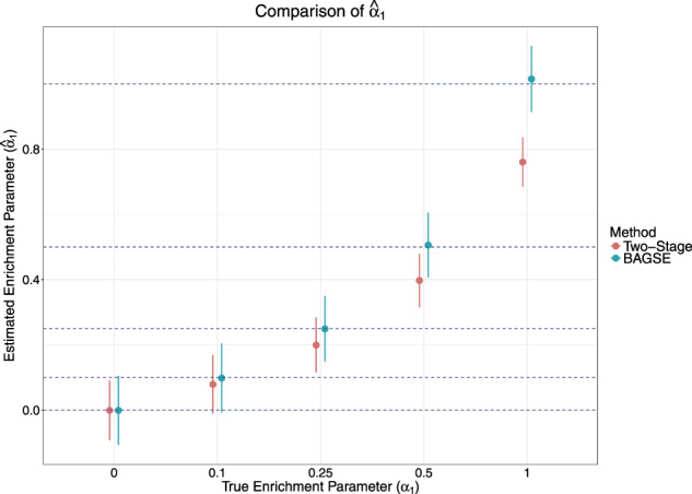
A comparison of the enrichment parameter estimates between the two-stage approach and the proposed method, with standard errors represented as error bars. BAGSE appears to give an unbiased estimate of α1, while the two-stage approach’s estimate grows more severely biased as the enrichment parameter grows higher
We conduct additional simulations to illustrate the ability of the proposed method in estimating enrichment parameters using annotations from multiple overlapping gene sets. In summary, we find that BAGSE estimates in such a scenario remain unbiased and accurate. The details of these additional simulations are described in Supplementary Section S2.
3.1.2 Power comparison in enrichment testing
Next, we proceed to examine the performance of various methods, including BAGSE, the two-stage approach, and the popular GSEA method, in testing the enrichment hypothesis: . We apply both the unweighted and weighted forms of the GSEA procedure. The unweighted GSEA procedure corresponds to a standard Kolmogorov–Smirnov test (by comparing the distribution of the absolute value of z-scores, or P-values, between annotated and unannotated genes). We use the default weight recommended in the original GSEA paper (Subramanian et al., 2005) to perform the weighted GSEA procedure.
The simulation results for when are summarized in Figure 3. We conclude that all methods properly control type I errors at 5% level, based on the proportion of tests rejected when being below 0.05 (denoted by the dotted line) for all methods. BAGSE and the weighted GSEA method are top performers at every combination of simulation parameters, constantly outperforming the unweighted GSEA and the two-stage approaches by a significant margin, especially at the intermediate α1 values of 0.1 and 0.25. The power difference between BAGSE and the weighted GSEA is generally negligible. In our simulation setting, when , all methods seemingly achieve the perfect power to reject the null hypothesis. Additionally, we observe that the power to detect enrichment improves as q increases toward 0.5. This phenomenon can be similarly explained by the latent contingency table interpretation of our proposed model: the standard error of the enrichment estimate decreases as the proportion of the annotation increase toward 0.5. Results from simulations using all parameter sets for all methods can be found in Supplementary Table S2 and Supplementary Figures S6–S8.
Fig. 3.
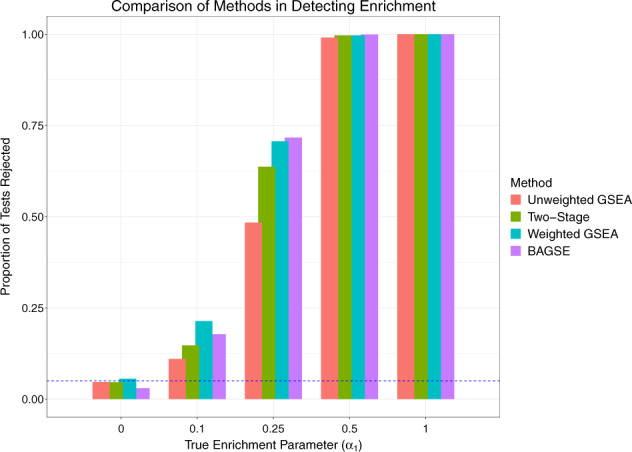
A comparison of type I error and power to detect gene set enrichment using unweighted GSEA, two-stage approach, weighted GSEA and BAGSE. The y-axis denotes the proportions of simulated datasets where the null hypothesis is rejected. The leftmost columns, corresponding to the null model , represent the type I error rates for the methods. As the enrichment parameter takes non-zero values, the data are simulated under the alternative scenarios, and the corresponding columns represent the power. All methods control the type I errors properly. As expected, power for all methods increases as the true enrichment parameter increases. BAGSE and weighted GSEA outperform the other methods in this regard
3.1.3 Gene discovery incorporating enrichment quantification
Finally, we examine the power in identifying truly associated genes when gene set enrichment information is explicitly considered. Specifically, we compute the lfdr for each gene using (7) where the estimated enrichment parameter is plugged in, and control the overall FDR at 5% level. For a baseline comparison, we use both the q-value procedure (Storey et al., 2003) and the lfdr procedure (both are implemented in the R package ‘qvalue’) to control FDR at the same level ignoring the gene set information.
Our results indicate that all methods properly control the FDR at the desired level. However, the proposed procedure accounting for enrichment quantification consistently outperforms the q-value and the lfdr procedure ignoring the enrichment information in realized power (Fig. 4). As expected, the improvement of power is positively correlated with the level of enrichment. In our simulation setting, we observe a modest increase in power (, or 20 more true positive discoveries per simulated dataset) when the enrichment parameter is ; as α1 reaches 5, the power boost becomes much more substantial ( improvement in power, or 400 more true discoveries per simulated dataset).
Fig. 4.

Power increment in gene discovery when accounting for gene set enrichment information. The percentages of power increment by using enrichment information are compared to two standard FDR control procedures: the q-value method (solid line) and the lfdr method (dashed line). All methods control FDR at 5% level
3.2 Real data application I: DE experiment
Next, we apply BAGSE to the experimental data from Moyerbrailean et al. (2016), which considers the DE of genes under the treatment of glucocorticoid. The study profiles 20 896 genes using RNA-seq. A P-value is obtained for each gene using the software package DESeq2 (Love et al., 2014). We convert the P-values into the z-scores, using the estimated effect sizes from the study to determine the corresponding signs. The experiments are also carried out in multiple tissues. For demonstration purposes, we select the results gathered from the peripheral blood mononuclear cells. Because of the known nature of these cells in their response to glucocorticoid, we expect genes involved in pathways associated with immune response to be enriched.
There are 21 KEGG pathways involved in the immune responses. Of these, 15 contain genes that are in our dataset. We first analyze these 15 pathways separately using BAGSE. The enrichment estimate for each of these pathways is provided in Supplementary Table S3. We observe that the majority of the examined pathways (12 out of 15) are shown to be significantly enriched with DE genes, and their enrichment levels can be straightforwardly compared by utilizing the quantified enrichment estimates. In particular, we find that the intestinal immune network for IgA production pathway seemingly shows an extremely high level of enrichment [ with 95% CI (5.38–13.29)].
Because each pathway only annotates a small proportion of genes, the CIs are typically large (Supplementary Table S3). Following Carbonetto and Stephens (2013), we pool the genes annotated in the 15 KEGG pathways to form a general category of the gene set and examine the enrichment of DE genes in this gene set representing general immune responses. In total, 2.7% of the 20 896 genes are annotated in the aggregated gene set.
We apply BAGSE, the two-stage approach, and GSEA with the two different weighting schemes to conduct gene set enrichment analysis. These results are summarized in Table 1. BAGSE detected strong enrichment for the pooled immune response gene sets, with an enrichment log odds ratio of 1.31 [95% CI (0.96–1.66)], which corresponds to a P-value of . The two-stage approach also detects enrichment, with an enrichment log odds ratio of 0.87 [95% CI (0.63–1.11)]. The unweighted GSEA method detects significant enrichment with a P-value of . The weighted GSEA method also detects significant enrichment with an estimated P-value .
Table 1.
The comparison of significance in detecting enrichment between methods for data from the differential expression of genes under treatment of glucocorticoid
| Method | P-value | Enrichment estimate (95% CI) |
|---|---|---|
| BAGSE | 1.31 (0.96, –1.66) | |
| Two-stage | 0.87 (0.63, –1.11) | |
| Unweighted GSEA | — | |
| Weighted GSEA | < | — |
Note: As expected, all methods show significance. Note that the inexact value for the weighted GSEA P-value is due to its calculation using 1000 permutations [recommended by Subramanian et al. (2005)].
Additionally, we examine the power improvement in identifying DE genes by incorporating the quantified enrichment information. Without using the enrichment information, we find that the q-value procedure identifies 1496 genes at 5% FDR level (the lfdr procedure, implemented in the q-value package, identifies 1527 genes). By incorporating the enrichment estimates, BAGSE identifies 1617 genes at the same FDR control level, which amounts to 8% increase in comparison to the q-value procedure (or 6% increase to the lfdr procedure). Overall, these results appear consistent with our simulation studies.
3.3 Real data application II: TWAS analysis
For the second illustration with real data, we perform gene set enrichment analysis using the association results generated from the TWAS analysis. TWAS is a principled approach based on Mendelian randomization and attempts to test potential causal relationships from the expressions of candidate genes to the complex trait of interest (Gamazon et al., 2015; Gusev et al., 2018; Zhu et al., 2016). Specifically, TWAS analysis constructs a genetic gene expression prediction function using the eQTL data and examines the association between the predicted gene expression levels and the complex trait of interest from the GWAS data.
In this example, we use the GWAS summary statistics of high-density lipoprotein levels from the Global Lipids Genetics Consortium (Willer et al., 2013) and the multi-tissue eQTL data from the GTEx project (version 8) (GTEx Consortium, 2019). We apply the S-PrediXcan (Barbeira et al., 2016) algorithm and obtain TWAS P-values for a total of 32 362 genes that are investigated in the GTEx project.
Based on the TWAS association statistics, we investigate the enrichment of six gene sets from KEGG and GO. These gene sets are implicated in the original Global Lipids Genetics Consortium analysis (Willer et al., 2013) by the MAGENTA method (Segrè et al., 2010). The original analysis uses a proximity-based approach and painstaking biological analysis to link a GWAS hit to a nearby gene (in comparison, the TWAS analysis establishes the links automatically with the aid of additional eQTL data and few subjective criteria). With the gene-level quantification directly obtained from the TWAS analysis, we aim to re-examine the results, which have been considered as a gold standard in lipids genetic research.
The results of the enrichment analysis of the six gene sets by BAGSE and weighted GSEA are summarized in Table 2. At the significance level of 0.05, BAGSE identifies enrichment in five of the six gene sets, while weighted GSEA identifies enrichment in four. We note that, in the sole gene set (triglyceride lipase activity) that barely misses the significance threshold in our BAGSE analysis, the fewest genes (15) are annotated (all remaining gene sets have at least 60 genes annotated). Consistently with what we observe in the simulation studies, precisely quantifying enrichment (i.e. with reasonably small standard errors) for such small gene sets is highly challenging. The enrichment estimates also enable direct comparison of the relative importance of these relevant biological pathways. It is not surprising that cholesterol metabolic process has the highest level of enrichment among the gene sets examined. But most importantly, this application illustrates that our proposed enrichment analysis framework has the potential to extend the causal implications derived from the TWAS analysis, and uncover the underlying causal molecular networks.
Table 2.
Summary of gene set enrichment results based on TWAS analysis of the high-density lipoprotein data from Global Lipid Genetic Consortium
| Gene sets | BAGSE enrichment estimate (95% CI) | BAGSE P-value | Weighted GSEA P-value |
|---|---|---|---|
| Neurotrophin signaling pathway (KEGG) | 1.01 (0.003, –2.03) | 0.049 | 0.052 |
| Adipocytokine signaling pathway (KEGG) | 1.24 (0.20, –2.28) | 0.019 | 0.188 |
| Triglyceride lipase activity (GO) | 1.61 (−0.008, 3.24) | 0.051 | 0.001 |
| Cholesterol metabolic process (GO) | 2.20 (1.39, –3.01) | ||
| Enzyme binding (GO) | 1.04 (0.32, –1.76) | ||
| Phospholipid binding (GO) | 1.57 (0.79, –2.35) |
Note: The TWAS analysis utilizes the multi-tissue eQTL data from the GTEx project (v8). For comparison, we also compute the enrichment testing P-values from the weighted GSEA approach. All gene sets, with the exception of the triglyceride lipase activity, show enrichment at the 5% significance level in BAGSE results. However, their point estimates and the corresponding standard errors vary. The variations of the standard errors can mainly be attributed to number of annotated genes.
Additionally, we again confirm that incorporating enrichment information helps improve the power of association discovery. In this instance, the original TWAS analysis (without enrichment information) identifies 578 unique genes at FDR 5% level. By incorporating the enrichment estimate from cholesterol metabolic process, we identify an additional 30 genes at the same FDR level, representing a 5% increase in discovery. Finally, we combine the three significant GO terms into a single multi-category gene set annotation and repeat the enrichment estimation and the FDR control procedure. In the end, we find 626 genes are rejected at the FDR 5% level, representing an 8% increase in discovery.
4 Discussion
In this paper, we have introduced an empirical Bayes procedure, denoted as BAGSE, for gene set enrichment analysis. We have shown, through simulations and real data analysis, that the proposed approach provides a principled inference procedure to estimate the level of enrichment for a gene set, avoiding the caveats of the two-stage procedure. In addition, the proposed Bayesian method maintains strong power in testing enrichment as compared to other popular approaches to gene set enrichment analysis. Finally, we show that the enrichment estimates from the proposed approach can be subsequently utilized to improve power for gene-level testing.
It should be noted that our approach can be straightforwardly applied to simultaneously estimate the enrichment of multiple gene sets with overlapping genes. This unique feature can be critical because, as seen in many commonly used gene pathway definitions (e.g. the KEGG pathway database), there are many genes involved in multiple pathways. This flexibility in gene annotation intrinsic to the proposed Bayesian model gives it a distinct advantage as an enrichment analysis method.
During our simulations, we noted that both the power to detect enrichment and enrichment estimation were heavily dependent on the proportion of genes annotated. Our latent contingency table interpretation can partially explain this phenomenon: even if all association status is indeed observed, the standard error of the enrichment estimate is known to be negatively correlated with the smallest cell count, and lower annotation proportion tends to decrease the smallest cell count (which typically is the cell corresponds to the count of both annotated and associated genes). All enrichment testing and estimation methods would be affected by a low proportion of annotated genes, reflected by losing either power or precision. In general, the quality of the gene set definition has a direct impact on results from enrichment analysis. Defining highly specific gene pathways is an ongoing challenge.
In our real data applications, we illustrate the proposed gene set enrichment analysis based on TWAS results. TWAS analysis focuses on assessing the potential causal relationship from a single gene to a complex trait of interest. The gene set enrichment analysis based on TWAS results has the potential to extend the causal implications of single genes and uncover potentially causal biological pathways. We expect that this type of analysis will become increasingly popular in the field of systems biology. Our proposed approach has the unique advantage in accurate quantification of relative enrichment levels of candidate gene sets, which should aid in comparing and selecting causal molecular pathways of complex diseases.
Funding
This work is supported by the NIH grants R01GM109215 and R01AR042742.
Conflict of Interest: none declared.
Supplementary Material
References
- Barbeira A. et al. (2016) MetaXcan: summary statistics based gene-level association method infers accurate prediXcan results. bioRxiv. 045260. doi: 10.1101/045260. [Google Scholar]
- Carbonetto P., Stephens M. (2013) Integrated enrichment analysis of variants and pathways in genome-wide association studies indicates central role for il-2 signaling genes in type 1 diabetes, and cytokine signaling genes in Crohn’s disease. PLoS Genet., 9, e1003770. [DOI] [PMC free article] [PubMed] [Google Scholar]
- Chang Y. et al. (2016) COPD subtypes identified by network-based clustering of blood gene expression. Genomics, 107, 51–58. [DOI] [PMC free article] [PubMed] [Google Scholar]
- Efron B. (2012) Large-Scale Inference: Empirical Bayes Methods for Estimation, Testing, and Prediction. Vol. 1 Cambridge University Press, Cambridge. [Google Scholar]
- Elovainio M. et al. (2015) Activated immune–inflammatory pathways are associated with long-standing depressive symptoms: evidence from gene-set enrichment analyses in the Young Finns Study. J. Psychiatr. Res., 71, 120–125. [DOI] [PubMed] [Google Scholar]
- Gamazon E.R. et al. (2015) A gene-based association method for mapping traits using reference transcriptome data. Nat. Genet., 47, 1091. [DOI] [PMC free article] [PubMed] [Google Scholar]
- GTEx Consortium (2019) The GTEx Consortium atlas of genetic regulatory effects across human tissues. bioRxiv. 787903. doi: 10.1101/787903. [DOI] [PMC free article] [PubMed] [Google Scholar]
- Gusev A. et al. (2018) Transcriptome-wide association study of schizophrenia and chromatin activity yields mechanistic disease insights. Nat. Genet., 50, 538. [DOI] [PMC free article] [PubMed] [Google Scholar]
- Guttman M. et al. (2009) Chromatin signature reveals over a thousand highly conserved large non-coding RNAs in mammals. Nature, 458, 223. [DOI] [PMC free article] [PubMed] [Google Scholar]
- Hass J. et al. (2015) Associations between DNA methylation and schizophrenia-related intermediate phenotypes a gene set enrichment analysis. Prog. Neuropsychopharmacol. Biol. Psychiatry, 59, 31–39. [DOI] [PMC free article] [PubMed] [Google Scholar]
- Keshava Prasad T. et al. (2009) Human protein reference database 2009 update. Nucleic Acids Res., 37, D767–D772. [DOI] [PMC free article] [PubMed] [Google Scholar]
- Love M.I. et al. (2014) Moderated estimation of fold change and dispersion for RNA-seq data with DESeq2. Genome Biol., 15, 550. [DOI] [PMC free article] [PubMed] [Google Scholar]
- Maruschke M. et al. (2014) Expression profiling of metastatic renal cell carcinoma using gene set enrichment analysis. Int. J. Urol., 21, 46–51. [DOI] [PubMed] [Google Scholar]
- Mootha V.K. et al. (2003) PGC-1α-responsive genes involved in oxidative phosphorylation are coordinately downregulated in human diabetes. Nat. Genet., 34, 267. [DOI] [PubMed] [Google Scholar]
- Moyerbrailean G.A. et al. (2016) High-throughput allele-specific expression across 250 environmental conditions. Genome Res., 26, 1627–1638. [DOI] [PMC free article] [PubMed] [Google Scholar]
- Richiardi J. et al. (2015) Correlated gene expression supports synchronous activity in brain networks. Science, 348, 1241–1244. [DOI] [PMC free article] [PubMed] [Google Scholar]
- Schaub F.X. et al. (2018) Pan-cancer alterations of the MYC oncogene and its proximal network across the cancer genome atlas. Cell Syst., 6, 282–300. [DOI] [PMC free article] [PubMed] [Google Scholar]
- Segrè A.V. et al. (2010) Common inherited variation in mitochondrial genes is not enriched for associations with type 2 diabetes or related glycemic traits. PLoS Genet., 6, e1001058. [DOI] [PMC free article] [PubMed] [Google Scholar]
- Shalem O. et al. (2014) Genome-scale CRISPR-Cas9 knockout screening in human cells. Science, 343, 84–87. [DOI] [PMC free article] [PubMed] [Google Scholar]
- Speliotes E.K. et al. (2010) Association analyses of 249, 796 individuals reveal 18 new loci associated with body mass index. Nat. Genet., 42, 937. [DOI] [PMC free article] [PubMed] [Google Scholar]
- Stephens M. (2017) False discovery rates: a new deal. Biostatistics, 18, 275–294. [DOI] [PMC free article] [PubMed] [Google Scholar]
- Storey J.D. et al. (2003) The positive false discovery rate: a Bayesian interpretation and the q-value. Ann. Statist., 31, 2013–2035. [Google Scholar]
- Subramanian A. et al. (2005) Gene set enrichment analysis: a knowledge-based approach for interpreting genome-wide expression profiles. Proc. Natl. Acad. Sci. USA, 102, 15545–15550. [DOI] [PMC free article] [PubMed] [Google Scholar]
- Walter N.D. et al. (2015) Transcriptional adaptation of drug-tolerant mycobacterium tuberculosis during treatment of human tuberculosis. J. Infect. Dis., 212, 990–998. [DOI] [PMC free article] [PubMed] [Google Scholar]
- Willer C.J. et al. (2013) Discovery and refinement of loci associated with lipid levels. Nat. Genet., 45, 1274. [DOI] [PMC free article] [PubMed] [Google Scholar]
- Zhu Z. et al. (2016) Integration of summary data from GWAS and eQTL studies predicts complex trait gene targets. Nat. Genet., 48, 481. [DOI] [PubMed] [Google Scholar]
Associated Data
This section collects any data citations, data availability statements, or supplementary materials included in this article.