A Krasnoselskii-Mann Algorithm with an Improved EM Preconditioner for PET Image Reconstruction

Abstract

This paper presents a preconditioned Krasnoselskii-Mann (KM) algorithm with an improved EM preconditioner (IEM-PKMA) for higher-order total variation (HOTV) regularized positron emission tomography (PET) image reconstruction. The PET reconstruction problem can be formulated as a three-term convex optimization model consisting of the Kullback–Leibler (KL) fidelity term, a nonsmooth penalty term, and a nonnegative constraint term which is also nonsmooth. We develop an efficient KM algorithm for solving this optimization problem based on a fixed-point characterization of its solution, with a preconditioner and a momentum technique for accelerating convergence. By combining the EM precondtioner, a thresholding, and a good inexpensive estimate of the solution, we propose an improved EM preconditioner that can not only accelerate convergence but also avoid the reconstructed image being “stuck at zero.” Numerical results in this paper show that the proposed IEM-PKMA outperforms existing state-of-the-art algorithms including, the optimization transfer descent algorithm and the preconditioned L-BFGS-B algorithm for the differentiable smoothed anisotropic total variation regularized model, the preconditioned alternating projection algorithm, and the alternating direction method of multipliers for the nondifferentiable HOTV regularized model. Encouraging initial experiments using clinical data are presented.

I. Introduction

POSITRON emission tomography (PET) is a well-established technique for molecular imaging, where it can produce spatial (and temporal) estimates of a particular tracer’s bio-distribution (images). These images have been instrumental in diagnosis, staging, and are rapidly extending into therapy and response assessment. As a result, improved estimates of the tracer distribution may allow physicians and scientists to more accurately interpret the implications of these bio-distributions and improve patient outcomes. However, because of important health consideration, basic physical processes and work-flow issues, the data is inherently count and resolution limited and must be reconstructed within a few minutes of acquisition. As a result, a great deal of effort has gone into improving both the speed and accuracy of the estimation of the PET tracer distributions.

At present, these efforts have evolved in a penalized likelihood (PL) model where a data fidelity term (KL-divergence for PET, e.g., Poisson data noise models) plus one or more penalty terms to regularize the estimated images are optimized to produce the most likely image given the data and penalty. Despite the introduction of penalty terms can improve the quality of reconstructed images, these penalty terms may be nondifferentiable or even nonconvex, which makes it difficult to develop efficient algorithms for solving the PL model. To address this issue, many algorithms and penalties have been proposed, but without guidance, it is difficult to know if a particular algorithm or penalty is suitable for routine imaging.

The total variation (TV) penalty (regularization) introduced by [1] has had a great deal of success in image denoising by removing unwanted noise while preserving important details such as edges, and has been used successfully in medical imaging modalities, such as CT or MR. Unfortunately, TV can introduce piecewise constant (staircase) artifacts in the smoothly varying regions of the images, which make it unsuitable for PET. However, the addition of a second-order term, which we refer to throughout this paper as a higher-order TV (HOTV) penalty [2], [3], allows the preservation of edges at known tracer boundaries (e.g. liver, bladder, heart, brain, and, in the case of dynamic imaging, at the boundaries of blood vessels), while suppressing the undesired staircase artifacts.

Classical gradient-type algorithms are unable to solve TV or HOTV regularized models due to the nondifferentiability of their objective functions. To address this while maintaining their edge-preserving properties, [4]-[7] have used smooth approximations of the absolute value function to replace the ℓ₁ regularized model with a differentiable one. Efficient algorithms, including the preconditioned conjugate-gradient algorithm (PCG) [4], the optimization transfer descent algorithm (OTDA) [6], [8] and the preconditioned limited-memory Broyden-Fletcher-Goldfarb-Shanno with boundary constraints algorithm (L-BFGS-B-PC) [7], have been proposed for solving these smooth edge-preserving regularized models. Though the smooth approximation method used here can avoid the problem of nondifferentiability, it requires a tuning parameter, which is not part of the penalty weight. If this parameter is set too large, the smooth penalty will lose its edge-preserving property, and if it is set too small, as mentioned in [8], convergence of classical gradient-type algorithms may be slow. Therefore, it is necessary to develop new efficient algorithms to directly solve nondifferentiable models.

Recently, many algorithms have been proposed for nondifferentiable regularized models, including EM-based methods [9]-[11], projected quasi-Newton methods [12]-[14], forward-backward approach [15], primal-dual methods [16]-[18], augmented Lagrangian methods [19], [20], and fixed-point proximity methods [3], [21], [22]. Among these algorithms, the alternating direction method of multipliers (ADMM) [19], [20] and preconditioned alternating projection algorithm (PAPA) [3], [21] have shown good performance for regularized emission computed tomography (ECT) image reconstruction. In particular, [21] and [3] have shown that PAPA outperforms the nested EM-TV algorithm [11], the one-step-late method with TV regularization [9], and the preconditioned primal-dual algorithm [17], [23].

The fast proximity-gradient algorithm (FPGA) [24], derived from the multi-step fixed-point proximity framework [25], was developed for general three-term optimization problems. This algorithm has some desirable properties. For example, its development was guided by constructing an averaged nonexpansive operator for fixed-point iteration that guarantees monotone convergence. That is, as the fixed-point iteration proceeds, the distance between the iterative result and the true solution is monotone decreasing. Moreover, the inner iteration, required for ADMM, is unnecessary, which results in more stable convergence. To improve the convergence speed, FPGA introduced the Nesterov momentum technique [26], [27]. However, FPGA does not provide a strategy for choosing efficient preconditioners for three-term optimization problems.

An alternative fixed-point algorithm, PAPA, introduces the EM preconditioner instead of a step-size parameter, which greatly improves its convergence. Although the use of the EM preconditioner in PAPA makes it an efficient algorithm for solving the HOTV regularized PET reconstruction model, both PAPA and the preconditioner introduce problems. In PAPA, the use of extra-gradient step (via reuse of the forward and backward projections), makes it difficult to prove the convergence of PAPA with a momentum technique. This arises because such a method may not be reformulated as a fixed-point iteration of an averaged nonexpansive operator. Another problem is that the classical EM preconditioning matrix may not be strictly positive definite. If a component of the reconstructed image becomes zero or very close to zero at an iteration step, then this component will be stuck at zero in all the remaining iterations.

Based on the construction of averaged nonexpansive operator in FPGA and the EM preconditioner, we propose an efficient preconditioned KM algorithm (PKMA) with an improved EM (IEM) preconditioner that can be easily proven convergent with a momentum technique as well as a preconditioner, and can at the same time avoid the reconstructed images being “stuck at zero.” In PKMA, we propose a simpler but more general form of momentum parameters compared to those used in the Nesterov momentum scheme. The generality of our proposed momentum parameters is demonstrated by two properties. First, our proposed momentum parameters includes the absence of momentum as a special case. Second, we prove that the Nesterov momentum parameters are asymptotically equivalent to a special case of our proposed momentum parameters. The use of the KM based momentum scheme obtains a better approximation of the solution by adding the current fixed-point update to the difference between the current fixed-point update and the update from prior iteration. We will show that, with proper selection of a factor of the difference term (momentum term), this KM based momentum scheme can ensure faster convergence toward the solution. The KM approach is a generalization of fixed-point approach, which leads to a simple convergence proof and provides insight toward choosing the algorithmic parameters.

This paper is organized in four sections and two appendices. In section II, we first describe the HOTV regularized PET image reconstruction model, then develop a preconditioned KM algorithm with an improved EM preconditioner for solving this model. A proof for convergence of PKMA is included. Section III presents simulation results for comparison of our proposed IEM-PKMA with OTDA and L-BFGS-B-PC for the differentiable smoothed anisotropic TV (SATV) regularized model, and that with PAPA and ADMM for the nondifferentiable HOTV regularized model. Initial experiments using clinical data are also presented. Section IV offers a conclusion. In the appendices, we provide technical details for development of PKMA and analysis of its convergence.

II. PET Image Reconstruction

We develop in this section a preconditioned KM algorithm with an improved EM preconditioner for solving the HOTV regularized PET reconstruction model. Here we limit the discussion to only the case of the first-order plus the second-order TV penalty.

A. HOTV Regularized PET Image Reconstruction Model

We begin with describing the HOTV regularized PET reconstruction model. We denote by ${\mathbb{R}}_{+}$ the set of all nonnegative real numbers. For two positive integers m and d, $\mathit{A}\in {\mathbb{R}}_{+}^{m\times d}$ denotes the PET system matrix whose (i, j)^th entry equals to the probability of detection of the photon pairs emitted from the jth voxel of the radiotracer distribution $\mathit{f}\in {\mathbb{R}}_{+}^d$ within a patient (or a phantom) by the ith detector bin pair. The vector $\gamma \in {\mathbb{R}}_{+}^m$ represents the mean value of the background noise from random and scatter coincidences. The relation of projection data $\mathit{g}\in {\mathbb{R}}_{+}^m$ of a PET system with the radiotracer distribution f can be described by the Poisson model

$$\mathit{g}=\text{Poisson}(\mathit{A}\mathit{f}+\gamma ),$$ (1)

where Poisson(x) denotes a Poisson-distributed random vector with mean x. System (1) may be solved by minimizing the following fidelity term

$$F(\mathit{f})≔\langle \mathit{A}\mathit{f},1_m\rangle -\langle \text{ln}(\mathit{A}\mathit{f}+\gamma ),\mathit{g}\rangle ,$$ (2)

where $1_m\in {\mathbb{R}}^m$ is the vector whose components are all 1, the logarithmic function at $\mathit{x}\in {\mathbb{R}}^n$ is defined by ln x := [ln x₁, ln x₂, … , ln x_n]^⊤, and $\langle \mathit{x},\mathit{y}\rangle ≔{\sum }_{i=1}^n{x}_i{y}_i$ is the inner product of x, $\mathit{y}\in {\mathbb{R}}^n$.

Minimization of the fidelity term is well-known to be ill-posed [5], which results in severe over-fitting in the reconstructed image. To avoid this over-fitting problem, regularization terms were introduced as part of the reconstruction model. In this study, using both the first-order and the second-order TV penalties, we get the following HOTV regularized PET image reconstruction model

$$\underset{f\in {\mathbb{R}}^d}{\text{arg min}}\{F(\mathit{f})+{\lambda }_1({\phi }_1\circ {\mathit{B}}_1)(\mathit{f})+{\lambda }_2({\phi }_2\circ {\mathit{B}}_2)(\mathit{f})+ı(\mathit{f})\},$$ (3)

where φ₁ ∘ B₁ and φ₂ ∘ B₂ represent the first-order and second-order TV, respectively. The two functions φ₁, φ₂ are defined by the ℓ₁-norm for the anisotropic TV or the ℓ₂-norm for the isotropic TV, and thus they are convex. Here ${\mathit{B}}_1\in {\mathbb{R}}^{m_1\times d}$, ${\mathit{B}}_2\in {\mathbb{R}}^{m_2\times d}$ are the first-order and second-order difference matrices, respectively, and λ₁, ${\lambda }_2\in {\mathbb{R}}_{+}$ are the corresponding regularization parameters. For the detailed definitions of φ₁, φ₂ and B₁, B₂, see Appendix A. The indicator function ı on ${\mathbb{R}}_{+}^d$ is defined by

$$ı(\mathit{x})≔\{\begin{array}{cc}0,\hfill & \text{if}\mathit{x}\in {\mathbb{R}}_{+}^d,\hfill \\ +\infty ,\hfill & \text{else}.\hfill \end{array}\phantom{\}}$$

To simplify notation, we define m₀ := m₁ + m₂, for $z≔\left[\begin{array}{c}\hfill \mathit{x}\hfill \\ \hfill \mathit{y}\hfill \end{array}\right]\in {\mathbb{R}}^{m_0}$ with $\mathit{x}\in {\mathbb{R}}^{m_1}$, $\mathit{y}\in {\mathbb{R}}^{m_2}$,

$$\phi (z)≔{\lambda }_1{\phi }_1(\mathit{x})+{\lambda }_2{\phi }_2(y),\text{and}\mathit{B}≔\left[\begin{array}{c}\hfill {\mathit{B}}_1\hfill \\ \hfill {\mathit{B}}_2\hfill \end{array}\right].$$ (4)

Then model (3) can be written in a compact form

$$\underset{f\in {\mathbb{R}}^d}{\text{arg min}}\{F(\mathit{f})+\phi (\mathit{B}\mathit{f})+ı(\mathit{f})\}.$$ (5)

This is the model on which the proposed reconstruction algorithm is based.

B. Preconditioned Krasnoselskii-Mann Algorithm

We next characterize a solution of model (5) as a fixed-point of a mapping defined via the proximity operator of functions φ and ı. To this end, we let ${\mathbb{S}}_{+}^n$ denote the set of n × n symmetric positive definite matrices. For $\mathit{H}\in {\mathbb{S}}_{+}^n$, the H-weighted inner product is defined by ⟨x, y⟩_H := ⟨x, Hy⟩ for x, $\mathit{y}\in {\mathbb{R}}^n$ and the corresponding H-weighted ℓ₂-norm is defined by $\Vert \mathit{x}{\Vert }_{\mathit{H}}≔\langle \mathit{x},\mathit{x}{{\rangle }_{\mathit{H}}}^{\frac{1}{2}}$. According to [28], for a convex function $\psi :{\mathbb{R}}^n\to \mathbb{R}$, the proximity operator of ψ with respect to $\mathit{H}\in {\mathbb{S}}_{+}^n$ at $\mathit{x}\in {\mathbb{R}}^n$ is defined by

$${\text{prox}}_{\psi ,\mathit{H}}(\mathit{x})≔\underset{u\in {\mathbb{R}}^n}{\text{arg min}}\left\{\frac{1}{2}\Vert \mathit{u}-\mathit{x}{\Vert }_{\mathit{H}}^2+\psi (\mathit{u})\right\}.$$

In particular, we use prox_ψ for prox_ψ,I. We let ${\Gamma }_0({\mathbb{R}}^n)$ denote the class of all proper lower semicontinuous convex functions defined on ${\mathbb{R}}^n$ and recall that the conjugate ψ* of ψ is defined by ${\psi }^{\ast }(z)≔{\text{sup}}_{\mathit{x}\in {\mathbb{R}}^n}\{\langle \mathit{z},\mathit{x}\rangle -\psi (\mathit{x})\}$. Now we have the following fixed-point characterization of a solution of model (5).

Theorem 1: If $\mathit{f}\in {\mathbb{R}}^d$ is a solution of model (5), then for any $\mathit{P}\in {\mathbb{S}}_{+}^d$ and $\mathit{Q}\in {\mathbb{S}}_{+}^{m_0}$, there exists a vector $\mathit{h}\in {\mathbb{R}}^{m_0}$ such that

$$\mathit{f}={\text{prox}}_{ı,{\mathit{P}}^{-1}}\left(\mathit{f}-\mathit{P}(\nabla F(\mathit{f})+{\mathit{B}}^{\mathsf{T}}\mathit{h})\right),$$ (6)

$$\mathit{h}={\text{prox}}_{{\phi }^{\ast },{\mathit{Q}}^{-1}}(\mathit{h}+\mathit{Q}\mathit{B}\mathit{f}).$$ (7)

Conversely, if there exist $\mathit{P}\in {\mathbb{S}}_{+}^d$, $\mathit{Q}\in {\mathbb{S}}_{+}^{m_0}$, and $\mathit{h}\in {\mathbb{R}}^{m_0}$ such that $\mathit{f}\in {\mathbb{R}}^d$ satisfies equations (6) and (7), then f is a solution of model (5).

Proof: It can be verified that in (5), $F:{\mathbb{R}}^d\to \mathbb{R}$ is convex and differentiable with a Lipschitz continuous gradient, $\phi \in {\Gamma }_0({\mathbb{R}}^{m_0})$ and $ı\in {\Gamma }_0({\mathbb{R}}^d)$. Using [21, Th. 3.1], we conclude that this theorem holds true. ■

Note that the gradient of the fidelity term F is given by

$$\nabla F(\mathit{f})={\mathit{A}}^{\mathsf{T}}\left(1_m-\frac{\mathit{g}}{\mathit{A}\mathit{f}+\gamma }\right).$$ (8)

We shall develop a convergent efficient algorithm for solving model (5) from the fixed-point equations (6) and (7). To this end, we write equations (6) and (7) in a compact form. Define

$$\mathit{v}≔\left[\begin{array}{c}\hfill \mathit{f}\hfill \\ \hfill \mathit{h}\hfill \end{array}\right]\in {\mathbb{R}}^{d+m_0},r(\mathit{v})≔F(\mathit{f}),$$ (9)

$$T(\mathit{v})≔\left[\begin{array}{c}\hfill {\text{prox}}_{ı,{\mathit{P}}^{-1}}(\mathit{f})\hfill \\ \hfill {\text{prox}}_{{\phi }^{\ast },{\mathit{Q}}^{-1}}(\mathit{h})\hfill \end{array}\right],\mathit{E}≔\left[\begin{array}{cc}\hfill {\mathit{I}}_d\hfill & \hfill -{\mathit{PB}}^{\mathsf{T}}\hfill \\ \hfill \mathit{QB}\hfill & \hfill {\mathit{I}}_{m_0}\hfill \end{array}\right],$$

where I_n denotes the n × n identity matrix, $\mathit{P}\in {\mathbb{S}}_{+}^d$, $\mathit{Q}\in {\mathbb{S}}_{+}^{m_0}$ are two introduced preconditioning matrices, and define

$$\mathit{R}≔\left[\begin{array}{cc}\hfill \mathit{P}\hfill & \hfill 0\hfill \\ \hfill 0\hfill & \hfill \mathit{Q}\hfill \end{array}\right].$$ (10)

For the matrix $\mathit{E}\in {\mathbb{R}}^{(d+m_0)\times (d+m_0)}$ and the operator $\mathit{R}\nabla r:{\mathbb{R}}^{d+m_0}\to {\mathbb{R}}^{d+m_0}$, we define E – R∇r by (E – R∇r)(v) := E(v)–R∇r(v) for $\mathit{v}\in {\mathbb{R}}^{d+m_0}$. Then (6) and (7) can be written as the fixed-point equation of T composed with E – R∇r,

$$\mathit{v}=(T\circ (\mathit{E}-\mathit{R}\nabla r))(\mathit{v}).$$

This means that if v := [v₁, v₂, …, v_d+m0]^⊤ is a fixed-point of T ∘ (E – R∇r), then f = [v₁, v₂, … , v_d]^⊤, the subvector of the first d components of v, is a solution of model (5). It was shown in [25] that E is expansive. The fixed-point iteration of T ∘ (E – R∇r) may fail to yield a convergent sequence. To develop a convergent fixed-point algorithm, we choose matrix $\mathit{G}\in {\mathbb{R}}^{(d+m_0)\times (d+m_0)}$ by

$$\mathit{G}≔\left[\begin{array}{cc}\hfill {\mathit{I}}_d\hfill & \hfill -{\mathit{PB}}^{\mathsf{T}}\hfill \\ \hfill -\mathit{QB}\hfill & \hfill {\mathit{I}}_{m_0}\hfill \end{array}\right]$$ (11)

and proceed the fixed-point iteration

$${\mathit{v}}^{k+1}=T\left((\mathit{E}-\mathit{G}){\mathit{v}}^{k+1}+(\mathit{G}-\mathit{R}\nabla r){\mathit{v}}^k\right),k\in {\mathbb{N}}_0,$$ (12)

where ${\mathbb{N}}_0≔\{0,1,\dots \}$. The iteration (12) is in fact explicit since E – G is strictly block lower triangular (in the block partition as E). We define $T_{\mathit{G}}:{\mathbb{R}}^{d+m_0}\to {\mathbb{R}}^{d+m_0}$ by

$$T_{\mathit{G}}:\mathit{u}\to \left\{\begin{array}{c}\hfill \mathit{v}:(\mathit{u},\mathit{v})\text{satisfies that}\hfill \\ \hfill \mathit{v}=T((\mathit{E}-\mathit{G})\mathit{v}+\mathit{Gv})\hfill \end{array}\right\},$$ (13)

W := R⁻¹G, and let

$${\mathcal{T}}_W:=T_G\circ (\mathcal{I}-W^{-1}\nabla r),$$ (14)

where $\mathcal{I}$ denotes the identity operator.

It is important to verify that T_G is well-defined. To show this, we let $\mathit{u}≔\left[\begin{array}{c}\hfill {\tilde{\mathit{u}}}_1\hfill \\ \hfill {\tilde{\mathit{u}}}_2\hfill \end{array}\right]$ be a given vector, where ${\tilde{\mathit{u}}}_1\in {\mathbb{R}}^d$ and ${\tilde{\mathit{u}}}_2\in {\mathbb{R}}^{m_0}$. The implicit fixed-point equation (13) then can be written by

$${\tilde{\mathit{v}}}_1={\text{prox}}_{ı,{\mathit{P}}^{-1}}({\tilde{\mathit{u}}}_1-{\mathit{PB}}^{\mathsf{T}}{\tilde{\mathit{u}}}_2),$$ (15)

$${\tilde{\mathit{v}}}_2={\text{prox}}_{{\phi }^{\ast },{\mathit{Q}}^{-1}}(2\mathit{QB}{\tilde{\mathit{v}}}_1-\mathit{QB}{\tilde{\mathit{u}}}_1+{\tilde{\mathit{u}}}_2).$$ (16)

Here ${\tilde{\mathit{v}}}_1≔[v_1,v_2,\dots ,v_d{]}^{\mathsf{T}}$, ${\tilde{\mathit{v}}}_2≔[v_{d+1},v_{d+2},\dots ,v_{d+m_0}{]}^{\mathsf{T}}$. Since ${\tilde{\mathit{u}}}_1$ and ${\tilde{\mathit{u}}}_2$ in equation (15) are given, from the definition of proximity operator, we know that the solution ${\tilde{\mathit{v}}}_1$ of (15) exists and is unique, which implies the existence and uniqueness of the solution ${\tilde{\mathit{v}}}_2$ of equation (16). This shows that for any given $\mathit{u}\in {\mathbb{R}}^{d+m_0}$ in the equation contained in (13), there exists a unique solution v.

Using the definition of ${\mathcal{T}}_W$, iteration (12) can be rewritten as the fixed-point iteration

$${\mathit{v}}^{k+1}={\mathcal{T}}_W({\mathit{v}}^k),k\in {\mathbb{N}}_0.$$ (17)

We now comment on convergence of iteration (17). According to [21], ∇F is Lipschitz continuous if all components of γ are positive. Let L denote the Lipschitz constant of ∇F and λ_W the smallest eigenvalue of W. We will recall the definition of nonexpansive, firmly nonexpansive and averaged nonexpansive operators in Appendix B, and show in Lemma 7 that if ${\lambda }_W>\frac{L}{2}$, then ${\mathcal{T}}_W$ is ζ-averaged nonexpansive with respect to W, where $\zeta ≔\frac{2{\lambda }_W}{4{\lambda }_W-L}\in (\frac{1}{2},1)$. The KM theorem (Theorem 4 in Appendix B) implies that iteration (17) converges to a fixed-point of ${\mathcal{T}}_W$.

To accelerate the convergence speed of iteration (17), for α > 0, we define ${\mathcal{T}}^{\alpha }≔(1-\alpha )\mathcal{I}+\alpha {\mathcal{T}}_W$. Since ${\mathcal{T}}^{\alpha }$ is αζ-averaged nonexpansive with respect to W, by the KM theorem, we know that the fixed-point iteration

$${\mathit{v}}^{k+1}={\mathcal{T}}^{\alpha }({\mathit{v}}^k),k\in {\mathbb{N}}_0$$ (18)

converges to a fixed-point of ${\mathcal{T}}_W$ if $\alpha \in (0,\frac{1}{\zeta })$. We observe numerically that corresponding to a larger $\alpha \in (0,\frac{1}{\zeta })\subset (0,2)$, the fixed-point iteration (18) converges faster. This observation inspires us to choose α ∈ (1, 2) for (18). Iteration scheme (18) may be interpreted as an application of the momentum technique. To see this, we write

$${\mathcal{T}}^{\alpha }({\mathit{v}}^k)={\mathcal{T}}_W({\mathit{v}}^k)+(\alpha -1)({\mathcal{T}}_W({\mathit{v}}^k)-{\mathit{v}}^k),k\in {\mathbb{N}}_0.$$

Clearly, ${\mathcal{T}}^{\alpha }$ is an extension of ${\mathcal{T}}_W$ by using a momentum technique. However, we found that iteration (18) is not robust for large α ∈ (1, 2). If the components of the initial vector v⁰ are too large, to guarantee convergence, the entries of the preconditioning matrix P should be set small, which leads to slow convergence. To overcome this obstacle and obtain a robust fixed-point iteration with momentum acceleration, we use the KM iteration by allowing the momentum parameter α to vary in each iteration. That is, we introduce a sequence of parameters, for given ϱ ∈ (−1, 1) and δ ≥ 0, by

$${\alpha }_k≔1+\frac{\varrho k}{k+\delta },k\in {\mathbb{N}}_0,$$ (19)

and construct a sequence of operators

$${\mathcal{T}}^{{\alpha }_k}≔(1+{\alpha }_k)\mathcal{I}+{\alpha }_k{\mathcal{T}}_W,k\in {\mathbb{N}}_0.$$ (20)

Given an initialization ${\mathit{v}}^{(0)}\in {\mathbb{R}}^{d+m_0}$, we then proceed the KM based momentum scheme by

$${\mathit{v}}^{k+1}={\mathcal{T}}^{{\alpha }_k}({\mathit{v}}^k),k\in {\mathbb{N}}_0.$$ (21)

We next show that the Nesterov momentum parameters are asymptotically equivalent to a special case of our proposed momentum parameters, defined by (19), by appropriately setting the sub-parameters ϱ and δ. Recall that the Nesterov momentum parameters are given by

$$t_0≔1,t_{k+1}≔\frac{1+\sqrt{1+4t_k^2}}{2},{\alpha }_k^{\prime }≔1+\frac{t_k-1}{t_{k+1}},k\in {\mathbb{N}}_0.$$ (22)

When k is sufficient large, $\{{\alpha }_k^{\prime }{\}}_{k\in {\mathbb{N}}_0}$ in (22) then corresponds to $\{{\alpha }_k{\}}_{k\in {\mathbb{N}}_0}$ in (19) with the sub-parameter choice ϱ = 1 and δ = 3, in the sense given by Proposition 2. Moreover, the absence of momentum (α_k = 1 for all $k\in {\mathbb{N}}_0$) is a special case of our proposed momentum scheme with ϱ = 0, which is not the case for the Nesterov momentum since ${\alpha }_k^{\prime }>1$ for k ≥ 1. The generality of our proposed momentum scheme provides us a variety of different parameter choices for different scenarios. We now state Proposition 2, whose proof is provided in the supplementary materials. The supplementary materials are available in the supplementary files tab.

Proposition 2: Let $\{{\alpha }_k{\}}_{k\in {\mathbb{N}}_0}$ be given by (19) with ρ = 1 and δ = 3, $\{t_k{\}}_{k\in {\mathbb{N}}_0}$ and $\{{\alpha }_k^{\prime }{\}}_{k\in {\mathbb{N}}_0}$ be given by (22). Then $\{{\alpha }_k{\}}_{k\in {\mathbb{N}}_0}$ and $\{{\alpha }_k^{\prime }{\}}_{k\in {\mathbb{N}}_0}$ converge to the same value with the same convergence rate.

We now provide specific choice of preconditioning matrices P and Q for iteration (21). We let P := βS and Q := diag (ρ₁1_m1, ρ₂1_m2), where β, ρ₁ and ρ₂ are positive numbers, S is a d × d diagonal matrix with positive diagonal entries. In this case, it follows from the definition of proximity operator that for $\mathit{x}\in {\mathbb{R}}^d$,

$${\text{prox}}_{ı,{\mathit{P}}^{-1}}(\mathit{x})={\text{prox}}_{ı}(\mathit{x})={\mathit{P}}_{{\mathbb{R}}_{+}^d}(\mathit{x})≔\max (\mathit{x},0).$$ (23)

The maxima in the above equation is taken component-wise. By using the well-known Moreau decomposition [29]

$$\mathcal{I}={\text{prox}}_{{\phi }^{\ast },{\mathit{Q}}^{-1}}+\mathit{Q}\circ {\text{prox}}_{\phi ,\mathit{Q}}\circ {\mathit{Q}}^{-1},$$

and the equation

$${\text{prox}}_{\phi ,\mathit{Q}}(\mathbf{z})=\left[\begin{array}{c}\hfill {\text{prox}}_{\frac{\lambda }{{\rho }_1}{\phi }_1}(\mathit{x})\hfill \\ \hfill {\text{prox}}_{\frac{\lambda }{{\rho }_2}{\phi }_2}(\mathit{y})\hfill \end{array}\right]$$

for $\mathbf{z}:=\left[\begin{array}{c}\hfill \mathit{x}\hfill \\ \hfill \mathit{y}\hfill \end{array}\right]\in {\mathbb{R}}^{m_0}$ with $\mathit{x}\in {\mathbb{R}}^{m_1}$, $\mathit{y}\in {\mathbb{R}}^{m_2}$, we have

$${\text{prox}}_{{\phi }^{\ast },{\mathit{Q}}^{-1}}(\mathbf{z})=\left[\begin{array}{c}\hfill {\rho }_1(\mathcal{I}-{\text{prox}}_{\frac{\lambda }{{\rho }_1}{\phi }_1})(\frac{1}{{\rho }_1}\mathit{x})\hfill \\ \hfill {\rho }_2(\mathcal{I}-{\text{prox}}_{\frac{\lambda }{{\rho }_2}{\phi }_2})(\frac{1}{{\rho }_2}\mathit{y})\hfill \end{array}\right].$$

Now the preconditioned KM algorithm (PKMA) for solving model (3) is given as follows.

$$\begin{gathered} {\tilde{\mathit{f}}}^k={\mathit{P}}_{{\mathbb{R}}_{+}^d}\left({\mathit{f}}^k-\beta \mathit{S}(\nabla F({\mathit{f}}^k)+{\mathit{B}}_1^{\mathsf{T}}{\mathit{b}}^k+{\mathit{B}}_2^{\mathsf{T}}{\mathit{c}}^k)\right) \\ {\tilde{\mathit{b}}}^{k+1}={\rho }_1\left(\mathcal{I}-{\text{prox}}_{\frac{{\lambda }_1}{{\rho }_1}{\phi }_1}\right)\left(\frac{1}{{\rho }_1}{\mathit{b}}^k+{\mathit{B}}_1(2{\tilde{\mathit{f}}}^{k+1}-{\mathit{f}}^k)\right) \\ {\tilde{\mathit{c}}}^{k+1}={\rho }_2\left(\mathcal{I}-{\text{prox}}_{\frac{{\lambda }_2}{{\rho }_2}{\phi }_2}\right)\left(\frac{1}{{\rho }_2}{\mathit{c}}^k+{\mathit{B}}_2(2{\tilde{\mathit{f}}}^{k+1}-{\mathit{f}}^k)\right) \\ {\alpha }_k=1+\frac{\varrho k}{k+\delta } \\ {\mathit{f}}^{k+1}=(1-{\alpha }_k){\mathit{f}}^k+{\alpha }_k{\tilde{\mathit{f}}}^{k+1} \\ {b}^{k+1}=(1-{\alpha }_k){\mathit{b}}^k+{\alpha }_k{\tilde{\mathit{b}}}^{k+1} \\ {\mathit{c}}^{k+1}=(1-{\alpha }_k){\mathit{c}}^k+{\alpha }_k{\tilde{\mathit{c}}}^{k+1} \end{gathered}$$

One can find the explicit form of prox_ωφ1 (x) for $\mathit{x}\in {\mathbb{R}}^{m_1}$ and prox_ωφ2 (x) for $\mathit{x}\in {\mathbb{R}}^{m_2}$, where ω > 0, in Appendix A.

In the following theorem, we consider the convergence of PKMA. We let S_max denote the largest diagonal entry of the diagonal matrix S, $p≔\frac{1}{\beta {\mathit{S}}_{\max }}$ and $\xi ≔\frac{L}{2(1-\max \{\varrho ,0\})}$.

Theorem 3: Let ${\mathit{f}}^0\in {\mathbb{R}}^d$, ${\mathit{B}}^0\in {\mathbb{R}}^{m_1}$ and ${\mathit{c}}^0\in {\mathbb{R}}^{m_2}$ be given vectors, $\{{\mathit{f}}^k{\}}_{k\in {\mathbb{N}}_0}$ be the sequence generated by PKMA, where ϱ ∈ (−1, 1), δ ≥ 0 and β, ρ₁, ρ₂ are positive in PKMA. For a given diagonal matrix $\mathit{S}\in {\mathbb{R}}^{d\times d}$ with positive diagonal entries, if $\beta <\frac{1}{\xi S_{max}}$, ${\rho }_1<\frac{p-\xi }{2\Vert {\mathit{B}}_1{\Vert }_2^2+(p-\xi )\xi }$ and ${\rho }_2<\frac{p-\xi }{2\Vert {\mathit{B}}_2{\Vert }_2^2+(p-\xi )\xi }$, then $\{{\mathit{f}}^k{\}}_{k\in {\mathbb{N}}_0}$ converges to a solution of model (3).

Proof: By Theorem 8, to prove the theorem, it suffices to verify that λ_W > ξ. This is done in Lemma 9. ■

Note that in our proof, the preconditioner should be fixed in each iteration. However, we can update it during early iterations and fix it in later iterations to guarantee the convergence.

C. Improved EM Preconditioner

In this subsection, we propose an improved EM (IEM) preconditioner for PKMA to accelerate convergence. We begin by recalling the classical EM preconditioner. To avoid zero components in A^⊤1_m, we define $\Lambda \in {\mathbb{R}}^d$ as a vector such that

$${\Lambda }_j=\{\begin{array}{cc}({\mathit{A}}^{\mathsf{T}}{1}_m{)}_j,\hfill & \text{if}({\mathit{A}}^{\mathsf{T}}{1}_m{)}_j>0,\hfill \\ 1,\hfill & \text{otherwise},\hfill \end{array}\phantom{\}}$$ (24)

for j = 1, 2, …, d. As shown in [21], the EM preconditioner

$${\mathit{S}}_{\text{EM}}≔\text{diag}\left(\frac{{\mathit{f}}^k}{\Lambda }\right)$$ (25)

performs better than the identity preconditioner I_d and the diagonal normalization (DN) preconditioner

$${\mathit{S}}_{\text{DN}}≔\text{diag}\left(\frac{1_d}{\Lambda }\right).$$ (26)

However, when using the EM preconditioner, once some components of f^k are equal to zero, these components will be stuck at zero thereafter, which results in holes in the reconstructed images. Low count data and ordered subsets type algorithms, are particularly susceptible to this problem. From Theorem 3, we know that to guarantee convergence of PKMA, the entries of the diagonal preconditioning matrix S should be positive. However, this may not be the case with the EM preconditioner since some components of f^k may be zero. To guarantee the positivity of the preconditioner as well as accelerate convergence, we propose the following IEM preconditioner by including a true mean count (TMC) based thresholding and a good estimate $\widehat{\mathit{f}}$ of the true solution f* in the EM preconditioner,

$${\mathit{S}}_{\text{IEM}}(\widehat{\mathit{f}})≔\text{diag}\left(\frac{\max \{\eta 1_d,\widehat{\mathit{f}},{\mathit{f}}^k\}}{\Lambda }\right),$$ (27)

where the positive constant η is set to 0.1 · TMC and

$$\text{TMC}≔\frac{\text{ACTc}}{\text{NPFOV}\cdot \text{NPA}}.$$ (28)

Here ACTc, NPFOV, and NPA represent the total attenuation corrected true counts, the number of pixels within the field of view, and the number of projection angles, respectively.

In the definition of IEM preconditioner given by (27), our choice of the threshold constant 0.1 · TMC was based on TMC being the mean of the components of f*. In addition, as shown in Fig. 2, we empirically found that the inclusion of a good estimate of f* used in the preconditioner leads to faster convergence. This can be exploited by using a good inexpensive estimate of f* for $\widehat{\mathit{f}}$ in (27). For example, we can use an image reconstructed by filtered backprojection f_FBP as $\widehat{\mathit{f}}$. Alternatively, if we set $\widehat{\mathit{f}}=0$ in (27), then the IEM preconditioner reduces to the case considered in [30].

Fig. 2.

NOFV (left) and NRMSE (right) versus CPU time by PKMA with preconditioners S_EM, S_IEM(0), ${\mathcal{S}}_{\mathsf{IEM}}({\overline{f}}^{{}^2})$, ${\mathcal{S}}_{\mathsf{IEM}}({\overline{f}}^{{}^{20}})$ and ${\mathcal{S}}_{\mathsf{IEM}}({\overline{f}}^{{}^{200}})$.

III. Numerical Results

In this section, we present several numerical results. First, we show the performance of different choices of $\widehat{\mathit{f}}$ in the IEM preconditioner (27). Then, we compare the performance of different preconditioners and different momentum parameters for PKMA. To see the performance of PKMA with the IEM preconditioner (IEM-PKMA) for differentiable regularized PET image reconstruction model, we compare it with the existing OTDA and L-BFGS-B-PC for the SATV regularized reconstruction model. Following this, we present comparison of PKMA with two existing algorithms, PAPA and ADMM, suitable for nonsmooth penalties. Finally, we provide some initial 3D clinical results of a relaxed ordered subsets version of PKMA (ROS-PKMA).

A. Simulation Setup

We implemented the algorithms via Matlab through a 2D PET simulation model as described in [31]. The number of counts used in these 2D simulations were set to be equivalent to those from a 3D PET brain patient acquisition (administered 370 MBq FDG and imaged 1-hour post injection) collected from the central axial slice via GE D690/710 PET/CT. The resulting reference count distribution was used as the Poisson parameters for the noise realizations. An area integral projection method was used to build the projection matrix based on a cylindrical detector ring consisting of 576 detectors whose width are 4 mm. We set the FOV as 300 mm and use 288 projection angles to reconstruct a 256×256 image.

To simulate the physical factors that will affect the resolution of the reconstructed image, such as positron range, detector width, penetration, residual momentum of the positron and imperfect decoding, the phantom was convolved with an idealized (space-invariant, Gaussian) point spread function (PSF), which was set as a constant over the whole FOV. The full width half maximum (FWHM) of this PSF was set to 6.59 mm based on physical measurements from acceptance testing and [32]. The true count projection data was produced by forward-projecting the phantom convolved by the PSF. Uniform water attenuation (with the attenuation coefficient 0.096 cm⁻¹) was simulated using the PET image support. The background noise was implemented as describe in [33] and was based on 25% scatter fraction and 25% random fraction, given by SF := Sc/(Tc + Sc) and RF:=Rc/(Tc+Sc+Rc), respectively, where Tc, Sc and Rc represent true, random, and scatter counts respectively. Scatter was added by forward-projecting a highly smoothed version of the images, which was added to the attenuated image sinogram scaled by the scatter fraction. Random counts were simulated by adding a uniform distribution to the true and scatter count distributions scaled by the random fraction. We call the summation of Tc, Sc, and Rc the total counts and denote it by TC. In our simulations, we set TC = 6.8 × 10⁶ for the high-count data, and TC = 6.8 × 10⁵ for the low-count data.

We next provide the figure-of-merits used for the comparisons. They include the normalized objective function value (NOFV), normalized root mean square error (NRMSE), normalized relative contrast (NRC) and central line profile (CLP). The NOFV is defined by

$$\text{NOFV}({\mathit{f}}^k)≔\frac{\Phi ({\mathit{f}}^k)-{\Phi }_{\text{ref}}}{{\Phi }_0-{\Phi }_{\text{ref}}},$$

where Φ denotes the objective function, Φ₀ is the objective function value of the initial image, and Φ_ref denotes the reference objective function value. For simulation results, we set Φ_ref to the objective function value of the image reconstructed by 1000 iterations of IEM-PKMA. The NRMSE is defined by

$$\text{NRMSE}({\mathit{f}}^k)≔\frac{\Vert {\mathit{f}}^k-{\mathit{f}}_{\text{true}}{\Vert }_2}{\Vert {\mathit{f}}_{\text{true}}{\Vert }_2},$$

where ${\mathit{f}}_{\text{true}}\in {\mathbb{R}}^d$ is the ground truth, and ∥ · ∥₂ is the ℓ₂-norm defined by $\Vert \mathit{x}{\Vert }_2≔{\left({\sum }_{i=1}^d{x}_i^2\right)}^{\frac{1}{2}}$ for $\mathit{x}\in {\mathbb{R}}^d$. For the definition of NRC, we let ROI_H be a region within a specific hot sphere, ROI_B be a background region that is not close to any hot sphere and its size is the same as ROI_H. Define the relative contrast (RC) by $\text{RC}≔\frac{\mid E_{{\text{ROI}}_H}-E_{{\text{ROI}}_B}\mid }{E_{{\text{ROI}}_B}}$, where E_ROIH and E_ROIB represent the average activities of ROI_H and ROI_B, respectively. Then the normalized relative contrast is defined by

$$\text{NRC}({\mathit{f}}^k)≔\frac{{\text{RC}}_{{\mathit{f}}^k}}{{\text{RC}}_{\text{true}}},$$

where RC_f^k and RC_true are the relative contrast of f^k and the ground truth respectively.

Two 256 × 256 numerical phantoms shown in Fig. 1 were used for our simulations. The brain phantom was obtained from a high quality clinical PET brain image. The uniform phantom consists of the uniform background with six uniform hot spheres with distinct radii 4, 6, 8, 10, 12, 14 pixels. The activity ratio of the uniform hot spheres to the uniform background is 4:1. In the simulation experiments, we show comparison of NOFV, NRMSE by reconstructing the brain phantom, and NRC, CLP by reconstructing the uniform phantom. All simulations were performed in a 64-bit windows 10 laptop with Intel Core i7-7500U Processor at 2.70 GHz, 8 GB of DDR4 memory and 256GB SATA SSD.

Fig. 1.

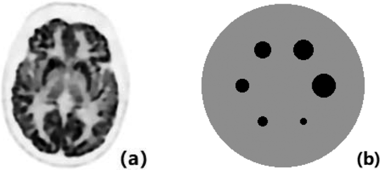
(a) Brain phantom: high quality clinical PET brain image. (b) Uniform phantom: uniform background with six uniform hot spheres of distinct radii.

We show the setting of the regularization parameters and the algorithmic parameters of PKMA in Table 1. For the reconstruction of the brain phantom, to suppress the staircase artifacts and avoid over-smoothed images, we empirically found that setting λ₂ = λ₁ was reasonable and simplified the search for optimal regularization parameters based on the minimum NRMSE. For the uniform phantom, the second-order TV regularization parameters λ₂ was set to 0, due to its piecewise constant nature. The setting of ρ₁ and ρ₂ in PKMA were based on the convergence conditions and the fact that $\Vert {\mathit{B}}_1{\Vert }_2^2\le 8$, $\Vert {\mathit{B}}_2{\Vert }_2^2\le 64$ for the 2D case [34]. The parameters ϱ and δ in the momentum step were set to satisfy that ϱ ∈ (−1, 1) and δ ≥ 0. In addition, we denote by f_UD the uniform disk TMC · 1_disk with the same size as the FOV, where TMC is defined by (28) and 1_disk is the image whose values are 1 within the disk and are 0 outside the disk.

TABLE I.

Regularization Parameters and Algorithmic Parameters for 2D Simulation

Regularization parameters	Brain phantom	High-count: λ1 = λ2 = 0.04 Low-count: λ1 = λ2 = 0.34
	Uniform phantom	High-count: λ1 = 0.4, λ2 = 0
Algoritdmic parameters	PKMA	β = 1, ${\rho }_1=\frac{1}{2\times 8\times S_{\max }}$, ${\rho }_2=\frac{1}{2\times 64\times S_{\max }}$ ϱ = 0.9, δ = 0.1
	PAPA	β = 1, ${\rho }_1=\frac{1}{2\times 8\times S_{\max }}$, ${\rho }_2=\frac{1}{2\times 64\times S_{\max }}$
	ADMM	σ = τ = 0.1, μ = 1.2

B. Simulation Results for IEM-PKMA

1). Comparison of Preconditioners and Momentum Techniques:

In this subsection, we use high-count data to reconstruct the brain phantom for comparison of PKMA with different preconditioners and momentum techniques. The initial image for PKMA was set to f_UD. We show in Fig. 2 the plots of NOFV and NRMSE versus CPU time for PKMA with the EM preconditioner and with four different IEM preconditioners: S_IEM(0), ${\mathit{S}}_{\text{IEM}}({\overline{\mathit{f}}}^{{}^2})$, ${\mathit{S}}_{\text{IEM}}({\overline{\mathit{f}}}^{{}^{20}})$ and ${\mathit{S}}_{\text{IEM}}({\overline{\mathit{f}}}^{{}^{200}})$, where ${\overline{\mathit{f}}}^{{}^2}$, ${\overline{\mathit{f}}}^{{}^{20}}$ and ${\overline{\mathit{f}}}^{{}^{200}}$ represent the images reconstructed by EM-PKMA with 2, 20 and 200 iterations respectively. From these figures, we can see that as $\widehat{\mathit{f}}$ in the IEM preconditioner (27) is made closer to the solution f*, the convergence of PKMA with the preconditioner ${\mathit{S}}_{\text{IEM}}(\widehat{\mathit{f}})$ improves. For all the experiments of Fig. 3-12, $\widehat{\mathit{f}}$ in the IEM preconditioner was always set to f_FBP.

Fig. 3.

NOFV (left) and NRMSE (right) versus CPU time by PKMA with IEM, EM and DN preconditioners, FPGA and IEM-PKMA with the Nesterov momentum parameters.

Fig. 12.

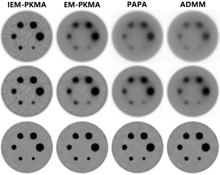
Reconstructed images of the uniform phantom by IEM-PKMA, EM-PKMA, PAPA and ADMM with uniform disk initialization using high-count data: top to bottom rows are reconstructed by 5, 10 and 100 iterations respectively.

In Fig. 3, we compare the results for three different preconditioners: IEM, EM and DN preconditioners, which are defined by (27), (25) and (26) respectively. FPGA and IEM-PKMA with the Nesterov momentum parameters (IEM-PKMA-NM) were also presented. There are two differences between FPGA [24] and IEM-PKMA for model (3), which are the choices of preconditioner and momentum parameters. Specifically, FPGA uses I_d as the preconditioner, while IEM-PKMA uses the IEM preconditioner, and FPGA selects momentum parameters from Nesterov’s update, while we provide a more general form of momentum parameters given by (19) for IEM-PKMA. To compare the performance of our proposed KM based momentum scheme with Nesterov’s, we replace the momentum parameters of IEM-PKMA by (22), yielding a new method we refer to as IEM-PKMA-NM. Optimal step-size β was tuned for each of DN-PKMA (β = 0.3) and FPGA (β = 0.003) based on the performance of objective function value.

In Fig. 4, we present the normalized root mean square difference (NRMSD) $\frac{\Vert {\mathit{f}}_{\text{IEM}}^k-{\mathit{f}}_{\text{DN}}^k{\Vert }_2}{\Vert {\mathit{f}}_{\text{true}}{\Vert }_2}$ between the images reconstructed by IEM-PKMA and DN-PKMA, as well as the reconstructed images with 5000 iterations. This figure shows that the use of two different positive definite preconditioners S_IEM and S_DN give the same converged images.

Fig. 4.

(a) NRMSD between the images reconstructed by IEM-PKMA and DN-PKMA versus iteration number. (b) Reconstructed brain images by IEM-PKMA (left) and DN-PKMA (right) with 5000 iterations.

2). Comparison of Algorithms for SATV Regularization:

In this subsection, we show how IEM-PKMA performs using a smoothed approximation of a first-order edge-preserving regularized model (smoothed anisotropic TV penalty) and compare it to two other state-of-the-art algorithms suitable for smooth penalties. The SATV regularized reconstruction model is given by

$$\underset{\mathit{f}\in {\mathbb{R}}^d}{\text{arg min}}\left\{F(\mathit{f})+\lambda \sum _{j=1}^d\sum _{i\in {\mathcal{N}}_j}{\varphi }_{\theta }(f_j-f_i)\right\},$$ (29)

where F is defined by (2), ${\mathcal{N}}_j$ consists of the indices of both left and up neighbor pixels of the jth pixel of image f, and ϕ_θ is the Lange function [35] defined by

$${\varphi }_{\theta }(t)≔\mid t\mid -\theta \text{ln}\left(1+\frac{\mid t\mid }{\theta }\right),\theta >0.$$

If we let ϕ_θ be the absolute value function, then model (29) becomes the anisotropic TV regularized model. By defining $\mathit{R}(\mathit{f})≔{\sum }_{j=1}^d{\sum }_{i\in {\mathcal{N}}_j}{\varphi }_{\theta }(f_j-f_i)$, IEM-PKMA for solving (29) can be given by

$$\begin{gathered} {\tilde{\mathit{f}}}^{k+1}={\mathit{P}}_{{\mathbb{R}}_{+}^d}\left({\mathit{f}}^k-\beta {\mathit{S}}_{\text{IEM}}(\nabla F({\mathit{f}}^k)+\lambda \nabla R({\mathit{f}}^k))\right) \\ {\mathit{f}}^{k+1}=(1-{\alpha }_k){\mathit{f}}^k+{\alpha }_k{\tilde{\mathit{f}}}^{k+1} \end{gathered}$$

where $\{{\alpha }_k{\}}_{k\in {\mathbb{N}}_0}$ is given by (19). Two state-of-the-art algorithms including OTDA and L-BFGS-B-PC for the SATV regularized model (29) were used for comparison. OTDA is based on the surrogate function method and uses the conjugate direction to accelerate convergence, which has been shown to outperform PCG [8]. L-BFGS-B-PC is based on the quasi-Newton method and uses the diagonal of inverse Hessian matrix for preconditioning. These two algorithms perform well for a differentiable regularization model. However, they both need an additional forward- and back-projection for the line search step, which makes each iteration more time consuming.

Fig. 5 shows the performance of IEM-PKMA, OTDA and L-BFGS-PC for solving model (29) with θ = 0.001 (to ensure edge preservation). High-count data was used and the regularization parameter λ was set to 0.06. For both initialization and the preconditioners in IEM-PKMA and L-BFGS-PC, f_FBP was used.

Fig. 5.

NOFV (left) and NRMSE (right) versus CPU time by IEM-PKMA, OTDA and L-BFGS-B-PC with f_FBP initialization.

3). Comparison of Algorithms for HOTV Regularization:

In this subsection, we compare the performance of PKMA, PAPA and ADMM for the HOTV regularized model. For this purpose, we recall the iteration schemes of PAPA and ADMM. It follows from [3] that PAPA for solving model (3) can be written by

$$\begin{gathered} {\mathit{h}}^k=P_{{\mathbb{R}}_{+}^d}\left({\mathit{f}}^k-\beta {\mathit{S}}_{\text{EM}}(\nabla F({\mathit{f}}^k)+{\mathit{B}}_1^{\mathsf{T}}{\mathit{b}}^k+{\mathit{B}}_2^{\mathsf{T}}{\mathit{c}}^k)\right) \\ {\mathit{b}}^{k+1}={\rho }_1\left(\mathcal{I}-{\text{prox}}_{\frac{{\lambda }_1}{{\rho }_1}{\phi }_1}\right)\left(\frac{1}{{\rho }_1}{\mathit{b}}^k+{\mathit{B}}_1{\mathit{h}}^k\right) \\ {\mathit{c}}^{k+1}={\rho }_2\left(\mathcal{I}-{\text{prox}}_{\frac{{\lambda }_2}{{\rho }_2}{\phi }_2}\right)\left(\frac{1}{{\rho }_2}{\mathit{c}}^k+{\mathit{B}}_2{\mathit{h}}^k\right) \\ {\mathit{f}}^{k+1}=P_{{\mathbb{R}}_{+}^d}\left({\mathit{f}}^k-\beta {\mathit{S}}_{\text{EM}}(\nabla F({\mathit{f}}^k)+{\mathit{B}}_1^{\mathsf{T}}{\mathit{b}}^{k+1}+{\mathit{B}}_2^{\mathsf{T}}{\mathit{c}}^{k+1})\right) \end{gathered}$$

According to [20], ADMM for solving model (3) consists of the following three steps:

$$\{\begin{array}{c}{\mathit{u}}^{k+1}=\underset{\mathit{u}\in {\mathbb{R}}^d}{\text{arg min}}\phi (\mathit{Bu})+\frac{\mu }{2}\Vert {\mathit{f}}^k-\mathit{u}+{\mathit{q}}^k{\Vert }_2^2,\hfill \\ {\mathit{f}}^{k+1}=\underset{f\in {\mathbb{R}}_{+}^d}{\text{arg min}}F(\mathit{f})+\frac{\mu }{2}\Vert \mathit{f}-{\mathit{u}}^{k+1}+{\mathit{q}}^k{\Vert }_2^2,\hfill \\ {\mathit{q}}^{k+1}={\mathit{q}}^k+{\mathit{f}}^{k+1}-{\mathit{u}}^{k+1}.\hfill \end{array}\phantom{\}}$$ (30)

Unlike in [20], the term φ in our model is not differentiable and the proximity operator of φ ∘ B has no explicit form, requiring the first sub-problem of (30) to be solved via the first-order primal-dual algorithm (FOPDA) [36]. Here we perform five FOPDA sub-iterations in each complete ADMM iteration to guarantee the convergence. For the second sub-problem, we use the surrogate function strategy as described in [20].

Then we get the following ADMM iteration scheme:

$$\begin{gathered} {\mathit{b}}^{k,0}={\mathit{b}}^k,{\mathit{c}}^{k,0}={\mathit{c}}^k,{\mathit{u}}^{k,0}={\mathit{u}}^k,{\tilde{\mathit{u}}}^{k,0}={\tilde{\mathit{u}}}^k \\ Forl=1:5 \\ {\mathit{b}}^{k,l}=\sigma (\mathcal{I}-{\text{prox}}_{\frac{{\lambda }_1}{\sigma }{\phi }_1})\left(\frac{1}{\sigma }{\mathit{b}}^{k,l-1}+{\mathit{B}}_1{\tilde{\mathit{u}}}^{k,l-1}\right) \\ {\mathit{c}}^{k,l}=\sigma (\mathcal{I}-{\text{prox}}_{\frac{{\lambda }_2}{\sigma }{\phi }_1})\left(\frac{1}{\sigma }{\mathit{c}}^{k,l-1}+{\mathit{B}}_2{\tilde{\mathit{u}}}^{k,l-1}\right) \\ {\mathit{u}}^{k,l}=\frac{1}{1+\tau \mu }({\mathit{u}}^{k,l-1}-\tau ({\mathit{B}}_1^{\mathsf{T}}{\mathit{b}}^{k,l}+{\mathit{B}}_2^{\mathsf{T}}{\mathit{c}}^{k,l}\phantom{)}+\phantom{(}\tau \mu ({\mathit{f}}^k+{\mathit{q}}^k)) \\ {\tilde{\mathit{u}}}^{k,l}=2{\mathit{u}}^{k,l}-{\mathit{u}}^{k,l-1} \\ End \\ {\mathit{b}}^{k+1}={\mathit{b}}^{k,5},{\mathit{c}}^{k+1}={\mathit{c}}^{k,5},{\mathit{u}}^{k+1}={\mathit{u}}^{k,5},{\tilde{\mathit{u}}}^{k+1}={\tilde{\mathit{u}}}^{k,5} \\ \mathit{w}={\mathit{A}}^{\mathsf{T}}{1}_m-\mu ({\mathit{u}}^{k+1}-{\mathit{q}}^k) \\ \mathit{v}=\text{diag}\{{\mathit{f}}^k\}{\mathit{A}}^{\mathsf{T}}=\frac{\mathit{g}}{A{\mathit{f}}^k+\gamma } \\ {\mathit{f}}^{k=1}=\frac{-\mathit{w}+\sqrt{{\mathit{w}}^2+4\mu \mathit{v}}}{2\mu } \\ {\mathit{q}}^{k+1}={\mathit{q}}^k+{\mathit{f}}^{k+1}-{\mathit{u}}^{k+1} \end{gathered}$$

The choice of parameters in PAPA and ADMM for 2D simulation are shown in table 1. For PAPA, the parameters were chosen according to [3]. For ADMM, the parameters σ and τ were set by the convergence condition $\sigma \tau <\frac{1}{\Vert \mathit{B}{\Vert }_2^2}$ of FOPDA [36], optimal μ was chosen empirically based on the performance of objective function value.

We first show the performance of these algorithms for the reconstruction of the brain phantom using high-count data. Two different initial images, including the uniform disk f_UD and $\widehat{\mathit{f}}$, were used for comparison. Here we set Φ₀ = Φ(f_UD) in the definition of NOFV for both uniform disk and $\widehat{\mathit{f}}$ initialization. In Fig. 6, we show the NOFV and NRMSE versus CPU time by IEM-PKMA, EM-PKMA, PAPA and ADMM with uniform disk and $\widehat{\mathit{f}}$ initialization. It shows that IEM-PKMA converges more rapidly than both PAPA and ADMM. The reconstructed brain images with 5, 10 and 100 iterations in Fig. 7 show that IEM-PKMA is able to obtain a reasonably good image very rapidly. We comment here that the results from the use of IEM preconditioner are more pronounced if a uniform image is used for initialization, and less so when initialized by $\widehat{\mathit{f}}$ in the IEM preconditioner, though still show improvement.

Fig. 6.

NOFV (left) and NRMSE (right) versus CPU time by IEM-PKMA, EM-PKMA, PAPA and ADMM with uniform disk (top row) and $\widehat{f}$ (bottom row) initialization using high-count data.

Fig. 7.

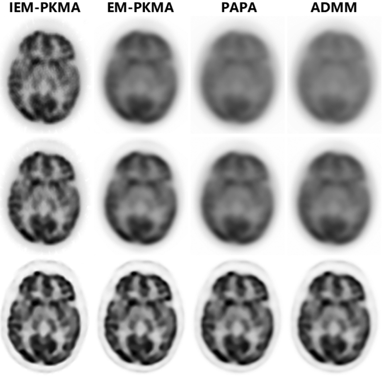
Reconstructed brain images by IEM-PKMA, EM-PKMA, PAPA and ADMM with uniform disk initialization using high-count data: top to bottom rows are reconstructed by 5, 10, and 100 iterations respectively.

To demonstrate the performance of IEM-PKMA for low-count data, we show in Fig. 8 comparisons of NOFV and NRMSE versus CPU time for these algorithms with uniform disk and $\widehat{\mathit{f}}$ initialization. The reconstructed brain images using low-count data are shown in Fig. 9.

Fig. 8.

NOFV (left) and NRMSE (right) versus CPU time by IEM-PKMA, EM-PKMA, PAPA and ADMM with uniform disk (top row) and $\widehat{f}$ (bottom row) initialization using low-count data.

Fig. 9.

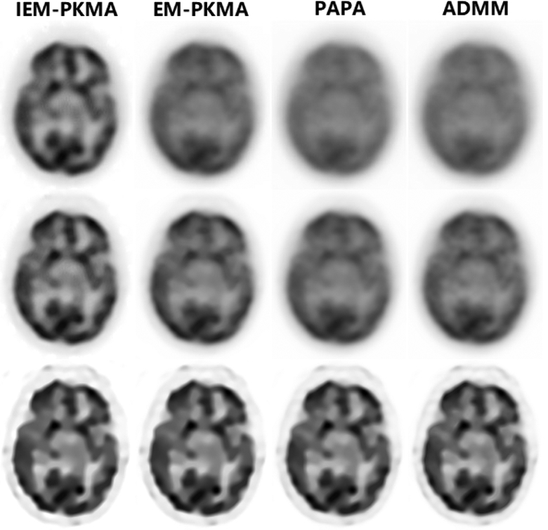
Reconstructed brain images by IEM-PKMA, EM-PKMA, PAPA and ADMM with uniform disk initialization using low-count data: top to bottom rows are reconstructed by 5, 10 and 100 iterations respectively.

We next examine the performance of these algorithms for reconstructing the uniform phantom with uniform disk initialization and high-count data. Fig. 10 shows NRC versus CPU time for the largest and the smallest hot spheres of the uniform phantom. Comparisons of central line profiles of the images reconstructed by 5 and 10 iterations are shown in Fig. 11. The reconstructed images of the uniform phantom are shown in Fig. 12. These figures show that for the uniform phantom, IEM-PKMA outperforms the other algorithms.

Fig. 10.

NRC of the largest hot sphere (left) and the smallest hot sphere (right) versus CPU time by IEM-PKMA, EM-PKMA, PAPA and ADMM with uniform disk initialization using high-count data.

Fig. 11.

CLP of the images reconstructed by 5 iterations (left) and 10 iterations (right) of IEM-PKMA, EM-PKMA, PAPA and ADMM with uniform disk initialization using high-count data.

C. Initial Clinical Results

In this subsection, we present some promising initial 3D clinical results that are based on a relaxed ordered subsets version, ROS-PKMA, according to [31] and [37]. The details of this algorithm and the parameters used are provided in the supplementary materials which are available in the supplementary files tab. We implemented ROS-PKMA, ROS-PAPA [31] and ROS-EM algorithms on a GE D690 PET/CT using a modified version of the GE PET Toolbox release 2.0. A brain scan of 52-year-old male with brain metastases was acquired 1 hour post-injection (370 MBq nominal) for 10 minutes. The images were reconstructed using time-of-flight (TOF) information with a 300 mm FOV using 256 × 256 matrix and an accurate model of the detector PSF (“sharpIR”).

Initial results shown in Fig. 13 appear to indicate that ROS-PKMA with 12 subsets can obtain even better images than both ROS-PAPA and ROS-EM (also with 12 subsets) using only half the iterations.

Fig. 13.

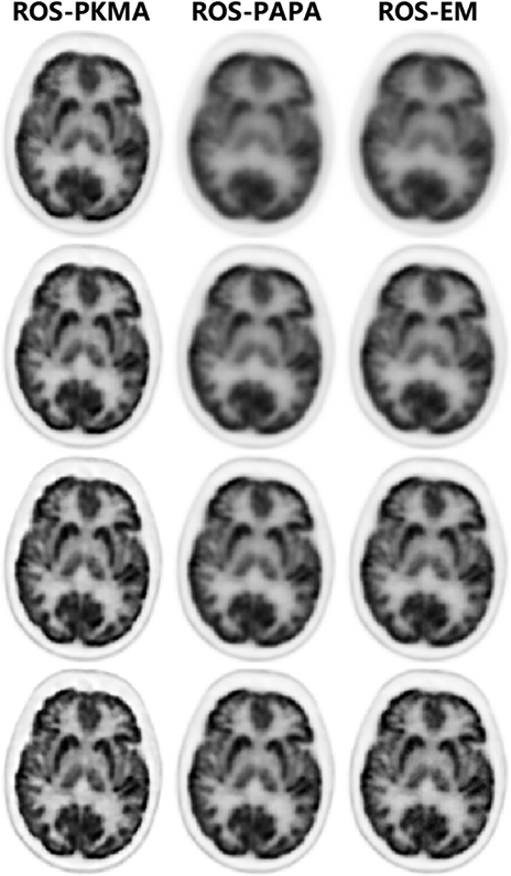
Reconstructed clinical brain images by ROS-PKMA, ROS-PAPA and ROS-EM with 12 subsets: top to bottom rows are reconstructed by 1, 2, 4 and 8 iterations respectively.

IV. Conclusion

This study presents an efficient, easily implemented and mathematically sound preconditioned Krasnoselskii-Mann algorithm for HOTV regularized PET image reconstruction. We prove that PKMA enjoys nice theoretical convergence in the case that the preconditioner is fixed after finite number of iterations. In addition, we show that our proposed generating function for the momentum parameters is more general than the one proposed by Nesterov, able to include both the momentum-free case and an asymptotically equivalent form of the Nesterov momentum parameters as special cases. An improved EM preconditioner that can avoid the reconstructed images being “stuck at zero,” was proposed for accelerating convergence. Numerical experiments demonstrate that the IEM preconditioner improves convergence speed more than the classical EM preconditioner, IEM-PKMA outperforms OTDA, L-BFGS-B-PC for the SATV regularized model, and PAPA, ADMM for the HOTV regularized model. Moreover, for clinical data, promising initial results indicate that ROS-PKMA may be able to obtain sufficiently converged images more rapidly than both ROS-PAPA and ROS-EM, but more research is necessary to properly evaluate these results.

Appendix A

We provide the definition of 2D first-order and second-order isotropic TV (ITV) and the explicit form of the corresponding functions’ proximity operator. For the 3D case, please refer to [3]. The first-order and second-order ITV can be written as φ₁ ∘ B₁ and φ₂ ∘ B₂ respectively. For the definition of B₁ and B₂, we let $N=\sqrt{d}$, I_N denote the N × N identity matrix, D denote the N × N backward difference matrix such that D_j,j = 1 and D_j,j–1 = −1 for j = 2, 3, … , N, and all other entries of D are zero. Through the matrix Kronecker product ⊗, ${\mathit{B}}_1\in {\mathbb{R}}^{2d\times d}$ and ${\mathit{B}}_2\in {\mathbb{R}}^{4d\times d}$ are defined, respectively, by

$${\mathit{B}}_1≔\left[\begin{array}{c}\hfill {\mathit{I}}_N\otimes \mathit{D}\hfill \\ \hfill \mathit{D}\otimes {\mathit{I}}_N\hfill \end{array}\right]{\mathit{B}}_2≔\left[\begin{array}{c}\hfill {\mathit{I}}_N\otimes (-{\mathit{D}}^{\mathsf{T}}\mathit{D})\hfill \\ \hfill (-{\mathit{D}}^{\mathsf{T}})\otimes \mathit{D}\hfill \\ \hfill (-{\mathit{D}}^{\mathsf{T}}\mathit{D})\otimes {\mathit{I}}_N\hfill \\ \hfill \mathit{D}\otimes (-{\mathit{D}}^{\mathsf{T}})\hfill \end{array}\right].$$

For $\mathit{x}\in {\mathbb{R}}^{2d}$, define ${\phi }_1(\mathit{x})≔{\sum }_{i=1}^d\Vert {\mathit{z}}_1^{(i)}{\Vert }_2$, where

$$z_1^{(i)}≔[x_i,x_{d+i}{]}^{\mathsf{T}},i=1,2,\dots ,d.$$ (31)

For $\mathit{x}\in {\mathbb{R}}^{4d}$, define ${\phi }_2(\mathit{x})≔{\sum }_{i=1}^d\Vert {\mathit{z}}_2^{(i)}{\Vert }_2$, where

$$z_2^{(i)}≔[x_i,x_{d+i},x_{2d+i},x_{3d+i}{]}^{\mathsf{T}},i=1,2,\dots ,d.$$ (32)

Next, we provide explicit forms of the proximity operator of φ₁ and φ₂. Let ω be a positive number. As shown in [3], for $\mathit{x}\in {\mathbb{R}}^{2d}$, by denoting u := prox_ωφ1 (x), we have

$$u_{jd+i}=\left(\max \left\{\Vert z_1^{(i)}{\Vert }_2-\omega ,0\right\}∕\Vert z_1^{(i)}{\Vert }_2\right)\cdot x_{jd+i}$$

for j = 0, 1, i = 1, 2,…, d, where ${\mathit{z}}_1^{(i)}$ is defined by (31). For $\mathit{x}\in {\mathbb{R}}^{4d}$, we denote v := prox_ωφ2(x). Then

$$v_{jd+i}=\left(\max \left\{\Vert z_2^{(i)}{\Vert }_2-\omega ,0\right\}∕\Vert z_2^{(i)}{\Vert }_2\right)\cdot x_{jd+i}$$

for j = 0, 1, 2, 3, i = 1, 2, … , d, where ${\mathit{z}}_2^{(i)}$ is defined by (32).

Appendix B

In this appendix, we prove the convergence of PKMA by employing the KM theorem.

To recall the KM theorem, we first recall the definition of nonexpansive operator. Let $\mathit{H}\in {\mathbb{S}}_{+}^n$. We say that $\mathcal{T}:{\mathbb{R}}^n\to {\mathbb{R}}^n$ is nonexpansive with respect to H if for any $\mathit{x}\in {\mathbb{R}}^n$, $\mathit{y}\in {\mathbb{R}}^n$, $\Vert \mathcal{T}\mathit{x}-\mathcal{T}\mathit{y}{\Vert }_{\mathit{H}}\le \Vert \mathit{x}-\mathit{y}{\Vert }_{\mathit{H}}$.

Theorem 4 (Krasnoselskii-Mann [38]-[40]): Let $\mathcal{T}:{\mathbb{R}}^n\to {\mathbb{R}}^n$ be a nonexpansive operator such that the set of its fixed points is non-empty. For $\{{\omega }_k{\}}_{k\in {\mathbb{N}}_0}\subset (0,1)$ and $x^0\in {\mathbb{R}}^n$, define

$${\mathit{x}}^{k+1}=(1-{\omega }_k){\mathit{x}}^k+{\omega }_k\mathcal{T}{\mathit{x}}^k,k\in {\mathbb{N}}_0.$$ (33)

If ${\sum }_{k=0}^{\infty }{\omega }_k(1-{\omega }_k)=+\infty$, then $\{{\mathit{x}}^k{\}}_{k\in {\mathbb{N}}_0}$ converges to a fixed-point of $\mathcal{T}$.

We shall employ Theorem 4 to prove the convergence of PKMA. For this purpose, we rewrite iteration (21) in the form of (33). To this end, we first prove that ${\mathcal{T}}_W$ is averaged nonexpansive with respect to R⁻¹ G. We recall the definition of firmly nonexpansive and averaged nonexpansive operators, and two related lemmas.

An operator $\mathcal{T}:{\mathbb{R}}^n\to {\mathbb{R}}^n$ is called firmly nonexpansive with respect to $\mathit{H}\in {\mathbb{S}}_{+}^n$ if $\Vert \mathcal{T}\mathit{x}-\mathcal{T}\mathit{y}{\Vert }_{\mathit{H}}^2\le \langle \mathcal{T}\mathit{x}-\mathcal{T}\mathit{y},\mathit{x}-\mathit{y}{\rangle }_{\mathit{H}}$ for any $\mathit{x}\in {\mathbb{R}}^n$, $\mathit{y}\in {\mathbb{R}}^n$. If there exists a nonexpansive operator $\mathcal{N}:{\mathbb{R}}^n\to {\mathbb{R}}^n$ with respect to H such that $\mathcal{T}=(1-\alpha )\mathcal{I}+\alpha \mathcal{N}$, we say that $\mathcal{T}$ is α-averaged nonexpansive with respect to H. Firmly nonexpansiveness of an operator corresponds to its $\frac{1}{2}$-averaged nonexpansiveness by [41, Remark 4.24].

Lemma 5 (Baillon-Haddad [41]): Let $\psi :{\mathbb{R}}^n\to \mathbb{R}$ be differentiable and convex, L be a positive real number. Then ∇ψ is L-Lipschitz continuous if and only if for all x, $\mathit{y}\in {\mathbb{R}}^n$, $\Vert \nabla \psi (\mathit{x})-\nabla \psi (\mathit{y}){\Vert }_2^2\le \mathit{L}\langle \mathit{x}-\mathit{y}$, $\nabla \psi (\mathit{x})-\nabla \psi (\mathit{y})\rangle$.

Lemma 6 (Combettes-Yamada [42]): Let $\mathit{H}\in {\mathbb{S}}_{+}^n$, 0 < α₁ < 1 and 0 < α₂ < 1. If $T_1:{\mathbb{R}}^n\to {\mathbb{R}}^n$ is α₁-averaged nonexpansive with respect to H, and $T_2:{\mathbb{R}}^n\to {\mathbb{R}}^n$ is α₂-averaged nonexpansive with respect to H, then T₁ ∘ T₂ is $\frac{{\alpha }_1+{\alpha }_2-2{\alpha }_1{\alpha }_2}{1-{\alpha }_1{\alpha }_2}$-averaged nonexpansive with respect to H.

Notice that $\mathit{W}≔{\mathit{R}}^{-1}\mathit{G}=\left[\begin{array}{cc}\hfill {\mathit{P}}^{-1}\hfill & \hfill -{\mathit{B}}^{\mathsf{T}}\hfill \\ \hfill -\mathit{B}\hfill & \hfill {\mathit{Q}}^{-1}\hfill \end{array}\right]$ is symmetric since P, Q are both symmetric. Therefore, $\mathit{W}\in {\mathbb{S}}_{+}^{d+m_0}$ if and only if its smallest eigenvalue λ_W > 0. Next we prove that ${\mathcal{T}}_W$ is averaged nonexpansive with respect to W.

Lemma 7: Let T_G, ${\mathcal{T}}_W$, r, R and G be defined by (13), (14), (9), (10) and (11) respectively, and $\zeta ≔\frac{2{\lambda }_W}{4{\lambda }_W-L}$. If ${\lambda }_W>\frac{L}{2}$, then ${\mathcal{T}}_W$ is ζ-averaged nonexpansive with respect to W.

Proof: ${\lambda }_W>\frac{L}{2}>0$ gives that $\mathit{W}\in {\mathbb{S}}_{+}^{d+m_0}$ and

$$\Vert {\mathit{W}}^{-\frac{1}{2}}{\Vert }_2^2={\lambda }_{\max }({\mathit{W}}^{-1})={\lambda }_{\mathit{W}}^{-1},$$ (34)

where λ_max(W) denotes the largest eigenvalue of W. [24, Lemma 3.2] shows that T_G is firmly nonexpansive with respect to W. Hence it is $\frac{1}{2}$-averaged nonexpansive with respect to W. According to Lemma 6 and the definition of ${\mathcal{T}}_W$, to prove that ${\mathcal{T}}_W$ is averaged nonexpansive with respect to W, it suffices to show that $\mathcal{I}-{\mathit{W}}^{-1}\nabla r$ is averaged nonexpansive with respect to W.

Define $\alpha ≔\frac{L}{2{\lambda }_W}$ and $\mathcal{N}≔\mathcal{I}-\frac{1}{\alpha }{\mathit{W}}^{-1}\nabla r$. Then 0 < α < 1 and $\mathcal{I}-{\mathit{W}}^{-1}\nabla r=(1-\alpha )\mathcal{I}+\alpha \mathcal{N}$. It is easy to verify that r is convex and differentiable with an L-Lipschitz continuous gradient. For w, $\mathit{v}\in {\mathbb{R}}^{d+m_0}$, let z := ∇r (w) – ∇r (v). By (34), Lemma 5 and by $\alpha =\frac{L}{2{\lambda }_W}$, we have that

$$\frac{1}{{\alpha }^2}\Vert {\mathit{W}}^{-\frac{1}{2}}z{\Vert }_2^2\le \frac{1}{{\alpha }^2}\Vert {\mathit{W}}^{-\frac{1}{2}}{\Vert }_2^2\Vert z{\Vert }_2^2\le \frac{2}{\alpha }\langle \mathit{w}-\mathit{v},z\rangle .$$

Hence

$$\begin{gathered} \Vert \mathcal{N}\mathit{w}-\mathcal{N}\mathit{v}{\Vert }_W^2={\Vert (\mathit{w}-\mathit{v})-\frac{1}{\alpha }{W}^{-1}z\Vert }_W^2 \\ =\Vert \mathit{w}-\mathit{v}{\Vert }_W^2+\frac{1}{{\alpha }^2}\Vert W^{-\frac{1}{2}}z{\Vert }_2^2-\frac{2}{\alpha }\langle \mathit{w}-\mathit{v},z\rangle \\ \le \Vert \mathit{w}-\mathit{v}{\Vert }_W^2, \end{gathered}$$

which implies that $\mathcal{N}$ is nonexpansive with respect to W. Thus $\mathcal{I}-{\mathit{W}}^{-1}\nabla r$ is α-averaged nonexpansive with respect to W. Therefore, ${\mathcal{T}}_W=T_{\mathit{G}}\circ (\mathcal{I}-{\mathit{W}}^{-1}\nabla r)$ is ζ-averaged nonexpansive with respect to W by Lemma 6. ■

Now we prove the convergence of iteration (21).

Theorem 8: Let ${\mathcal{T}}_W$, α_k, ${\mathcal{T}}^{{\alpha }_k}$ be defined by (14), (19) and (20) respectively, where ϱ ∈ (−1, 1) and δ ≥ 0. For given ${\mathit{v}}^0\in {\mathbb{R}}^{d+m_0}$, let $\{{\mathit{v}}^k{\}}_{k\in {\mathbb{N}}_0}$ be a sequence generated by iteration (21), and ${\mathit{f}}^k≔[v_1^k,v_2^k,\dots ,v_d^k{]}^{\mathsf{T}}$, $k\in {\mathbb{N}}_0$. If ${\lambda }_W>\frac{L}{2(1-\max \{\varrho ,0\})}$, then $\{{\mathit{f}}^k{\}}_{k\in {\mathbb{N}}_0}$ converges to a solution of model (5).

Proof: We shall employ Theorem 4 to prove this theorem. To this end, we define $\zeta ≔\frac{2{\lambda }_W}{4{\lambda }_W-L}$, and show below that there exists a nonexpansive operator $\mathcal{N}$ with respect to W such that

$${\mathcal{T}}^{{\alpha }_k}=(1-{\alpha }_k\zeta )\mathcal{I}+{\alpha }_k\zeta \mathcal{N},k\in {\mathbb{N}}_0,$$ (35)

and

$${\alpha }_k\zeta \in (0,1),\sum _{k=0}^{\infty }{\alpha }_k\zeta (1-{\alpha }_k\zeta )=+\infty .$$ (36)

It follows from Lemma 7 that ${\mathcal{T}}_W$ is ζ-averaged nonexpansive with respect to W. By the definition of averaged nonexpansiveness, there exists a nonexpansive operator $\mathcal{N}$ with respect to W such that ${\mathcal{T}}_W=(1-\zeta )\mathcal{I}+\zeta \mathcal{N}$. Substituting this equation into the definition (20) of ${\mathcal{T}}^{{\alpha }_k}$, we obtain (35).

It remains to verify that α_kζ satisfies (36) for $k\in {\mathbb{N}}_0$. If −1 < ϱ < 0, then ${\lambda }_W>\frac{L}{2}$ and 1 + ϱ ≤ α_k ≤ 1, $k\in {\mathbb{N}}_0$. Hence $\frac{1}{2}<\zeta <1$ and $0<\frac{1+\varrho }{2}<{\alpha }_k\zeta \le \zeta <1$, $k\in {\mathbb{N}}_0$. In this case, ${\sum }_{k=0}^{\infty }{\alpha }_k\zeta (1-{\alpha }_k\zeta )>{\sum }_{k=1}^{\infty }\frac{1+\varrho }{2}(1-\zeta )=+\infty$. If 0 ≤ ϱ < 1, then ${\lambda }_W>\frac{L}{2(1-\varrho )}$ and 1 ≤ α_k ≤ 1 + ϱ, $k\in {\mathbb{N}}_0$. Hence $\frac{1}{2}<\zeta <\frac{1}{1+\varrho }$ and $\frac{1}{2}<{\alpha }_k\zeta <1$, $k\in {\mathbb{N}}_0$. Given ζ, 0 ≤ ϱ < 1 implies that there exists ϱ′ such that ϱ < ϱ′ < 1 and $\frac{1}{2}<\zeta <\frac{1}{1+{\varrho }^{\prime }}$. Thus ${\alpha }_k\zeta <\frac{1+\varrho }{1+{\varrho }^{\prime }}$, and then ${\sum }_{k=0}^{\infty }{\alpha }_k\zeta (1-{\alpha }_k\zeta )>{\sum }_{k=0}^{\infty }\frac{1}{2}\left(1-\frac{1+\varrho }{1+{\varrho }^{\prime }}\right)=+\infty$.

Therefore, by Theorem 4, $\{{\mathit{v}}^k{\}}_{k\in {\mathbb{N}}_0}$ converges to a fixed-point of ${\mathcal{T}}_W$. By Theorem 1, we conclude that $\{{\mathit{f}}^k{\}}_{k\in {\mathbb{N}}_0}$ converges to a solution of model (5). ■

For specific choice of the preconditioning matrices P and Q, we have the following lemma for proving the convergence of PKMA.

Lemma 9: Let β, ρ₁, ρ₂ and ξ be positive numbers, $\mathit{S}\in {\mathbb{R}}^{d\times d}$ be a diagonal matrix with positive diagonal entries, P := βS, Q := diag(ρ₁1_m1, ρ₂1_m2), $p≔\frac{1}{\beta S_{max}}$, $\mathit{B}≔\left[\begin{array}{c}\hfill {\mathit{B}}_1\hfill \\ \hfill {\mathit{B}}_2\hfill \end{array}\right]$, and $\mathit{W}≔\left[\begin{array}{cc}\hfill {\mathit{P}}^{-1}\hfill & \hfill -{\mathit{B}}^{\mathsf{T}}\hfill \\ \hfill -\mathit{B}\hfill & \hfill {\mathit{Q}}^{-1}\hfill \end{array}\right]$. If $\beta <\frac{1}{\xi S_{max}}$, ${\rho }_1<\frac{p-\xi }{2\Vert {\mathit{B}}_1{\Vert }_2^2+(p-\xi )\xi }$ and ${\rho }_2<\frac{p-\xi }{2\Vert {\mathit{B}}_2{\Vert }_2^2+(p-\xi )\xi }$, then λ_W > ξ.

Proof: Clearly, W is symmetric. To prove that λ_W > ξ, it suffices to show that

$$W-\xi {\mathit{I}}_{d+m_0}=\left[\begin{array}{cc}\hfill {\mathit{P}}^{-1}-\xi {\mathit{I}}_d\hfill & \hfill -{\mathit{B}}^{\mathsf{T}}\hfill \\ \hfill -\mathit{B}\hfill & \hfill {\mathit{Q}}^{-1}-\xi {\mathit{I}}_{m_0}\hfill \end{array}\right]$$

is positive definite. Let $t_1≔{\left(\frac{1}{{\rho }_1}-\xi \right)}^{-1}$, $t_2≔{\left(\frac{1}{{\rho }_2}-\xi \right)}^{-1}$. If β, ρ₁ and ρ₂ satisfy the conditions in this lemma, then p – ξ > 0, $0<t_1<\frac{p-\xi }{2\Vert {\mathit{B}}_1{\Vert }_2^2}$, $0<t_2<\frac{p-\xi }{2\Vert {\mathit{B}}_2{\Vert }_2^2}$, and moreover, P⁻¹–ξI_d and Q⁻¹–ξI_m0 are both positive definite. Define

$$\tilde{\mathit{B}}≔({\mathit{Q}}^{-1}-\xi {\mathit{I}}_{m_0}{)}^{-\frac{1}{2}}\mathit{B}({\mathit{P}}^{-1}-\xi {\mathit{I}}_d{)}^{-\frac{1}{2}}.$$

Then

$$\tilde{\mathit{B}}=\left[\begin{array}{c}\hfill \sqrt{t_1}{\mathit{B}}_1({\mathit{P}}^{-1}-\xi {\mathit{I}}_d{)}^{-\frac{1}{2}}\hfill \\ \hfill \sqrt{t_2}{\mathit{B}}_2({\mathit{P}}^{-1}-\xi {\mathit{I}}_d{)}^{-\frac{1}{2}}\hfill \end{array}\right]$$

by the definitions of Q and B. It follows from [25, Lemma 6.2] that W – ξI_d+m0 is positive definite if and only if $\Vert \tilde{\mathit{B}}{\Vert }_2<1$, which we verify below. For any ${\mathit{E}}_1\in {\mathbb{R}}^{m_1\times d}$ and ${\mathit{E}}_2\in {\mathbb{R}}^{m_2\times d}$, by the definition of matrix ℓ₂ norm, we have

$$\begin{gathered} {\Vert \left[\begin{array}{c}\hfill {\mathit{E}}_1\hfill \\ \hfill {\mathit{E}}_2\hfill \end{array}\right]\Vert }_2^2=\underset{\Vert x{\Vert }_2=1}{\max }{\Vert \left[\begin{array}{c}\hfill {\mathit{E}}_1\mathit{x}\hfill \\ \hfill {\mathit{E}}_2\mathit{x}\hfill \end{array}\right]\Vert }_2^2 \\ \le \underset{\Vert x{\Vert }_2=1}{\max }\Vert {\mathit{E}}_1\mathit{x}{\Vert }_2^2+\underset{\Vert y{\Vert }_2=1}{\max }\Vert {\mathit{E}}_2\mathit{y}{\Vert }_2^2 \\ =\Vert {\mathit{E}}_1{\Vert }_2^2+\Vert {\mathit{E}}_2{\Vert }_2^2. \end{gathered}$$

Thus

$$\begin{gathered} \Vert \tilde{\mathit{B}}{\Vert }_2^2\le t_1\Vert {\mathit{B}}_1({\mathit{P}}^{-1}-\xi {\mathit{I}}_d{)}^{-\frac{1}{2}}{\Vert }_2^2+t_2\Vert {\mathit{B}}_2({\mathit{P}}^{-1}-\xi {\mathit{I}}_d{)}^{-\frac{1}{2}}{\Vert }_2^2 \\ \le t_1\Vert {\mathit{B}}_1{\Vert }_2^2\cdot (p-\xi {)}^{-1}+t_2\Vert {\mathit{B}}_2{\Vert }_2^2\cdot (p-\xi {)}^{-1} \\ <\frac{1}{2}+\frac{1}{2}=1, \end{gathered}$$

which completes the proof.

References

- [1].Rudin LI, Osher S, and Fatemi E, “Nonlinear total variation based noise removal algorithms,” Phys. D, Nonlinear Phenomena, vol. 60, nos. 1–4, pp. 259–268, 1992. [Google Scholar]
- [2].Bredies K, Kunisch K, and Pock T, “Total generalized variation,” SIAM J. Imag. Sci, vol. 3, no. 3, pp. 492–526, 2010. [Google Scholar]
- [3].Li S et al. , “Effective noise-suppressed and artifact-reduced reconstruction of SPECT data using a preconditioned alternating projection algorithm,” Med. Phys, vol. 42, no. 8, pp. 4872–4887, 2015. [DOI] [PMC free article] [PubMed] [Google Scholar]
- [4].Fessler JA and Booth SD, “Conjugate-gradient preconditioning methods for shift-variant PET image reconstruction,” IEEE Trans. Image Process, vol. 8, no. 5, pp. 688–699, May 1999. [DOI] [PubMed] [Google Scholar]
- [5].Yu DF and Fessler JA, “Edge-preserving tomographic reconstruction with nonlocal regularization,” IEEE Trans. Med. Imag, vol. 21, no. 2, pp. 159–173, February 2002. [DOI] [PubMed] [Google Scholar]
- [6].Wang G and Qi J, “Penalized likelihood PET image reconstruction using patch-based edge-preserving regularization,” IEEE Trans. Med. Imag, vol. 31, no. 12, pp. 2194–2204, December 2012. [DOI] [PMC free article] [PubMed] [Google Scholar]
- [7].Tsai Y-J et al. , “Fast quasi-Newton algorithms for penalized reconstruction in emission tomography and further improvements via preconditioning,” IEEE Trans. Med. Imag, vol. 37, no. 4, pp. 1000–1010, April 2018. [DOI] [PubMed] [Google Scholar]
- [8].Wang G and Qi J, “Edge-preserving PET image reconstruction using trust optimization transfer,” IEEE Trans. Med. Imag, vol. 34, no. 4, pp. 930–939, April 2015. [DOI] [PMC free article] [PubMed] [Google Scholar]
- [9].Panin VY, Zeng GL, and Gullberg GT, “Total variation regulated EM algorithm,” IEEE Trans. Nucl. Sci, vol. 46, no. 6, pp. 2202–2210, December 1999. [Google Scholar]
- [10].Jonsson E, Huang S-C, and Chan T, “Total variation regularization in positron emission tomography,” Univ. California, Los Angeles, Los Angeles, CA, USA, CAM-Rep. 98-48, 1998, pp. 1–25. [Google Scholar]
- [11].Sawatzky A, Brune C, Wubbeling F, Kosters T, Schafers K, and Burger M, “Accurate EM-TV algorithm in PET with low SNR,” in Proc. IEEE Nucl. Sci. Symp. Conf. Rec., October 2008, pp. 5133–5137. [Google Scholar]
- [12].Bardsley JM, “An efficient computational method for total variation-penalized Poisson likelihood estimation,” Inverse Problems Imag, vol. 2, no. 2, pp. 167–185, 2008. [Google Scholar]
- [13].Bardsley JM and Luttman A, “Total variation-penalized Poisson likelihood estimation for ill-posed problems,” Adv. Comput. Math, vol. 31, nos. 1–3, p. 35, 2009. [Google Scholar]
- [14].Bardsley JM and Goldes J, “Regularization parameter selection and an efficient algorithm for total variation-regularized positron emission tomography,” Numer. Algorithms, vol. 57, no. 2, pp. 255–271, 2011. [Google Scholar]
- [15].Chaux C, Pesquet J-C, and Pustelnik N, “Nested iterative algorithms for convex constrained image recovery problems,” SIAM J. Imag. Sci, vol. 2, no. 2, pp. 730–762, 2009. [Google Scholar]
- [16].Bonettini S and Ruggiero V, “An alternating extragradient method for total variation-based image restoration from Poisson data,” Inverse Problems, vol. 27, no. 9, 2011, Art. no. 095001. [Google Scholar]
- [17].Sidky EY, Jørgensen JH, and Pan X, “Convex optimization problem prototyping for image reconstruction in computed tomography with the Chambolle–Pock algorithm,” Phys. Med. Biol, vol. 57, no. 10, p. 3065, 2012. [DOI] [PMC free article] [PubMed] [Google Scholar]
- [18].Komodakis N and Pesquet J-C, “Playing with Duality: An overview of recent primal–dual approaches for solving large-scale optimization problems,” IEEE Signal Process. Mag, vol. 32, no. 6, pp. 31–54, November 2015. [Google Scholar]
- [19].Boyd S, Parikh N, Chu E, Peleato B, and Eckstein J, “Distributed optimization and statistical learning via the alternating direction method of multipliers,” Found. Trends Mach. Learn, vol. 3, no. 1, pp. 1–122, January 2011. [Google Scholar]
- [20].Chun SY, Dewaraja YK, and Fessler JA, “Alternating direction method of multiplier for tomography with nonlocal regularizers,” IEEE Trans. Med. Imag, vol. 33, no. 10, pp. 1960–1968, October 2014. [DOI] [PMC free article] [PubMed] [Google Scholar]
- [21].Krol A, Li S, Shen L, and Xu Y, “Preconditioned alternating projection algorithms for maximum a posteriori ECT reconstruction,” Inverse Problems, vol. 28, no. 11, 2012, Art. no. 115005. [DOI] [PMC free article] [PubMed] [Google Scholar]
- [22].Wu Z, Li S, Zeng X, Xu Y, and Krol A, “Reducing staircasing artifacts in SPECT reconstruction by an infimal convolution regularization,” J. Comput. Math, vol. 34, no. 6, pp. 626–647, 2016. [Google Scholar]
- [23].Pock T and Chambolle A, “Diagonal preconditioning for first order primal-dual algorithms in convex optimization,” in Proc. IEEE Int. Conf. Comput. Vis. (ICCV), November 2011, pp. 1762–1769. [Google Scholar]
- [24].Li Q and Zhang N, “Fast proximity-gradient algorithms for structured convex optimization problems,” Appl. Comput. Harmon. Anal, vol. 41, no. 2, pp. 491–517, 2016. [Google Scholar]
- [25].Li Q, Shen L, Xu Y, and Zhang N, “Multi-step fixed-point proximity algorithms for solving a class of optimization problems arising from image processing,” Adv. Comput. Math, vol. 41, no. 2, pp. 387–422, 2015. [Google Scholar]
- [26].Nesterov YE, “A method of solving a convex programming problem with convergence rate O(1/k2),” Sov. Math. Dokl, vol. 27, no. 2, pp. 372–376, 1983. [Google Scholar]
- [27].Beck A and Teboulle M, “A fast iterative shrinkage-thresholding algorithm for linear inverse problems,” SIAM J. Imag. Sci, vol. 2, no. 1, pp. 183–202, 2009. [Google Scholar]
- [28].Moreau JJ, “Proximité et dualité dans un espace Hilbertien,” Bull. Soc. Math. France, vol. 93, no. 2, pp. 273–299, 1965. [Google Scholar]
- [29].Moreau JJ, “Fonctions convexes duales et points proximaux dans un espace Hilbertien,” C. R. Acad. Sci. Paris A, Math, vol. 255, pp. 2897–2899, December 1962. [Google Scholar]
- [30].Mumcuoglu EU, Leahy R, Cherry SR, and Zhou Z, “Fast gradient-based methods for Bayesian reconstruction of transmission and emission PET images,” IEEE Trans. Med. Imag, vol. 13, no. 4, pp. 687–701, December 1994. [DOI] [PubMed] [Google Scholar]
- [31].Schmidtlein CR et al. , “Relaxed ordered subset preconditioned alternating projection algorithm for PET reconstruction with automated penalty weight selection,” Med. Phys, vol. 44, no. 8, pp. 4083–4097, 2017. [DOI] [PMC free article] [PubMed] [Google Scholar]
- [32].Moses WW, “Fundamental limits of spatial resolution in PET,” Nucl. Instrum. Methods Phys. Res. A, Accel. Spectrom. Detect. Assoc. Equip, vol. 648, pp. S236–S240, August 2011. [DOI] [PMC free article] [PubMed] [Google Scholar]
- [33].Berthon B et al. , “PETSTEP: Generation of synthetic PET lesions for fast evaluation of segmentation methods,” Phys. Med, vol. 31, no. 8, pp. 969–980, 2015. [DOI] [PMC free article] [PubMed] [Google Scholar]
- [34].Micchelli CA, Shen L, and Xu Y, “Proximity algorithms for image models: Denoising,” Inverse Problems, vol. 27, no. 4, 2011, Art. no. 045009. [Google Scholar]
- [35].Lange K, “Convergence of EM image reconstruction algorithms with Gibbs smoothing,” IEEE Trans. Med. Imag, vol. 9, no. 4, pp. 439–446, December 1990. [DOI] [PubMed] [Google Scholar]
- [36].Chambolle A and Pock T, “A first-order primal-dual algorithm for convex problems with applications to imaging,” J. Math. Imag. Vis, vol. 40, no. 1, pp. 120–145, 2011. [Google Scholar]
- [37].Kim D, Ramani S, and Fessler JA, “Combining ordered subsets and momentum for accelerated X-ray CT image reconstruction,” IEEE Trans. Med. Imag, vol. 34, no. 1, pp. 167–178, January 2015. [DOI] [PMC free article] [PubMed] [Google Scholar]
- [38].Krasnosel’skii MA, “Two remarks on the method of successive approximations,” Uspekhi Matematicheskikh Nauk, vol. 10, no. 1, pp. 123–127, 1955. [Google Scholar]
- [39].Mann WR, “Mean value methods in iteration,” Proc. Amer. Math. Soc, vol. 4, no. 3, pp. 506–510, 1953. [Google Scholar]
- [40].Bauschke HH and Combettes PL, Convex Analysis and Monotone Operator Theory in Hilbert Spaces. New York, NY, USA: Springer, 2011. [Google Scholar]
- [41].Baillon J-B and Haddad G, “Quelques propriétés des opérateurs anglebornés etn-cycliquement monotones,” Isr. J. Math, vol. 26, no. 2, pp. 137–150, 1977. [Google Scholar]
- [42].Combettes PL and Yamada I, “Compositions and convex combinations of averaged nonexpansive operators,” J. Math. Anal. Appl, vol. 425, no. 1, pp. 55–70, 2015. [Google Scholar]
Associated Data
This section collects any data citations, data availability statements, or supplementary materials included in this article.