Abstract
The COVID-19 outbreak is deeply influencing the global social and economic framework, due to restrictive measures adopted worldwide by governments to counteract the pandemic contagion. In multi-region areas such as Italy, where the contagion peak has been reached, it is crucial to find targeted and coordinated optimal exit and restarting strategies on a regional basis to effectively cope with possible onset of further epidemic waves, while efficiently returning the economic activities to their standard level of intensity.
Differently from the related literature, where modeling and controlling the pandemic contagion is typically addressed on a national basis, this paper proposes an optimal control approach that supports governments in defining the most effective strategies to be adopted during post-lockdown mitigation phases in a multi-region scenario. Based on the joint use of a non-linear Model Predictive Control scheme and a modified Susceptible-Infected-Recovered (SIR)-based epidemiological model, the approach is aimed at minimizing the cost of the so-called non-pharmaceutical interventions (that is, mitigation strategies), while ensuring that the capacity of the network of regional healthcare systems is not violated. In addition, the proposed approach supports policy makers in taking targeted intervention decisions on different regions by an integrated and structured model, thus both respecting the specific regional health systems characteristics and improving the system-wide performance by avoiding uncoordinated actions of the regions.
The methodology is tested on the COVID-19 outbreak data related to the network of Italian regions, showing its effectiveness in properly supporting the definition of effective regional strategies for managing the COVID-19 diffusion.
Keywords: COVID-19, Pandemic modeling, SIR model, Multi-region SIR model, Epidemic control, Post-lockdown mitigation strategies, MPC
1. Introduction and paper positioning
On December 31, 2019, the Wuhan Municipal Health Commission (China) reported to the World Health Organization a cluster of pneumonia cases of unknown etiology in the city of Wuhan, in the Chinese province of Hubei. On January 9, 2020, the Chinese Center for Disease Control and Prevention reported that a new coronavirus (SARS-CoV-2, later called COVID-19) was identified as the cause of such respiratory diseases. On March 11, 2020, the World Health Organization declared the COVID-19 viral disease a pandemic. Since then, the COVID-19 has affected the whole world, with about ten millions of confirmed cases and five hundred thousand of confirmed deaths up to August 2020 over more than two hundred countries, areas, or territories, thus becoming one of the most relevant pandemics in the recent decades (World Health Organization, 2020). Like other Coronaviruses (e.g., SARS and MERS), the COVID-19 appears to be controllable using basic Non-Pharmaceutical Interventions (NPIs), particularly social-distancing and the use of face-masks in public (especially when implemented in combinations). The factors that are obviously critically-important to the success of the anti-COVID-19 control efforts are the early implementation (and enhancement of effectiveness) of these measures, and ensuring their high adherence/coverage in the community (Ngonghala et al., 2020). However, despite the adoption of these measures, it is still possible that secondary waves of contagion occur. For instance, in China, restrictions were eased as cases declined, but by mid May, 2020, new clusters were reported, including in the city of Wuhan where the virus first emerged. In effect, although the adopted countermeasures appear to have reduced the number of reported cases, the absence of herd immunity against COVID-19 suggests that contagions could easily rise again when these interventions are relaxed, as business, factory operations, and schools resume (Leung et al., 2020).
As a consequence, in recent months there has been a growing research interest on COVID-19 mitigation in different scientific fields. One of the most investigated research area aims at developing dynamical models to predict the evolution of the pandemic (Hernandez-Vargas, Alanis, and Tetteh, 2019). In effect, predicting the trend of the epidemic is of paramount importance to plan effective control strategies (Giordano et al., 2020) to limit or block the spread of the epidemic. Broadly speaking, since a vaccine is not yet available, two main control strategies can be applied (Ferguson et al., 2020, Casella, 2021): (1) mitigation, consisting in slowing but not necessarily stopping the epidemic spread (e.g., through isolation of suspect cases and social distancing of the elderly), so that the peak healthcare demand is reduced and individuals that are most at risk of severe disease from infection can be protected, and (2) suppression, which is aimed at reversing the epidemic growth, so that the number of cases is reduced, and kept low. Clearly, each strategy has its own advantages and drawbacks, and the choice among the possible actions mainly relies on economic and social reasons, which slightly differ from country to country (Ferguson et al., 2020). For instance, most countries have attempted to control the effect of COVID-19 by adopting a total lockdown of their population at a relevant economic cost, while few other countries have preferred timed interventions aimed at reducing the number of infected people to a manageable level, depending on the capacity of the healthcare system to absorb and treat the newly infected (Bin et al., 2020). In this regard, it is evident that the proper selection of which strategic action (or which combination of them) should be adopted to ensure the best outcomes is a challenging task.
In the pertinent literature, several models have been developed to describe the pandemic dynamics, which are based on the classic compartmental epidemiological models (Hethcote, 2000, Nowzari, Preciado, and Pappas, 2016), and adapting them to the specific case of COVID-19. Briefly said, epidemiological models, describing disease transmission within a population, provide important insights to understand which control mechanisms can lead, under what circumstances, to remove, or at least reduce, the infection (Mei, Mohagheghi, Zampieri, and Bullo, 2017). More in detail, according to the work in Hethcote (2000), compartmental epidemiological models are typically classified on the basis of the considered compartments of individuals and the related flow patterns. In particular, labels such as M (i.e., infants with passive immunity), S (that is, the class of Susceptible people, i.e., those who can become infected), E (the class of Exposed, i.e., those who are infected but not yet infectious), I (the class of Infective individuals,i.e., those who are capable of transmitting the infection), and R (the Recovered class, i.e., those with permanent infection-acquired immunity) are often used for epidemiological classes, and the threshold for most epidemiological models is the basic reproduction number R 0, defined as the average number of secondary infections produced when one infected individual is introduced into a population of Susceptible individuals (Hethcote, 2000). Depending on the specific features of the disease to be modeled, some of the above compartments can be omitted (as an example, as shown in Ridenhour, Kowalik, and Shay (2018), the Exposed compartment is generally used only when the disease has a significant latent period relative to the infectious period), as well as further compartments can be identified and represented, nevertheless three of the recalled compartments should be always included in the model, that is Susceptible, Infective, and Recovered compartments; consequently all these models fall into the broader class of the so-called SIR-based epidemiological models. Referring to COVID-19, an example of a variant of the classic SIR model is presented in Calafiore, Novara, and Possieri (2020), while SEIR models are proposed in Casella (2021) and in Gatto et al. (2020).
In the case COVID-19 it is necessary to consider particularly detailed models to accurately predict the dynamics of the epidemic (Giordano et al., 2020, Nowzari et al., 2016). In effect, COVID-19 presents four main peculiarities that are difficult to describe with the classic epidemiological models (Zhao and Chen, 2020): 1) the spread of the pandemic has impacted the global population and the respective complex healthcare and economic systems; 2) due to a large incubation period (which may be of two weeks even), differences between the real dynamics and the daily observed number of cases may be observed; 3) multiple factors should be explicitly modeled, such as local medical resources and quarantine measures; 4) since quarantine measures are widely implemented, a lower chance to infect the Susceptible individuals is to be modeled. Therefore, more classes have been introduced in the recent studies on COVID-19 predictive models. For instance, a SUQC model (that is, with Susceptible, Un-quarantined infected, Quarantined infected, and Confirmed infected classes) is proposed in Zhao and Chen (2020) to describe the COVID-19 dynamics in China and analyze the effects of some control measures. A SIDARTHE model is proposed in Giordano et al. (2020), where the population is divided into eight classes: S (Susceptible), I (Infected), D (Diagnosed, that is, detected asymptomatic infected); A (Ailing, that is, undetected symptomatic infected), R (Recognized, that is, detected symptomatic infected), T (Threatened, i.e., detected infected with life-threatening symptoms), H (Healed, i.e., recovered), and E (Extinct, i.e., dead). The final goal of the contribution in Giordano et al. (2020) is to estimate the impact of different actions to contain the contagion in Italy. To this aim, the authors evaluate different possible scenarios by suitably modifying some model parameters.
The recalled works focus on the analysis of the COVID-19 in a country at a national level; however, given the heterogeneity of economic and social features at regional level in almost any country, and particularly in Italy, it is actually essential to assess the evolution of the pandemic when applying suitable local post-lockdown strategies (that is, once the epidemic is brought under control, or in the so-called Phase 2). In effect, many countries are divided into administrative regions which can independently oversee their own share of national healthcare system (Della Rossa, Salzano, Di Meglio et al., 2020). Nonetheless, only few contributions in the related literature take into account the spatial dynamics of the epidemic, among which we recall the work in Gatto et al. (2020), where a spatial SEIR model for the ongoing COVID-19 emergency in Italy is developed as a baseline support tool to plan the inter-regional mobility and to deploy medical supplies and staff based on the local epidemiological conditions. Similarly, in Di Domenico, Pullano, Coletti, Hens, and Colizza (2020) a SEIIR model (i.e., including classes of Susceptible, Exposed, pre-symptomatic and symptomatic Infectious, and Removed individuals) is adopted to evaluate the impact of school closure and telework during the COVID-19 lockdown in the three most affected France regions (i.e., le-de-France, Hauts-de-France, Grand Est) through a stochastic age-structured data-driven analysis. A generalized multi-region SIR model is proposed in Brugnano and Iavernaro (2020), as well as a multi-region SI 2 R 2 extension (where the considered classes are Susceptible, Infectious but not yet diagnosed, Infectious diagnosed, Removed undiagnosed, and Removed diagnosed individuals), albeit only the mathematical formulation of the models is reported while the validation is not yet available. Finally, in Della Rossa et al. (2020) a model including the Susceptible, Infected, Quarantined, Hospitalized, Recovered, and Deceased compartments for the Italian regions is presented to evaluate the effectiveness and impact level of differentiated but coordinated local actions during Phase 2, to avoid future recurrence of the epidemic, while taking into account the specific regional healthcare systems’ characteristics. The main finding of these studies is that the expected impact of mitigation measures deeply varies across different regions. Therefore, it is essential to correctly parameterize the model to the specific characteristics of each region under examination.
All the above recalled approaches, while being able to model the pandemic dynamics, do not provide a feedback control method to properly select the most beneficial action(s) (for instance, based on the number of infected or of hospitalized patients) to be applied in a post-lockdown framework. In fact, these methods can be classified as open-loop techniques that typically require what-if analyses (through scenario-based evaluations or Monte Carlo simulations) to identify the most effective actions. In this perspective, it is fundamental to provide a tool for a feedback-based selection of the mitigation strategy that continuously adapts to the contagion evolution. This is possible by constantly measuring and monitoring the pandemics values and adapting the policy accordingly (Köhler et al., 2020). It has been proven that an open-loop optimal control policy is successful to evaluate simple policies under the assumption of exact model knowledge, while in a more realistic scenario with uncertain data and model mismatch, a feedback strategy that periodically updates the policy is much more effective (Köhler et al., 2020). In effect, the use of feedback control theory represents a powerful tool to support managing the COVID-19 outbreak (Casella, 2021). Unfortunately, most of the existing literature contributions on the control of previous epidemics involves vaccines or treatments, which are currently not available for COVID-19.
In addition, in the recalled contributions, the lockdown periods are typically driven by a periodic switching logic. On the contrary, in order to ensure an active and effective support to the decision-making process, it is essential to tune the parameters of the mitigation strategy over larger time periods, providing a robust outer supervisory feedback loop to the process (Bin et al., 2020). To this aim, the contribution in Bin et al. (2020) proposes a fast switching policy, consisting in multi-shot interventions based on the outcomes of two SIR-based models (i.e., the SIQR and the SIDARTHE) to switch between quarantine (i.e., social isolation) and work days (that is, normal behavior).
Given the obvious uncertainties in the spreading of the virus and in the disease progression, an effective feedback control strategy can be obtained by joining a SIR-based epidemic model with other techniques, thus providing a hybrid model. In fact, the challenge is to determine the optimal external input across time so that a target can be reached (e.g., by optimizing a cost function) (Sélley, Besenyei, Kiss, and Simon, 2015). Hence, the final aim is to combine a disease transmission model with a feedback control mechanism of the epidemics, which allows controlling the whole network rather than only predicting the recovery time or the proportion of infected individuals. Indeed, optimal control theory has been already successfully applied to identify the best action strategies for other diseases, typically by simply introducing into the predictive model a new control variable representing the vaccination rate at time t (see, e.g., the work in Rodrigues, Monteiro, and Torres (2014), where a SIR model for dengue is proposed, and that in Rachah and Torres (2015), where a SIR model for Ebola is presented), or other specifically defined control variables (such as, for instance, in Silva and Torres (2013), where an ad-hoc model for the optimal control of tuberculosis is suggested by including in the model reinfection and post-exposure interventions).
In this perspective, Model Predictive Control (MPC) is a control technique including both feedback control and optimization that allows to take into account the deviations of the predictive model from the real progress of the disease (Bussell, Dangerfield, Gilligan, and Cunniffe, 2019, Morato, Normey-Rico, and Sename, 2020). Although implementing the MPC controller typically requires a large amount of computational resources, which can lead to long computation time (Carli, Cavone, Dotoli, Epicoco, and Scarabaggio, 2019), this is not a concern when the optimization is performed at a strategic level, as is the case of the decision-making process for the definition of the proper strategies to tackle epidemiological diseases. The basic idea here is to keep the true system state (that is, the predicted future output of the model) in line with the selected target. This is achieved based on past control inputs and the optimal predicted control input over a prediction horizon by solving an optimization problem aimed at minimizing a cost function (Alleman, Torfs, and Nopens, 2020). Basically, at regular time intervals, the values of the state variables in the prediction model are updated, hence the control is re-optimized and the new strategy is applied to the system until the next update time, thus ensuring that the approximate model and the control strategy closely match at each time interval (Bussell et al., 2019). The main strength of this procedure is that it allows to directly take into account the unavoidable uncertainties in the model (Alleman et al., 2020). In effect, MPC has been already applied, in conjunction with some SIR-based predictive model, in some previous studies on epidemiological models, showing that coupling feedback control with simulation models can help designing effective and robust action strategies for managing epidemics (Bussell et al., 2019). For instance, the contribution in Sélley et al. (2015) investigates the dynamical control of a generic SIS (i.e., Susceptible-Infectious-Susceptible) epidemic model through a non-linear MPC method aimed at minimizing an objective function (which includes the predicted future outputs of the model) over a finite predictive horizon (which is moved forward at each control step). The work in Sélley et al. (2015) shows that the MPC algorithm allows to guide the system to the desired target once the values of the control parameters are carefully chosen. A robust economic MPC for the containment of a generic stochastic SEIV (i.e., Susceptible-Exposed-Infected-Vigilant) epidemic process is presented in Watkins, Nowzari, and Pappas (2019), with the final aim of deciding who to quarantine, and for how long, in the presence of an epidemic contagion. Furthermore, the work in Bussell et al. (2019) studies a generic stochastic SIR model to optimally allocate vaccination resources while minimizing the costs of an epidemics, showing that the use of MPC allows improving the disease management, reducing cost, and ensuring more robustness to uncertainty, thus performing well on complex models.
In the COVID-19 framework, to the best of the authors’ knowledge, the joint use of predictive epidemiological models and MPC has been studied in just very few papers. More in detail, the work in Alleman et al. (2020) proposes a methodology based on an extended SEIR-model and MPC to determine the optimal government strategy to tackle the COVID-19 in Belgium under dynamic circumstances. First, the model is calibrated by means of the available data over time on the number of active cases and that of deaths. Then, the MPC is used to optimize the time course of social measures with respect to the available Intensive Care Units under three different scenarios: no government action; the current policy (i.e., with mild social restrictions); on-off strategy and immunization of the herd. Similarly, the contribution in Köhler et al. (2020) combines a SIDARTHE model and a robust MPC approach that adapts the social distancing measures to minimize the number of fatalities over a range of two years when measurements are inaccurate and infection rates cannot be precisely evaluated. First, the model parameters and the initial conditions are calibrated according to the COVID-19 outbreak in Germany. Then, the outcomes obtained through a closed-loop control via MPC are compared with those obtained when a multi-objective open-loop optimal control is performed, showing that the latter approach may lead to intermediate increases in the number of new infections, thus requiring an additional lockdown period, while the former method is able to avoid such a behavior, thus significantly reducing the number of fatalities.
Against this background, this paper presents a multi-region SIRQTHE model in conjunction with a non-linear MPC approach which is able to simultaneously take into account both the specific strategies undertaken at the regional level (i.e., restrictions on the intra-region activity) and the actions taken at the upper level in terms of border activities between the regions (i.e., restrictions on the inter-region activity). We remark that, in this paper, we refer to the control actions to be undertaken in order to mitigate the effect of secondary waves of pandemic, that is, we are assuming that the basic non-pharmaceutical interventions (such as, for instance, social-distancing and the use of face-masks) have been ineffective or measures have been relaxed, and as such some more restrictive (but still non-pharmaceutical) measures, such as restrictions on the intra-region and on inter-region activities, are needed.
The analysis is conducted in Italy, since this is one of the countries where the pandemic effect has been the most significant, particularly in some regions (such as in Lombardy), as well as diversified in the territory. In addition, the healthcare system is a regionally based national health service (known as Servizio Sanitario Nazionale), in which public healthcare facilities strongly vary in terms of quality depending on the region. The presented approach can be easily applied to different levels of the spatial scale, provided the availability of data to calibrate the model.
With respect to the existing state of the art, the novel contributions of this paper are as follows:
-
•
We define a networked SIR-based model (a SIRQTHE model) to represent the spread of COVID-19 in multi-region areas where the economic and healthcare systems are characterized by strong regional heterogeneity. More in detail, we extend the model proposed by Brugnano and Iavernaro (2020) by defining a more accurate single-region epidemic model, where seven compartments are introduced (namely, Susceptible, Infected, Removed, Quarantined, Threatened, Healed, and Extinct). We remark that, differently from the six-compartment model presented in Della Rossa et al. (2020), in this work we split the compartment of recovered individual into two classes: the class of Healed people (i.e., recognized individuals that heal after transition in the status of Quarantined or Threatened), and that of Removed people (i.e., completely recovered people that have never been detected). However, it is important to remark that, even employing more classes than the model in Della Rossa et al. (2020), our approach has fewer connections between the classes and hence fewer parameters are to be estimated, to the benefit of the model simplicity. Moreover, while in Della Rossa et al. (2020) the model parameters are dynamically identified by splitting the fitting period, in our work we identify time-varying functions to model time-varying parameters, such as the recovery and the death rate. Finally, another improvement with respect to the model presented in Della Rossa et al. (2020) is that we leverage on the Google mobility reports to better take into account the time-dependency of the infection rate.
-
•
While in the related literature modeling and controlling the pandemic contagion is typically addressed on a national basis, this paper proposes an optimal control approach that supports governments in defining the most effective strategies to be adopted during post-lockdown mitigation phases in a diversified multi-region scenario. The proposed approach allows policy makers taking targeted intervention decisions on different regions by an integrated and structured model, thus both respecting the specific regional healthcare systems characteristics and improving the system-wide performance by the avoidance of uncoordinated behavior by individual regions.
-
•
Differently from the related literature, where the addressed control strategies aim at minimizing the number of fatalities or ensuring that the healthcare systems is not overloaded, this paper also focuses on the economic impact of the control strategies. Indeed, the approach aims at minimizing the cost of the mitigation strategies on a multi-region area, while ensuring that the capacity of the network of regional healthcare systems is not violated.
-
•
By applying the proposed methodology to the network of Italian regions, we show its effectiveness and flexibility in properly supporting the definition of effective regional strategies for managing the COVID-19 disease under different government policies. We discuss the results achieved by the MPC scheme when control actions within and on the border of regions are applied both by a region-by-region basis or by an inter-region coordination mechanism. In particular, we analyze and compare the following scenarios: uniform intra-region activity and inter-region travel restrictions, differentiated intra-region activity restrictions and uniform inter-region travel restrictions, and differentiated intra-region activity and inter-region travel restrictions.
The rest of this work is structured as follows. In Section 2, we first present the single-region SIRQTHE model, providing the formulation of the dynamic equations and the description of the parameters’ identification process; subsequently we focus on the extension of the SIRQTHE model to a multi-region framework. In Section 3, we present the multi-region MPC framework, describing the control variables, the corresponding constraints, and the control objectives, and formulating the optimal control problem. In Section 4, we show the numerical results of the simulations of the Italian country based on real data (Italian Civil Protection Department, 2020a) and we provide a comparison with respect to the results obtained by benchmark control strategies. Finally, in Section 5, we conclude the paper and discuss an outlook for future works. The parameters identification procedures for the SIRQTHE model are reported in Appendix A, distinguishing into A.1 that describes the available data for the Italian case, A.2 presenting the parameters identification procedure for the single-region SIRQTHE model, and A.3 presenting the parameters identification procedure for the multi-region SIRQTHE model; while the list of parameters used in the MPC scheme is reported in Appendix B.
2. Model of the COVID-19 dynamics
Currently, governments all around the world are struggling to contain the COVID-19 pandemic. In this context, mathematical models are extremely valuable to simulate and control the spread of the pandemic. In fact, mathematical models are widely used to estimate the contagion parameters and predict the effects of any control action on populations.
2.1. Basics on SIR-based epidemiological models
Compartmental models are traditionally considered suitable to model the spread of a virus within a large population (Hethcote, 2000). In these models, the overall population is divided into different compartments, where people can flow from one compartment to another based on specific rate values. In particular, in the SIR-based models, we can assume that the dynamics of the pandemic is quicker than the dynamics of birth and death, therefore, the latter two events are usually omitted. Hence, the simplest SIR model can be expressed by the following set of ordinary differential equations (Hethcote, 2000):
| (1) |
| (2) |
| (3) |
where N denotes the overall population, S, I, and R represent respectively the compartments of the Susceptible, Infected, and Removed (dead or recovered) individuals, is the infection rate, and is the recovery rate. Since N corresponds to the sum of compartments populations, it holds:
| (4) |
Consequently, in (1)-(3) it is sufficient to analyze only two equations since the third is dependent.
Finally, it is to be noticed that, as an alternative to (1)-(3), the discrete-time version of the SIR can be straightforwardly formulated (since a comparison between the two variants is out of the scope of this contribution, we refer the interested reader to the work in Chen (2019) for details). Independently from the choice of the time domain, the SIR model is able to characterize in broad terms the spread of a pandemic, thus disregarding the multiple and complex facets of a real pandemic. Consequently, several models have been proposed in the related literature to improve the classical SIR model for a specific pandemic, for instance, by adding additional compartments and by better modeling the relation among them.
2.2. Single-region SIRQTHE model
The proposed epidemiological model for the COVID-19 is a novel time-varying discrete-time model, named SIRQTHE, which distinguishes between detected and undetected infected people, healed, dead, and hospitalized. As a major assumption, we suppose that the probability of becoming susceptible after being healed is negligible, which seems reasonable based on the current level of knowledge (Bai et al., 2020).
More in detail, in our model, the overall population in a given region is divided into the following compartments:
-
•
S: Susceptible;
-
•
I: Infected (infected and undetected);
-
•
R: Removed (undetected and completely recovered);
-
•
Q: Quarantined (infected and detected)
-
•
T: Threatened (hospitalized in a life-threatening or noncritical situation);
-
•
H: Healed (completely recovered);
-
•
E: Extinct (dead).
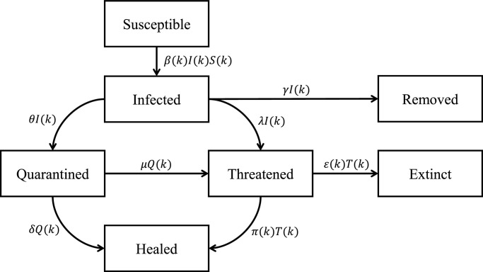
The overall interconnections between the above compartments are shown in Fig. 1 .
Fig. 1.
Scheme of the SIRQTHE model.
The SIRQTHE model is composed by seven time-varying difference equations, which characterize the flows of the individuals between the different compartments. More in detail, by designating all the state variables (the fraction of the overall population) by a Latin letter, and denoting the time step as k, the model is described as follows:
| (5) |
| (6) |
| (7) |
| (8) |
| (9) |
| (10) |
| (11) |
where the state variables indicated with a tilde are those that cannot be directly observed with a reasonable confidence, i.e., there are no data from official sources (Calafiore et al., 2020).
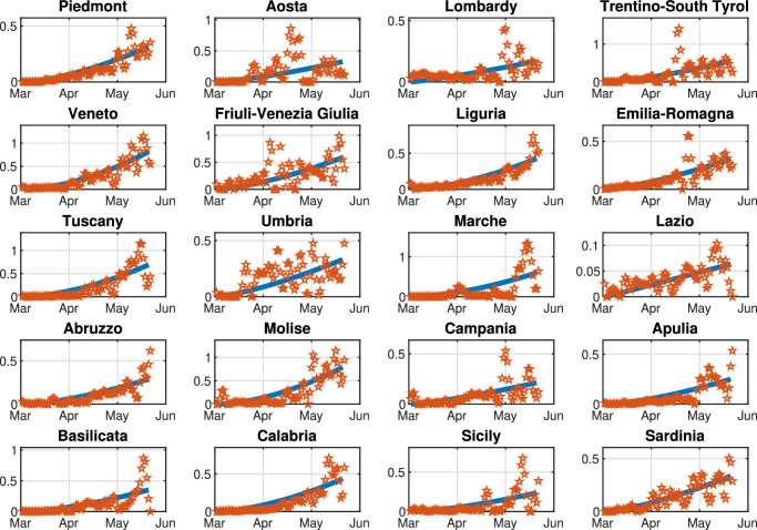
Let us describe in detail the model parameters and the assumptions underlying the model conceptualization. As shown in Fig. 1, the seven classes are related by different parameters, which are able to capture the system dynamics. In particular, β(k) is the time-varying infection rate, whose value is strongly dependent on the population behavior and the social distancing measures. In Appendix A, we show that this parameter may be highly correlated with people’s mobility. Parameter θ is the rate of infected that are recognized and Quarantined, γ is the rate of healing when the Infected and unrecognized people do not need to be hospitalized, δ is the rate of healing of Quarantined people, λ is the rate of people that have been recognized only when a strong symptomatic condition occurs and therefore an immediate hospitalization is needed. Moreover, μ is the rate of Quarantined people that need to be hospitalized, π is the rate of healing of the Threatened people and ε is the death rate.
The justification of this model construction lies in achieving a good compromise between the model accuracy, which allows representing all the facets of the pandemic diffusion, and the simplicity that helps identifying the characteristic parameters from the available data. As shown in Section 1, several papers on the spread of COVID-19 pandemic indeed present compartmental models with more classes; however, these works mainly lack of an accurate identification of the model parameters. In several countries, the available data are scarce and are divided into few categories: this makes a more complex model hardly implementable in real life. As a consequence, some simplifying assumptions must be indeed made for the sake of preserving the model practicality. In reference to the SIRQTHE model, we compress or eliminate some classes that are usually employed in more complex models. For instance, we consider simply a Quarantined people class not discerning from those asymptomatic and those with mild or strong symptoms. Moreover, we ignore that hospitalized individuals may in fact require different treatments; in fact, several models divide this class considering an additional class that takes into account people needing intensive care treatments. In addition, we partially neglect the incubation time of the virus. Lastly, we do not use the so-called Exposed compartment, which contains the people that have been infected while they are not yet contagious. Despite these hypotheses, as shown in Appendix A, the proposed SIRQTHE model shows its effectiveness in the identification phase based on a minimal set of measurable epidemiological data that are commonly available across countries.
2.3. Multi-region SIRQTHE model
In order to correctly represent the COVID-19 spread, a multi-region variant of the model in (5)-(11) is here proposed. In effect, a multi-region model is more reliable than a centralized model to reproduce the heterogeneous situation in multi-region areas with high-fidelity. In particular, as proposed in Brugnano and Iavernaro (2020), we generalize our SIRQTHE model to a multi-region case. By assuming the area under analysis is composed by M regions, whose index i varies in the set the equations related to the i-th region can be written as follows:
| (12) |
| (13) |
| (14) |
| (15) |
| (16) |
| (17) |
| (18) |
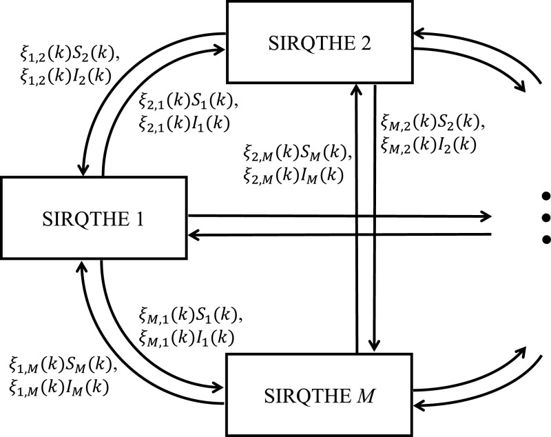
Comparing equations (5)-(11) with (12)-(18), we remark that in the latter formulation we mark the state variables related to region i with the corresponding index, and we add a further term in the right-hand side of the first two difference equations to take the migration of individuals between regions into account. In particular, we use the time-varying coefficients to represent the inter-region mobility: ξ i,j(k) () is the coefficient of migration from region j to region i at time k, whilst ξ i,i(k) represents the rate of people leaving the region i at time k. We assume that all the parameters ξ i,j(k) () get non-negative values; thus, ξ i,i(k) has a non-positive value equal to:
| (19) |
Note that (19) is derived by imposing the balance of the migrations flows between all the regions:
| (20) |
The complete model for a network composed by M regions can be written in matrix form. First we define:
| (21) |
as the vectors containing all the state variables for each region. Then, we define the model parameters matrices as:
| (22) |
where all the parameter matrices are diagonal, except for matrix Ξ(k) of the migration coefficients between regions.
Finally, the overall multi-region SIRQTHE model can be written as follows:
| (23) |
| (24) |
| (25) |
| (26) |
| (27) |
| (28) |
| (29) |
where the symbol ∘ represents the operator of the component-wise product (i.e, the Hadamard product).
For the sake of clarity, Fig. 2 shows the schematic diagram of the multi-region SIRQTHE model, where the links between the different single-region SIRQTHE models highlight the migration fluxes in terms of exchanged Susceptible and Infected individuals.
Fig. 2.
Scheme of the multi-region SIRQTHE model.
3. Multi-region optimal control of the COVID-19 outbreak
Before introducing the multi-region MPC framework we preliminarily recall that the aim of this paper is to support decision makers in identifying the optimal control actions to mitigate the effect of secondary pandemic waves, when the basic NPIs actions (e.g., in terms of social-distancing and use of face-masks) are ineffective or such measures are relaxed, thus requiring some more restrictive measures. As an example, in China, restrictions were eased as cases declined, but by the mid of May 2020, new pandemic clusters were reported. In effect, although the adopted NPIs countermeasures reduced the number of reported cases, the absence of herd immunity against COVID-19 suggests that contagions could easily rise again when these interventions are relaxed, as business, factory operations, and schools resume. Therefore, as no vaccine is currently available, we assume that any long term management of the COVID-19 spread should aim at reaching the heard immunity while not exceeding the regional healthcare capacity and limiting the loss of the regional economic systems. This goal can be reached by applying some interventions that are more restrictive than the basic NPIs (Ferguson et al., 2020) in accordance with an optimal control strategy, whose aim is to keep low the number of fatalities while minimizing the effects on the economic framework. In addition, in multi-region areas with a strong regional heterogeneity, it is crucial to find targeted and coordinated optimal exit and restarting strategies on a regional basis to effectively cope with the possible onset of further epidemic waves, while efficiently returning economic activities to their standard level of intensity. As a consequence, in this section we present an optimal control approach based on a receding horizon scheme, which supports regional governments in defining the most effective strategies to be adopted during post-lockdown mitigation phases in a multi-region scenario.
Throughout the rest of the paper, we consider the same length for both the prediction and control horizon. In particular, at the generic time instant the horizon - denoted as - is composed by K time slots with equal length Δk.
3.1. Possible control and mitigation actions
In this section, we introduce some different control actions that can be used to contain the impacts of the COVID-19 pandemic. On the one hand, we assume that the parameters related to the healthcare system cannot be directly modified. On the other hand, we assume that any control action is focused only on reducing the parameters βi(k) and ξ i,j(k), i.e., the intra-region infection rate and the inter-region migration coefficient at each time k, respectively. These parameters are indeed controllable in some way. For instance, a reduction of the internal activities of region i would reduce significantly the corresponding βi(k), whilst travel restrictions between region i and region j will reduce coefficients ξ i,j(k). Therefore, we model two classes of control and mitigation interventions:
-
•
intra-region activity restrictions;
-
•
inter-region travel restrictions.
As for the first class, for each region i we preliminarily define a vector of control variables that models the interventions on the activities performed within the given region (in terms of percentage reduction) over the given control horizon. In addition, we assume that the control action ui(k) related to the restriction of activities in region i at time k gets a finite set of discrete values. For instance, when corresponds to a complete lockdown, is the normal condition, and corresponds to telework and closure of schools and universities in region i at time k. Subsequently, we assume that a reduction of the activity level linearly produces a decrease of the infection coefficient for all the regions (Ferguson et al., 2020). Hence, we correlate the intra-region infection rate for time slot k with the intra-region activity restriction measures in accordance with the following linear equation:
| (30) |
where is the infection rate when no measures are applied.
We model the second class of control actions similarly to the first class. For each region i we preliminarily define a vector of control variables that models the restrictions on the mobility from and towards the given region over the given control horizon. Moreover, we assume that the control action ri(k) related to the restriction of mobility from and towards region i can get a finite set of discrete values. For instance, in the case of on/off strategy, : corresponds to the situation where inbound and outbound mobility is forbidden, whilst means that no inter-region travel restriction are imposed to region i at time k. Subsequently, we assume that a reduction of the inter-region mobility produces a linear decrease in the Susceptible and Infectedin region i (see Brugnano & Iavernaro (2020)) in accordance with the following linear equation:
| (31) |
where denotes the coefficient of migration from the region j to the region i when no mobility restrictions are applied.
Finally, we denote as and the vectors collecting the intra-region activity and inter-region restriction strategies over all the regions in respectively. We assume that the intra-region activity and inter-region restrictions can be either applied on a region-by-region basis or by an inter-region coordination mechanism. Such a kind of policies can be reflected in the control system by properly defining constraint sets and on the given decision variables:
| (32) |
For instance, the control actions could be applied to the whole network of regions in accordance with the following policies:
-
•Uniform intra-region activity and inter-region travel restrictions. This case is applicable to a multi-region structure controlled by an upper-level government that does not allow each individual region to implement differentiated control actions. Under such a policy, the definition of the constraint sets and is given by:
An example of application of this policy was implemented by the Italian government during the so-called COVID-19 Phase 1: the lockdown and the boundary closure was simultaneously imposed to each Italian region, i.e.: .(33) -
•Differentiated intra-region activity restrictions and uniform inter-region travel restrictions. This case is applicable to a multi-region structure where the regional jurisdiction allows implementing individual control actions on internal activities without having an effect on the status of the regional boundaries. Under such a policy, the definition of the constraint sets and is characterized by coupling between the control variables related to different regions:
An example of applying this policy was implemented by the Italian government during the so-called Phase 2: all the regional boundaries were kept closed (), while each region determined the restarting strategies on a local basis.(34) -
•Differentiated intra-region activity and inter-region travel restrictions. This is the most general case of a multi-region structure where the regional jurisdiction allows implementing individual control actions both on regional internal activities and boundaries. Under such a policy, in the definition of the constraint sets and there is no coupling between the control variables related to different regions:
(35)
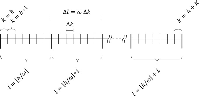
We finally remark that, to avoid too frequent and unpractical changes in the strategies, the control actions can be kept constant over a given period equal to (i.e., for ω time slots). For instance, if Δk is one day, it could be meaningful to set the periodicity of the control actions to one week (i.e., ). Assuming that with the following additional constraints on the control actions are then introduced:
| (36) |
In Fig. 3 we show the different time intervals used to update the state model and the control actions.
Fig. 3.
Scheme adopted for state model and control action time intervals.
3.2. Control multiple objectives
The proposed MPC approach aims at simultaneously optimizing the objectives of all the regions. Thus, the objective function of the overall online optimization problem is formulated as the summation of the single-region objective functions. In turn, the objective function related to region i - denoted as Ji () - is composed by multiple cost terms as follows:
| (37) |
where vectors S i, I i, R i, Q i, T i, H i, E i collect the predicted values of compartment members in region i over the control horizon (e.g., ). Note that coefficients C T, and have a twofold function: on the one hand, they provide a prioritization among the multiple cost terms in (37); on the other hand, they ensure that these terms are homogeneous (namely, they make the three terms dimensionless).
More in detail, the first term in (37) - weighted by coefficient C T - represents the cost incurred by the healthcare system of region i, which is consequent to the predicted epidemic evolution over the whole control horizon. By properly assigning a very large value to C T, we ensure that the number of Threatened individuals Ti(k) related to region i is lower than a prefixed maximum for each time slot k.
The second term in (37) - weighted by coefficient - is the cost incurred by the regional economic system, as a result of applying the intra-region activity restriction in region i over the entire control horizon. It assumes that there is a linear correlation between the level of restriction imposed to the internal activities and the loss of the regional economic productivity.
The third term in (37) - weighted by coefficient - represents the cost incurred by the regional economic system, as a result of regulating the closure of boundaries to region i over the entire control horizon. It assumes that there is a linear correlation between the level of restriction applied to the in- and out-bound mobility and the loss of the regional economic productivity, according to (30).
Summing up, the objective function defined in (37) allows finding a control policy that minimizes the economic loss –quantified through the last two terms of (37)– and simultaneously keeps the number of Threatened under a safety threshold –thanks to the presence of the first term of (37).
Finally, note that weighting coefficients and are region-dependent: this ensures that regional policy makers can adjust these coefficient in accordance with the importance and priority that can be assigned to the above mentioned costs in each region depending on local scenarios, according to (31).
3.3. The proposed multi-region optimal control problem
Having defined the state model, the control variables with the corresponding constraint set, and the objective function related to the online optimization, the optimal control problem is formulated as follows:
| (38) |
The optimization problem (38) has 2MK integer and 7MK real decision variables (i.e., u, r and respectively); furthermore, it presents non-linearities both in the objective function and state model. Consequently, the optimization problem (38) is a mixed-integer non-linear programming (MINLP) problem.
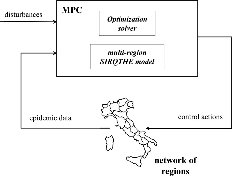
Due to (36), the optimization problem (38) is iteratively solved every ω time slots in accordance with the receding horizon paradigm (see Fig. 3), based on the most recent input data. Only the results referring to the first ω time slots are applied to the system as the optimal control signals, whilst the horizon is shifted ahead. Then, for the next group of ω time slots, a new optimization problem is solved using the updated information on forecasts and system states. This results in the closed-loop control scheme shown in Fig. 4 .
Fig. 4.
The proposed framework of MPC integrating the multi-region SIRQTHE model.
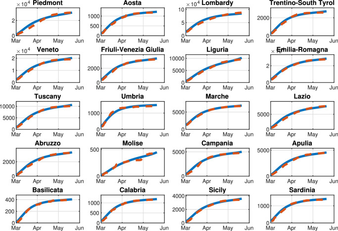
Note that the presented closed-loop feedback control technique may rely both on directly measurable and not directly measurable quantities. In fact, since not all SIRQTHE classes may be directly estimable, at each time shift a procedure for the identification of the model parameters should be conducted. More in detail, at each time shift, the latest data related to the available classes should be used to update the remaining SIRQTHE parameters by employing the dynamical identification procedure (e.g., referring to the Italian scenario, see the identification description defined in Appendix A).
The MPC integrates both the control actions and multi-region epidemic models (described in the previous sections), taking into account the mutual interaction between the effects of the intra-region activity and the inter-region mobility restrictions and the multi-region epidemic dynamics. The MPC law is defined in accordance with an output-feedback formulation. The optimization problem aims at determining the control actions (e.g., intra-region activity restrictions and the inter-region mobility restrictions) for each region, whilst the measured responses coincide with the main epidemic parameters (e.g., number of hospitalized or Quarantined, level of mobility, etc.) monitored by the regional government agencies. Obviously, the estimation of all the variables influencing the epidemic dynamics in the network of regions (i.e., the variables that are not monitored by sensors), as well as the presence of disturbances, can affect the accuracy of the model response. The application of the MPC strategy allows limiting the effects of such uncertainties thanks to the computation of feedback control actions that are based on periodical updates of the actual system state and on the prediction of its evolution in a rolling horizon approach.
4. Numerical experiments on the Italian scenario
In order to validate the optimal control approach of the COVID-19 outbreak, we test the proposed multi-region methodology on the Italian scenario. In particular, in this section we report and analyze the results of the optimal mitigation strategies on the network of Italian regions, i.e., the second level administrative body in Italy. In effect, the Italian scenario suits well the proposed control approach due to two main aspects. On the one hand, the Italian national healthcare system is regionally based. In fact, all the regions have a different level of quality for the healthcare facilities; in addition, each region has different regulations and policies regarding swabs, hospitalization, treatment, and prevention. On the other hand, the spread of COVID-19, and the consequently adopted containment measures, produced extremely heterogeneous effects on the Italian regions: while the North of Italy, and particularly Lombardy, has been facing a tremendous amount of COVID-19 cases (with about one hundred thousand of confirmed cases and sixteen thousand of confirmed deaths as of August 13, 2020 Italian Civil Protection Department, 2020b), the South of Italy is experiencing a relatively stable situation.
First, based on the real data available for the Italian pandemic (see Italian Civil Protection Department, 2020a), we estimate the model parameters for both the single-region and the multi-region SIRQTHE model. Then, we discuss the long-term outcomes that can be achieved by applying the proposed optimal control approach for different restriction policies. We also provide a comparison with respect to the results obtained with three performance evaluation benchmarks, that is: (1) the minimization of the economic cost; (2) the minimization of the Threatened; (3) the threshold rule-based feedback control scheme inspired by the Italian government’s existing protocol (Gazzetta Ufficiale Repubblica Italiana, 2020).
4.1. Definition and set-up of test scenarios
This section reports the main results of the identification to be used as initial conditions for the considered control schemes. The detailed description of the fitting procedure is reported in Appendix A.
The time slot Δk is set to one day, whilst the simulation period is one year. Moreover, since a daily application of the restrictive measures would be unrealistic and impossible to be implemented in real-life, we assume that the control actions are implemented on a weekly basis (i.e., with ).
The initial number of Quarantined, Threatened, Recovered, and Extinct individuals are set to the values of August 13, 2020, according to the real data in Italian Civil Protection Department (2020a). Consequently, the corresponding number of Susceptible, Infected, and Removed individuals is estimated according to the identification procedure reported in Appendix A for the considered date.
We highlight that, since the aim of our work is to reduce the infection rate β(k) so as to contain the number of Threatened people under a well-defined maximum level we assume that β(k) is a function of the mobility level, computed on the basis of the daily Google mobility reports (Google, 2020). Note that is specifically defined for each region, due to the high heterogeneity of the Italian healthcare system. Moreover, we assume that parameters γ, δ, θ, λ, and μ are constant over the prediction horizon and are computed by means of the identification procedure described in Appendix A. Parameters π(k) and ε(k) are time-dependent; however, in the simulations, we set their value to the last fitted value. This hypothesis is reasonable because, although these two parameters are highly variable during the first stage of the pandemic, for long-time observations they settle to a stable value, as shown in Appendix A. Finally, the time-varying migration coefficients ξ i,j(k) () are adapted from Della Rossa et al. (2020).
The optimal control problem (38) is implemented in the Matlab environment (MATLAB, 2020) using the Global Optimization toolbox on a laptop equipped with a 1.3 GHz Intel Core i5 CPU and 8 GB RAM. Since problem (38) falls into the class of MINLP problems, its resolution is non trivial due both to its combinatorial complexity and non-linearity. Therefore, a two-step genetic algorithm approach is here applied for the resolution of (38). In the first phase, being n the number of control variables, we perform 1, 000 n parallel computations of the genetic algorithm with 1, 000 n generations, i.e., an initial population size of 1, 000 n. In the second phase, the outcomes of the first phase are used as the initial population of an additional genetic optimization process.
As for the objective function of (38), the cost coefficients and are set for each region based on the corresponding per capita regional Gross Domestic Product (GDP) normalized by the per capita national GDP (see Appendix B). The coefficient C T is much bigger than and i.e., it is considered equal to 10,000. In fact, we assume that C T is much higher than the other coefficients because our objective is to keep the number of Threatened cases below a maximum level i.e., the first term represents a soft constraint. We do not impose such a condition by means of an explicit additional constraint because, with some settings for the model (e.g., a high infection rate), the problem may become infeasible. Note that, on the basis of the Italian data (Italian Civil Protection Department, 2020b), we set equal to three times the number of Intensive Care Units (ICUs), reported in Appendix B.
Finally, we assume that three different intra-region activity restrictions can be implemented by each region at each time k: lockdown (i.e., ), partial lockdown corresponding to the closure of specific activities, such as universities and schools (i.e., ), or no action (i.e., ). Hence, we have: (). As for the inter-region travel restriction, an on-off strategy can be implemented by each region at each time k: open borders (i.e., ) and closed borders (i.e., ). Hence, we have: ().
4.2. The proposed multi-region control approach: results and discussion
In this section we show the results obtained by the proposed MPC over the given simulation period of one year using a prediction horizon of eight weeks (i.e., ) with the application of the following restriction policies:
-
•
U-U policy : Uniform intra-region activity restrictions and Uniform inter-region travel restrictions.
-
•
D-U policy: Differentiated intra-region activity restrictions and Uniform inter-region travel restrictions.
-
•
D-D policy: Differentiated intra-region activity restrictions and Differentiated inter-region travel restrictions.
As a first outcome, we analyze all the considered restriction policies using several sets of weights by changing the relative importance of intra-region activities with respect to inter-region mobility (that is, by varying parameter α in ).
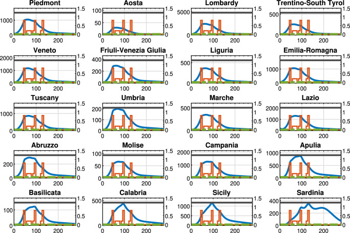
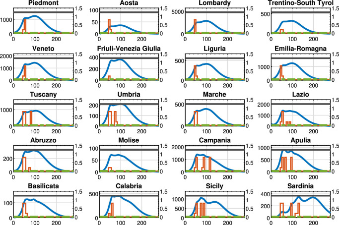
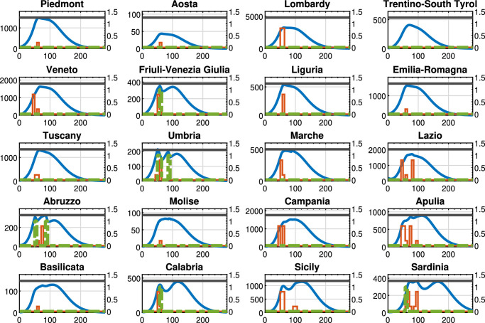
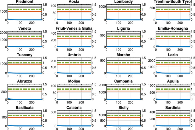
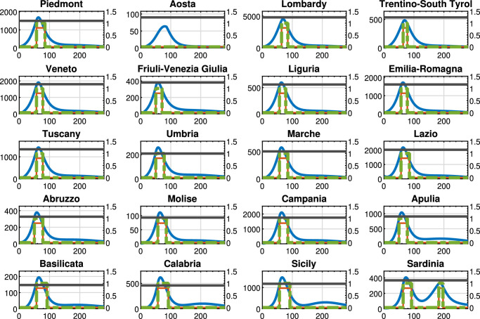
Figures 5 , 6 , 7 show the results obtained for the three above policies when . The blue line represents the time evolution of the Threatened cases, the red line represents the time evolution of the intra-region control actions, and the green dotted line represents the time evolution of the inter-region travel restrictions, while the black line represents the maximum number of Threatened cases that can be treated by the i-th region (i.e., ).
Fig. 5.
Policy U-U, : Threatened cases (blue line), intra-region activity (red line) and inter-region travel (green dotted line) restrictions, the maximum number of Threatened cases that can be treated by the region (black line). For each region, the x-axis reports the time in days, the left y-axis represents the number of Threatened individuals, and the right y-axis represents the value of the control actions.
Fig. 6.
Policy D-U, : Threatened cases (blue line), intra-region activity (red line) and inter-region travel (green dotted line) restrictions, the maximum number of Threatened cases that can be treated by the region (black line). For each region, the x-axis reports the time in days, the left y-axis represents the number of Threatened individuals, and the right y-axis represents the value of the control actions.
Fig. 7.
Policy D-D, : Threatened cases (blue line), intra-region activity (red line) and inter-region travel (green dotted line) restrictions, the maximum number of Threatened cases that can be treated by the region (black line). For each region, the x-axis reports the time in days, the left y-axis represents the number of Threatened individuals, and the right y-axis represents the value of the control actions.
In particular, Fig. 5 highlights that, by adopting the U-U policy, the trend of the control actions is the same for all regions, while the time evolution of the Threatened cases largely varies depending on the considered region. Note that such a policy seems to be unnecessary in some regions, such as Aosta and Trentino-South Tyrol that present a very small amount of Threatened cases with respect to the remaining regions. We highlight that with this policy only the intra-region control policy are applied. Finally, the overall optimal value of the objective function in problem (38) is equal to 462.85.
Figure 6 (D-U policy, with ) shows that the trend of the control actions differs from region to region and the time evolution of the Threatened cases still largely varies depending on the considered region. It has to be noticed that, similarly to Policy U-U, Policy D-U imposes that the regional borders must be open during the observing period. On the contrary, differently from Policy U-U, the intra-region control actions are set coherently to the specific pandemic evolution occurring in each region. In fact, in Aosta no unnecessary restrictions are applied on the intra-region activities. It is also important to remark that the overall optimal value of the objective function in problem (38) is equal to 191.31, that is, about 60% lower than in the Policy U-U, thanks to the differentiated and coherent intra-region control actions.
Moreover, Fig. 7 (D-D policy, with ) shows that the control actions vary from region to region as well as the time evolution of the Threatened cases, but the trend now differs from the previous policies because also the inter-regional control actions are applied. In this case, both intra-region and inter-region control actions are coherently applied depending on the specific pandemic evolution occurring in each region and depending on its economic framework. It is also important to remark that the overall optimal value of the objective function in problem (38) is equal to 171.70, which is the lowest value among the considered policies. In effect, the differentiated intra- and inter-region control actions are coherently set, thus leading to the minimum objective function value for the regional healthcare and economic system.
However, we remark that the emerged finding is an expected outcome. Indeed, the D-D policy presents the least restricted control action set with respect to the D-U and U-U policies, thus leading to a global objective function value that is lower than or equal to that of the other policies (i.e., from a global perspective, the D-D policy generally outperforms the other two policies). Nevertheless, since the objective function (37) is composed by the weighted summation of multiple terms, this conclusion is no more valid when analyzing and comparing the single contributions of the objective function for the three policies. Consequently, the various policies have to be evaluated using further performance indicators different from the composite objective function value, such as the average number of Threatened people and the duration of the control actions. Such a comparative analysis is indeed very useful to policy-makers in supporting the choice of the most suitable strategy to be implemented. As matter of fact, the selection of the best performing policy (i.e., the D-D) is not so obvious due to various contributing reasons related to the complexity of the decision making context. As a consequence, quantifying the gap between the best performing policy and the others and comparing the different policies from various individual points of view actually can help the policy-makers in deeply analyzing and choosing the most effective action by taking into account the different restrictions that could be implemented in a country or a region.
Therefore, in order to effectively evaluate the different control policies, in Tables 1 , 2 , 3 we analyze the results obtained under different values of parameter α ∈ {0.5, 1, 2} in terms of following evaluation indices:
-
•
the average number of Threatened individuals over the control horizon for all the regions and the whole Italy;
-
•
the duration of the lockdown (measured in days) for all the regions;
-
•
the duration of the partial lockdown (measured in days) for all the regions;
-
•
the total number of control action switches, both for intra- and inter-region control actions;
-
•
the duration of the border closure (measured in days) for all the regions;
-
•
the overall cost of the policies over the control horizon for all the regions and the whole Italy.
Table 1.
Comparison of the three simulated policies over 1 year,
| Intra-region control actions | Inter-region control actions | ||||||||||||||||||||
| Region | Average number of Threatened [individuals] | Duration of lockdown [days] | Duration of partial lockdown [days] | Total number of control action switches | Duration of border closure[days] | Total number of control action switches | Global objective function value | ||||||||||||||
| U-U | D-U | D-D | U-U | D-U | D-D | U-U | D-U | D-D | U-U | D-U | D-D | U-U | D-U | D-D | U-U | D-U | D-D | U-U | D-U | D-D | |
| Piedmont | 401 | 551 | 583 | 21 | 7 | 0 | 35 | 7 | 7 | 10 | 3 | 2 | 0 | 0 | 0 | 0 | 0 | 0 | 25.84 | 7.60 | 1.52 |
| Aosta | 11 | 16 | 17 | 21 | 7 | 0 | 35 | 7 | 7 | 10 | 3 | 2 | 0 | 0 | 0 | 0 | 0 | 0 | 31.96 | 9.40 | 1.88 |
| Lombardy | 929 | 1,279 | 1,328 | 21 | 7 | 14 | 35 | 0 | 0 | 10 | 2 | 2 | 0 | 0 | 0 | 0 | 0 | 0 | 31.88 | 7.50 | 15.00 |
| Trentino- South Tyrol | 98 | 141 | 148 | 21 | 0 | 0 | 35 | 14 | 0 | 10 | 2 | 0 | 0 | 0 | 0 | 0 | 0 | 0 | 34.50 | 4.06 | 0.00 |
| Veneto | 447 | 629 | 640 | 21 | 7 | 7 | 35 | 7 | 7 | 10 | 3 | 4 | 0 | 0 | 0 | 0 | 0 | 0 | 27.30 | 8.03 | 8.03 |
| Friuli- V. Giulia | 111 | 158 | 145 | 21 | 0 | 7 | 35 | 7 | 7 | 10 | 2 | 3 | 0 | 0 | 7 | 0 | 0 | 2 | 25.74 | 1.51 | 15.14 |
| Liguria | 140 | 188 | 206 | 21 | 7 | 7 | 35 | 7 | 0 | 10 | 3 | 2 | 0 | 0 | 0 | 0 | 0 | 0 | 26.47 | 7.78 | 6.23 |
| Emilia- Romagna | 409 | 557 | 595 | 21 | 7 | 0 | 35 | 7 | 7 | 10 | 3 | 2 | 0 | 0 | 0 | 0 | 0 | 0 | 29.78 | 8.76 | 1.75 |
| Tuscany | 333 | 431 | 491 | 21 | 21 | 0 | 35 | 0 | 14 | 10 | 4 | 2 | 0 | 0 | 0 | 0 | 0 | 0 | 25.88 | 18.27 | 3.05 |
| Umbria | 78 | 98 | 87 | 21 | 21 | 7 | 35 | 7 | 7 | 10 | 5 | 4 | 0 | 0 | 21 | 0 | 0 | 4 | 20.76 | 15.87 | 24.42 |
| Marche | 136 | 177 | 194 | 21 | 14 | 7 | 35 | 0 | 7 | 10 | 2 | 3 | 0 | 0 | 0 | 0 | 0 | 0 | 23.04 | 10.84 | 6.78 |
| Lazio | 517 | 650 | 692 | 21 | 7 | 14 | 35 | 21 | 7 | 10 | 7 | 6 | 0 | 0 | 0 | 0 | 0 | 0 | 27.56 | 11.35 | 14.59 |
| Abruzzo | 115 | 145 | 136 | 21 | 14 | 7 | 35 | 7 | 7 | 10 | 4 | 4 | 0 | 0 | 14 | 0 | 0 | 4 | 20.99 | 11.11 | 18.52 |
| Molise | 26 | 33 | 35 | 21 | 0 | 0 | 35 | 14 | 7 | 10 | 2 | 2 | 0 | 0 | 0 | 0 | 0 | 0 | 16.95 | 1.99 | 1.00 |
| Campania | 492 | 599 | 640 | 21 | 21 | 14 | 35 | 14 | 0 | 10 | 8 | 4 | 0 | 0 | 0 | 0 | 0 | 0 | 15.26 | 12.56 | 7.18 |
| Apulia | 336 | 398 | 401 | 21 | 21 | 21 | 35 | 7 | 14 | 10 | 7 | 7 | 0 | 0 | 0 | 0 | 0 | 0 | 15.31 | 11.70 | 12.60 |
| Basilicata | 47 | 56 | 58 | 21 | 14 | 0 | 35 | 7 | 7 | 10 | 3 | 2 | 0 | 0 | 0 | 0 | 0 | 0 | 17.95 | 9.50 | 1.06 |
| Calabria | 163 | 208 | 196 | 21 | 7 | 7 | 35 | 7 | 7 | 10 | 4 | 3 | 0 | 0 | 7 | 0 | 0 | 2 | 13.94 | 4.10 | 8.20 |
| Sicily | 425 | 492 | 526 | 21 | 21 | 14 | 35 | 7 | 14 | 10 | 7 | 4 | 0 | 0 | 0 | 0 | 0 | 0 | 14.51 | 11.10 | 8.54 |
| Sardinia | 193 | 199 | 207 | 21 | 28 | 14 | 35 | 14 | 21 | 10 | 7 | 7 | 0 | 0 | 7 | 0 | 0 | 2 | 17.24 | 18.26 | 16.23 |
| Italy | 5407.11 | 7005.38 | 7324.65 | - | - | - | - | - | - | - | - | - | - | - | - | - | - | - | 462.85 | 191.31 | 171.70 |
| Italy Average | - | - | - | 21.00 | 11.55 | 7.00 | 35.00 | 8.05 | 7.35 | 10.00 | 4.05 | 3.25 | 0.00 | 0.00 | 2.80 | 0.00 | 0.00 | 0.70 | - | - | - |
Table 2.
Comparison of the three simulated policies over 1 year,
| Intra-region control actions | Inter-region control actions | ||||||||||||||||||||
| Region | Average number of Threatened [individuals] | Duration of lockdown [days] | Duration of partial lockdown [days] | Total number of control action switches | Duration of border closure [days] | Total number of control action switches | Global objective function value | ||||||||||||||
| U-U | D-U | D-D | U-U | D-U | D-D | U-U | D-U | D-D | U-U | D-U | D-D | U-U | D-U | D-D | U-U | D-U | D-D | U-U | D-U | D-D | |
| Piedmont | 401 | 551 | 578 | 21 | 7 | 7 | 35 | 7 | 0 | 10 | 3 | 2 | 0 | 0 | 0 | 0 | 0 | 0 | 25.84 | 7.60 | 6.08 |
| Aosta | 11 | 16 | 17 | 21 | 7 | 0 | 35 | 7 | 0 | 10 | 3 | 0 | 0 | 0 | 0 | 0 | 0 | 0 | 31.96 | 9.40 | 0.00 |
| Lombardy | 929 | 1,279 | 1,337 | 21 | 7 | 7 | 35 | 0 | 7 | 10 | 2 | 4 | 0 | 0 | 0 | 0 | 0 | 0 | 31.88 | 7.50 | 9.38 |
| Trentino- South Tyrol | 98 | 141 | 151 | 21 | 0 | 0 | 35 | 14 | 0 | 10 | 2 | 0 | 0 | 0 | 0 | 0 | 0 | 0 | 34.50 | 4.06 | 0.00 |
| Veneto | 447 | 629 | 666 | 21 | 7 | 0 | 35 | 7 | 14 | 10 | 3 | 2 | 0 | 0 | 0 | 0 | 0 | 0 | 27.30 | 8.03 | 3.21 |
| Friuli- V. Giulia | 111 | 158 | 150 | 21 | 0 | 0 | 35 | 7 | 14 | 10 | 2 | 4 | 0 | 0 | 7 | 0 | 0 | 2 | 25.74 | 1.51 | 6.81 |
| Liguria | 140 | 188 | 202 | 21 | 7 | 7 | 35 | 7 | 0 | 10 | 3 | 2 | 0 | 0 | 0 | 0 | 0 | 0 | 26.47 | 7.78 | 6.23 |
| Emilia- Romagna | 409 | 557 | 590 | 21 | 7 | 7 | 35 | 7 | 0 | 10 | 3 | 2 | 0 | 0 | 0 | 0 | 0 | 0 | 29.78 | 8.76 | 7.01 |
| Tuscany | 333 | 431 | 478 | 21 | 21 | 7 | 35 | 0 | 0 | 10 | 4 | 2 | 0 | 0 | 0 | 0 | 0 | 0 | 25.88 | 18.27 | 6.09 |
| Umbria | 78 | 98 | 91 | 21 | 21 | 0 | 35 | 7 | 0 | 10 | 5 | 0 | 0 | 0 | 14 | 0 | 0 | 4 | 20.76 | 15.87 | 6.10 |
| Marche | 136 | 177 | 193 | 21 | 14 | 0 | 35 | 0 | 7 | 10 | 2 | 2 | 0 | 0 | 0 | 0 | 0 | 0 | 23.04 | 10.84 | 1.36 |
| Lazio | 517 | 650 | 665 | 21 | 7 | 21 | 35 | 21 | 7 | 10 | 7 | 3 | 0 | 0 | 0 | 0 | 0 | 0 | 27.56 | 11.35 | 21.07 |
| Abruzzo | 115 | 145 | 138 | 21 | 14 | 7 | 35 | 7 | 0 | 10 | 4 | 2 | 0 | 0 | 7 | 0 | 0 | 2 | 20.99 | 11.11 | 8.03 |
| Molise | 26 | 33 | 34 | 21 | 0 | 0 | 35 | 14 | 0 | 10 | 2 | 0 | 0 | 0 | 0 | 0 | 0 | 0 | 16.95 | 1.99 | 0.00 |
| Campania | 492 | 599 | 630 | 21 | 21 | 14 | 35 | 14 | 0 | 10 | 8 | 4 | 0 | 0 | 0 | 0 | 0 | 0 | 15.26 | 12.56 | 7.18 |
| Apulia | 336 | 398 | 402 | 21 | 21 | 21 | 35 | 7 | 0 | 10 | 7 | 4 | 0 | 0 | 0 | 0 | 0 | 0 | 15.31 | 11.70 | 10.80 |
| Basilicata | 47 | 56 | 58 | 21 | 14 | 0 | 35 | 7 | 0 | 10 | 3 | 0 | 0 | 0 | 0 | 0 | 0 | 0 | 17.95 | 9.50 | 0.00 |
| Calabria | 163 | 208 | 205 | 21 | 7 | 14 | 35 | 7 | 0 | 10 | 4 | 4 | 0 | 0 | 0 | 0 | 0 | 0 | 13.94 | 4.10 | 6.56 |
| Sicily | 425 | 492 | 534 | 21 | 21 | 14 | 35 | 7 | 7 | 10 | 7 | 6 | 0 | 0 | 0 | 0 | 0 | 0 | 14.51 | 11.10 | 7.68 |
| Sardinia | 193 | 199 | 203 | 21 | 28 | 14 | 35 | 14 | 28 | 10 | 7 | 7 | 0 | 0 | 0 | 0 | 0 | 0 | 17.24 | 18.26 | 12.17 |
| Italy | 5407.11 | 7005.38 | 7319.54 | - | - | - | - | - | - | - | - | - | - | - | - | - | - | - | 462.85 | 191.31 | 125.76 |
| Italy Average | - | - | - | 21.00 | 11.55 | 7.00 | 35.00 | 8.05 | 4.20 | 10.00 | 4.05 | 2.50 | 0.00 | 0.00 | 1.40 | 0.00 | 0.00 | 0.40 | - | - | - |
Table 3.
Comparison of the three simulated policies over 1 year,
| Intra-region control actions | Inter-region control actions | ||||||||||||||||||||
| Region | Average number of Threatened [individuals] | Duration of lockdown [days] | Duration of partial lockdown [days] | Total number of control action switches | Duration of border closure [days] | Total number of control action switches | Global objective function value | ||||||||||||||
| U-U | D-U | D-D | U-U | D-U | D-D | U-U | D-U | D-D | U-U | D-U | D-D | U-U | D-U | D-D | U-U | D-U | D-D | U-U | D-U | D-D | |
| Piedmont | 401 | 551 | 554 | 21 | 7 | 7 | 35 | 7 | 0 | 10 | 3 | 2 | 0 | 0 | 0 | 0 | 0 | 0 | 25.84 | 7.60 | 6.08 |
| Aosta | 11 | 16 | 16 | 21 | 7 | 0 | 35 | 7 | 0 | 10 | 3 | 0 | 0 | 0 | 0 | 0 | 0 | 0 | 31.96 | 9.40 | 0.00 |
| Lombardy | 929 | 1,279 | 1,265 | 21 | 7 | 14 | 35 | 0 | 7 | 10 | 2 | 3 | 0 | 0 | 0 | 0 | 0 | 0 | 31.88 | 7.50 | 16.88 |
| Trentino- South Tyrol | 98 | 141 | 144 | 21 | 0 | 0 | 35 | 14 | 0 | 10 | 2 | 0 | 0 | 0 | 0 | 0 | 0 | 0 | 34.50 | 4.06 | 0.00 |
| Veneto | 447 | 629 | 617 | 21 | 7 | 7 | 35 | 7 | 7 | 10 | 3 | 3 | 0 | 0 | 0 | 0 | 0 | 0 | 27.30 | 8.03 | 8.03 |
| Friuli- V. Giulia | 111 | 158 | 152 | 21 | 0 | 7 | 35 | 7 | 14 | 10 | 2 | 4 | 0 | 0 | 0 | 0 | 0 | 0 | 25.74 | 1.51 | 9.08 |
| Liguria | 140 | 188 | 199 | 21 | 7 | 0 | 35 | 7 | 0 | 10 | 3 | 0 | 0 | 0 | 0 | 0 | 0 | 0 | 26.47 | 7.78 | 0.00 |
| Emilia- Romagna | 409 | 557 | 572 | 21 | 7 | 7 | 35 | 7 | 0 | 10 | 3 | 2 | 0 | 0 | 0 | 0 | 0 | 0 | 29.78 | 8.76 | 7.01 |
| Tuscany | 333 | 431 | 470 | 21 | 21 | 7 | 35 | 0 | 0 | 10 | 4 | 2 | 0 | 0 | 0 | 0 | 0 | 0 | 25.88 | 18.27 | 6.09 |
| Umbria | 78 | 98 | 89 | 21 | 21 | 7 | 35 | 7 | 0 | 10 | 5 | 2 | 0 | 0 | 14 | 0 | 0 | 4 | 20.76 | 15.87 | 29.30 |
| Marche | 136 | 177 | 174 | 21 | 14 | 7 | 35 | 0 | 0 | 10 | 2 | 2 | 0 | 0 | 7 | 0 | 0 | 2 | 23.04 | 10.84 | 18.98 |
| Lazio | 517 | 650 | 689 | 21 | 7 | 14 | 35 | 21 | 7 | 10 | 7 | 4 | 0 | 0 | 0 | 0 | 0 | 0 | 27.56 | 11.35 | 14.59 |
| Abruzzo | 115 | 145 | 139 | 21 | 14 | 0 | 35 | 7 | 14 | 10 | 4 | 4 | 0 | 0 | 7 | 0 | 0 | 2 | 20.99 | 11.11 | 14.82 |
| Molise | 26 | 33 | 35 | 21 | 0 | 0 | 35 | 14 | 0 | 10 | 2 | 0 | 0 | 0 | 0 | 0 | 0 | 0 | 16.95 | 1.99 | 0.00 |
| Campania | 492 | 599 | 642 | 21 | 21 | 14 | 35 | 14 | 0 | 10 | 8 | 4 | 0 | 0 | 0 | 0 | 0 | 0 | 15.26 | 12.56 | 7.18 |
| Apulia | 336 | 398 | 398 | 21 | 21 | 21 | 35 | 7 | 7 | 10 | 7 | 4 | 0 | 0 | 0 | 0 | 0 | 0 | 15.31 | 11.70 | 11.70 |
| Basilicata | 47 | 56 | 58 | 21 | 14 | 0 | 35 | 7 | 0 | 10 | 3 | 0 | 0 | 0 | 0 | 0 | 0 | 0 | 17.95 | 9.50 | 0.00 |
| Calabria | 163 | 208 | 210 | 21 | 7 | 7 | 35 | 7 | 14 | 10 | 4 | 5 | 0 | 0 | 0 | 0 | 0 | 0 | 13.94 | 4.10 | 4.92 |
| Sicily | 425 | 492 | 528 | 21 | 21 | 14 | 35 | 7 | 14 | 10 | 7 | 6 | 0 | 0 | 0 | 0 | 0 | 0 | 14.51 | 11.10 | 8.54 |
| Sardinia | 193 | 199 | 203 | 21 | 28 | 14 | 35 | 14 | 28 | 10 | 7 | 9 | 0 | 0 | 0 | 0 | 0 | 0 | 17.24 | 18.26 | 12.17 |
| Italy | 5407.11 | 7005.38 | 7151.51 | - | - | - | - | - | - | - | - | - | - | - | - | - | - | - | 462.85 | 191.31 | 175.37 |
| Italy Average | - | - | - | 21.00 | 11.55 | 7.35 | 35.00 | 8.05 | 5.60 | 10.00 | 4.05 | 2.80 | 0.00 | 0.00 | 1.40 | 0.00 | 0.00 | 0.40 | - | - | - |
By analyzing Table 1, it can be observed that, if a similar importance weight is assigned to both the intra- and inter-region actions (i.e., for ), then the average number of Threatened people assumes the lowest value with the U-U policy, thus making it preferable from a social perspective, whereas the average duration of the lockdown is the highest with the lowest number of control actions switches. Similar findings arise when analyzing Tables 2 and 3, which respectively refer to inter-region actions that are twice (i.e., ) and half (i.e., ) important than intra-region ones. As a result, we can conclude that, although the D-D policy, thanks to differentiated actions on intra-region activity and inter-region mobility restrictions, ensures the lowest global objective function value, it does not guarantee the lowest number of Threatened cases.
4.3. A comparison with benchmark control strategies
In this section, we introduce some reference strategies to compare the examining the effectiveness of the proposed optimal control approach. In particular, three simple benchmark strategies are defined:
-
•
Benchmark control strategy 1: No restrictions are applied for the whole simulation period, ignoring the impact on the healthcare system.
-
•
Benchmark control strategy 2: All restrictions are applied for the whole simulation period, i.e., all the intra-region and inter-region restrictions are used at their maximum value to control and flatten the number of cases, ignoring any economic impact.
-
•
Benchmark control strategy 3: At the beginning of each week, all restrictions are applied in a single region if the number of Threatened is higher than a safety threshold.
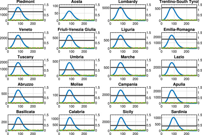
Note that the first two strategies represent two ideal extreme cases, since they correspond to take only the economic or the health perspective into account, respectively. Instead, the third strategy is a simple but at the same time realistic feedback control strategy to mitigate the COVID-19 outbreak. Figures 8 , 9 , 10 show the results obtained for the three benchmark control strategies. The blue line represents the time evolution of the Threatened cases, the red line represents the time evolution of the intra-region control actions, and the green dotted line represents the time evolution of the inter-region travel restrictions, while the black line represents the maximum number of Threatened cases that can be treated by the i-th region (i.e., ).
Fig. 8.
Benchmark control strategy 1: Threatened cases (blue line), intra-region activity (red line) and inter-region travel (green dotted line) restrictions, and the maximum number of Threatened that can be treated by the region (black line). For each region, the x-axis reports the time in days, the left y-axis represents the number of Threatened, and the right y-axis represents the value of the control actions.
Fig. 9.
Benchmark control strategy 2: Threatened cases (blue line), intra-region activity (red line) and inter-region travel (green dotted line) restrictions, and the maximum number of Threatened that can be treated by the region (black line). For each region, the x-axis reports the time in days, the left y-axis represents the number of Threatened, and the right y-axis represents the value of the control actions.
Fig. 10.
Benchmark control strategy 3: Threatened cases (blue line), intra-region activity (red line) and inter-region travel (green dotted line) restrictions, and the maximum number of Threatened that can be treated by the region (black line). For each region, the x-axis reports the time in days, the left y-axis represents the number of Threatened, and the right y-axis represents the value of the control actions.
In Fig. 8 we show the results of benchmark control strategy 1, i.e., the case where no restrictions are applied and the control actions at each week are null ( and for each region i for each time k). The reported graph highlights that with the current model parameters, applying no control actions would result in an overload of the national healthcare system in almost all Italian regions. At the same time, this solution corresponds to the minimization of only the last two terms of (37), i.e., only the economic part.
Conversely, in Fig. 9 we show the results of benchmark control strategy 2, i.e., the case where all the restrictions are applied at their maximum value ( and for each region i at each time k of the simulation period). In this case the number of Infected falls to zero; however, the economic cost is the highest (i.e., 19603.17).
Finally, in Fig. 10, we show the results of benchmark control strategy 3. In this approach, the control actions are applied when the number of Threatened cases is higher than a predetermined threshold. More in detail, at the end of each week, if the Threatened cases are higher than the threshold level, all the measures (intra and inter-region control actions) are applied in the subsequent week. This strategy is similar to the protocol implemented by the Italian government (Gazzetta Ufficiale Repubblica Italiana, 2020). In fact, the current Italian protocol considers safety thresholds on the number of infected and Threatened. When these thresholds are exceeded in a specific region, the restrictive measures are applied to reduce the number of cases. The threshold directly influences the total economic cost and the number of Threatened people. In fact, a high threshold leads to a large number of Threatened cases that may exceed the maximum capacity. Conversely, a low threshold would keep the number of cases low by having a higher economic cost. In our simulation, we assume a safety level for all the regions equal to ; this results in an economic cost of 830.33., i.e., only the last two terms of (37). Moreover, the figure shows that this strategy is ineffective in containing the number of Threatened cases.
We now compare the results of the MPC approach (Section 4.2) with respect to the above results. Disregarding the difference between the three different policies (i.e., U-U, D-U, and D-D), the objective function value is always significantly lower than that of all the benchmark control strategies, due to different factors as detailed in the sequel.
Comparing the proposed MPC results with the benchmark control strategy 1, it is apparent that, since no restrictions are applied, the number of Threatened largely exceeds the maximum limit in all the regions in the latter case. Hence, although the economic cost is null, the global objective function value is much higher than that of the proposed MPC approach.
Referring to the benchmark control strategy 2, the number of Threatened is kept at the lowest value. Nevertheless, since the economic aspect is ignored, the last two parts of the objective function largely arise, thus leading to a higher global objective function value with respect to that of the presented MPC method.
The comparison between the proposed MPC and the benchmark control strategy 3 is of particular interest. The latter shows an economic cost, which is computed by taking into account only the last two parts of the objective function, four times higher than that of the D-D policy and two times higher than that of the U-U one. In addition, since the benchmark strategy 3 is unable to keep the number of Threatened below the maximum limit in all the regions, the first part of the objective function makes the total cost much higher than the proposed MPC approach.
Summing up, from the above simulations it arises that the proposed optimal control approach provides the best compromise between the two most important governmental aspects (that is, the economic and the social features of interventions), being able to keep the number of Threatened cases below a maximum limit while minimizing the economic cost of the eventually required lockdown periods. Consequently, the proposed methodology represents a useful support tool for policy-makers to mitigate the COVID-19 outbreak in case of secondary pandemic waves.
5. Conclusions and future works
In this paper, we propose a novel feedback control strategy aimed at supporting policy-makers in efficiently mitigating the effects of COVID-19 pandemic contagions in multi-region areas, such as Italy, where the contagion peak has been reached and, in a post-lockdown phase, coordinated regional restarting strategies are needed.
The presented methodology makes joint use of an epidemiological SIR-based model (namely a SIRQTHE model) in conjunction with a non-linear Model Predictive Control (MPC) approach, with the final aim of minimizing the cost of the adopted mitigation strategies, while ensuring that the capacity of the regional healthcare systems is not violated. First, the SIRQTHE model allows to consider seven compartments of individuals (that is, Susceptible,Infected, Removed, Quarantined, Threatened, Healed, and Extinct), thus ensuring a detailed representation of the pandemic dynamics, which is further guaranteed thanks to the definition of time-varying parameters. In addition, the multi-region framework allows to simultaneously take into account both the actions taken at a national level in terms of border activities between the regions and the specific strategies undertaken at each regional level. On the one hand, the proposed approach fills a gap in the existing literature, where in reference to a multi-region scenario there is a lack of investigations on optimal control approaches aimed at effectively coping with possible onset of further epidemic waves, while efficiently returning economic activities to the standard level of intensity. On the other hand, the application to the network of Italian regions based on real data-sets highlights the planning utility and flexibility of the proposed MPC approach in determining differentiated, as well as coordinated, optimal control actions over all the given regions.
An additional merit of the developed approach is in its generalizability to different levels of spatial scale. Whilst in the presented numerical experiments we choose the network of Italian regions as the multi-region area under control, an interesting development of the research can be to apply the MPC approach to determine the differentiated, as well as coordinated, optimal control policies of higher- and lower-granularity networks, such as, for instance, the counties in the European Union or the districts within the same region.
Nonetheless, this study is not without limitations, which still need to be investigated in future works. In particular, the main limitation of the proposed framework relies on the centralized computation of the regional optimal control policies. Due to economical, political, and societal reasons, a centralized control approach may not be appealing in the epidemic control of a multi-region framework. At the same time, since all the regions are coupled by states and inputs, the cooperation between regions should be encouraged to improve the system-wide performance through the avoidance of uncoordinated behavior of individual regions. Hence, the optimization of the regional strategies may be preferably performed through a cooperative distributed framework. Therefore, our future work will mainly be devoted to define an iterative mechanism to determine the regional optimal control policies in a cooperative distributed setting.
Finally, one may observe that results and implications are derived from a simple model of control and mitigation actions, since we consider a finite set of intra-region activity and inter-region mobility restrictions producing additive effects on the reduction of infection. Actually, this limitation is only apparent, since the proposed model can be easily generalized to more complex cases by adding other terms in the objective function and constraints to deal with the eventual finer control and mitigation actions producing combined non-linear effects on the analyzed epidemic dynamics.
Declaration of Competing Interest
The authors declare that they have no known competing financial interests or personal relationships that could have appeared to influence the work reported in this paper.
Footnotes
This work received funding from the Italian University and Research Ministry under project RAFAEL (National Research Program, contract No. ARS01_00305).
Appendix A. Parameters identification
In this Appendix we explain how we calibrate the SIRQTHE model for the considered numerical experiments. In fact, the genuineness of any model depends on the number and quality of raw data adopted in the selection of variables to be used and parameters to be calibrated. Therefore, any model should rely as much as possible on the available data and on the prior knowledge of the system to model.
A1. Data availability in the Italian scenario and main assumptions
The Italian State body largely responsible for the management of natural disasters and catastrophes is the Protezione Civile (Italian Civil Protection Department, 2020b) (i.e., the Italian Civil Protection Department) (Italian Civil Protection Department, 2020b). During a pandemic emergency, the Protezione Civile is responsible for collecting and elaborating all the data related with the pandemic.
More in detail, several data (and analyses) on a daily basis are available for the COVID-19 pandemic (Italian Civil Protection Department, 2020a):
-
•
total cases: cumulative number of people infected, also comprehending healed and dead;
-
•
hospitalized in a non-critical situation: number of people that are identified as currently infected and as such they are hospitalized, although their situation is not critical;
-
•
hospitalized in a critical situation: number of people that are currently hospitalized in an Intensive Care Unit because of their severe situation;
-
•
in quarantine: number of people recognized as infected; however, due to their mild or absent symptoms, they are legally obliged to stay in isolation at home;
-
•
healed: number of people recognized as infected, but dismissed because healed;
-
•
deceased: number of people dead because of COVID-19;
-
•
swabs: number of swabs made by the national healthcare system.
Besides the above data, in order to perform a realistic and fruitful selection of the model parameters for the whole Italian outbreak (i.e., from February until to the post-lockdown restarting phase in June) we should not neglect that all parameters are variable and time-dependent, especially during the first spread of the virus in a country.
In the literature, a pragmatic and widely adopted approach to overcome this limitation consists in fitting the model by employing different time windows, which reflect the different stages of the epidemic, and to set the parameters constant within each of these periods (Bin et al., 2020). This leads to an acceptable fitting only when additional information is included in the fitting phase. For instance, it is possible to add constraints on the parameters based on the available scientific knowledge.
Conversely, in this paper, we fit the model by assuming that the required parameters can be predicted with some time-dependent functions. Moreover, the following assumptions are made on the parameters:
-
•βi(k) (i.e., the infection rate of region i at time k): in the related literature (see, e.g., the work in Della Rossa et al. (2020)), this parameter typically ranges between 0.35 and 0.55 in the absence of social distancing policies and people awareness. However, this value highly decreases during lockdown periods. In our work, to perform a continuous fitting of the COVID-19 from March to June (that is, during the post-lockdown phase), we correlate the evolution of β with the evolution of people’s mobility computed on the basis of the daily Google mobility reports (Google, 2020), aggregated on a weekly basis. Therefore, the infection rate at the week w is defined as:
where is the infection rate in region i when no containment measures are applied, Mi( · ) is the weekly mobility level (i.e., Mi( · ) is a function of weeks and it ranges between 0 and 1) in region i, and di is the delay of effects that mobility has on the contagion in region i. Note that, since the effects of social restrictions are not immediate, after a sensitivity analysis on the available data we consider a delay of one week in all the regions. Hence, we set . Also note that the use of a different for each region would help the model fitting model, since is likely to increase in the regions with a higher population density (we refer the interested reader to the work in Hu, Nigmatulina, & Eckhoff (2013)). Nevertheless, for the sake of limiting the number of parameters, we set for all the Italian regions a uniform value for this parameter: .(A.1) -
•
γ and δ (i.e., the rate of healing of unrecognized infected people who do not need hospitalization and the rate of healing of Quarantined people who do not need hospitalization, respectively): the value assigned to these parameters can be approximated by a constant since currently there is no proof that the virus has mutated. In theory, these two parameters have different values: in several countries, someone may leave the quarantine only after two negative swabs, i.e., a person may be forced to be in quarantine even after clinically healed. Nevertheless, for the sake of reducing the model parameters in the identification phase, we assume, without loss of generality, that these two parameters equal. In particular, the literature findings show that setting is appropriate (see, e.g., the work in Bertozzi, Franco, Mohler, Short, & Sledge (2020)) and therefore we assume this value for all the regions.
-
•
θi (i.e., the rate of infected people that are recognized and Quarantined of region i): this parameter is mainly related with the specific policy adopted by each region and the number of laboratory testing capacities (e.g., in terms of tested swabs). However, when the laboratory limits were reached at the beginning of March the number of tested swabs became constant. Therefore, we assume this parameter as time-independent, but variable from region to region.
-
•
λ and μ (i.e., the rate of people recognized only when strong symptomatic conditions occur and the rate of Quarantined people to be hospitalized, respectively): both parameters represent the rates of people that need to be hospitalized. As these parameters are only related with the virus nature, we assume they are both constant and equal for all the regions.
-
•πi(k) (i.e., the recovery rate of region i at time k): this parameter is far from being constant during the spread of COVID-19. The national healthcare system may not be prepared and does not have therapeutic procedures for patients with symptoms that have never been seen before. This means that initially the evolution of the number of recoveries can be slow until a constant value is reached, i.e., when the healthcare system becomes ready and prepared. In particular, on the basis of the performed analyses, we impose the parameter π to be time-dependent with the following formulation for each region:
(A.2) -
•εi(k) (i.e., the death rate of region i at time k): the number of deaths is not constant and hopefully decreases with time. This is mainly due to the availability of new clinical treatments. Furthermore, at the beginning of an epidemic, when the screening of infected people is low, only the sever symptoms cases are recognized and treated. With the ongoing of the pandemic, more cases are recognized as infected, and hence the percentage of severe symptoms cases becomes lower. Therefore, taking into account the performed analyses, we set parameter εi as time-dependent with the following formulation for each region:
(A.3) -
•
ξ i,j(k) (i.e., the inter-region mobility coefficient between regions i and j at time k): these parameters are adapted from Della Rossa et al. (2020) due to the different model assumptions; in detail, the aforementioned work considers the interaction between the people between different regions. In contrast, we consider physical migration between different classes.
A2. Parameters identification for Single-region SIRQTHE models
In order to estimate the parameters for the Single-region SIRQTHE model, we adopt a pragmatic approach with a least-squares optimization technique based on the real data combined with hard constraints to enforce the prior knowledge on the system.
The containment measures of the pandemic in Italy can be divided into two main phases, one following February 23, which mainly concerned Northern Italy, and a second one following March 09, including the more restrictive measures affecting the whole national territory. The first restrictive measures, which comprehend the closure of schools, universities, and bars and restaurants after 6 p.m., had limited effects on the contagion dynamics and, as the crisis worsened, the need for more severe restrictions motivated the second phase, which turned into a total lockdown where all the non-essential production activities were shut down. Therefore, in this phase, the Italian scenario turns into a network of isolated regions, corresponding to the set of M Single-region SIRQTHE models. These models are fitted through the data related to the period when the movements between regions were not permitted in Italy (i.e., from March 15 to May 31). Each regional decoupled model is composed by seven equations and seven parameters, which are reduced to six equations and six parameters since the Removed are calculated in accordance with (4) adapted to the SIRQTHE discrete-time seven-compartments model. Since two of these equations are highly non-linear, the fitting procedure is highly non-convex; indeed, as proposed in Della Rossa et al. (2020), improved results can be obtained by splitting each regional model into two simpler sub-models and thus performing a two-stage fitting procedure.
In the first stage we analyze the following sub-model:
| (A.4) |
| (A.5) |
| (A.6) |
where is the cumulative number of Infected people. It is clear that β 0, and the initial condition are the only parameters to be estimated. The estimation of such parameters consists in minimizing the mean squared error (MSE) of the model with respect to the real data, which is defined as:
| (A.7) |
Figure A.11 reports the real data and the model outputs related to the above introduced class C of Infected people, thus showing the effectiveness of the fitting first stage for all the regions.
Fig. A.11.
Cumulative number of Infected cases for all the Italian regions from March to June 2020: real data (red dashed line) and Single-region SIRQTHE model output (blue line).
In the second stage, we analyze the following sub-model:
| (A.8) |
| (A.9) |
| (A.10) |
| (A.11) |
where we assume that the parameters π(k) and ε(k) are time-dependent.
Figures A.12 and A.13 respectively report the real data and the fitted curve for the parameters π(k) and ε(k), confirming that the inferred formulations in (A.2) and (A.3) well fit the real scenario over all the regions. Finally, Figs. A.14 , A.15 , A.16 , A.17 report the real data and the model outputs related to the classes Q, T, H, and E addressed by the second sub-model, thus showing the effectiveness of the overall fitting procedure.
Fig. A.12.
The healing rate π(k) for all the Italian regions from March to June 2020: real data (red stars) and Single-region SIRQTHE model output (blue line).
Fig. A.13.
The mortality rate ε(k) for all the Italian regions from March to June 2020: real data (red stars) and Single-region SIRQTHE model output (blue line).
Fig. A.14.
Recognized cases for all the Italian regions from March to June 2020: real data (red stars) and Single-region SIRQTHE model output (blue line).
Fig. A.15.
Threatened cases for all the Italian regions from March to June 2020: real data (red stars) and Single-region SIRQTHE model output (blue line).
Fig. A.16.
Healed cases for all the Italian regions from March to June 2020: real data (red stars) and Single-region SIRQTHE model output (blue line).
Fig. A.17.
Deaths for all the Italian regions from March to June 2020: real data (red stars) and Single-region SIRQTHE model output (blue line).
A3. Parameters identification for the multi-region SIRQTHE model
The estimation of the parameters of the Multi-region SIRQTHE model follows a two-stage fitting procedure similar to that described in A.2, except for the differences highlighted in the sequel. First, we note that, since the multi-region model takes the migrations between regions into account, the corresponding fitting window includes also periods when the inter-region borders are opened in Italy (i.e., from February 29 to June 3). Second, instead of individually identifying the parameters of independent single-region sub-models (A.4)-(A.6), we simultaneously fit the parameters of the entire network of regional sub-models coupled by the migration coefficients ξ i,j(k). These coefficients are adapted from Della Rossa et al. (2020): in particular, the authors in Della Rossa et al. (2020) use two sets of average number of people migrated from region i to region j, respectively referred the lockdown and post-lockdown phases; in our model we normalize the data used in Della Rossa et al. (2020) with respect to the regional population in order to determine the migration rate ξ i,j(k) () and we compute ξ i,i(k) () through (19). Finally, the identification of the parameters of sub-model (A.8)-(A.11) is individually performed for each region. Figures A.18 , A.19 , A.20 , A.21 , A.22 show the real data and the model outputs related to the classes C, Q, T, H, and E addressed by the multi-region model. Observing Fig. A.18, Fig. A.19, Fig. A.20, Fig. A.21, Fig. A.22 it is possible to notice that in all regions the state variables computed by the Multi-region SIRQTHE model well fit the real data.
Fig. A.18.
Cumulative number of Infected cases for all the Italian regions from March to June 2020: real data (dashed red line) and Multi-region SIRQTHE model output (blue line).
Fig. A.19.
Recognized cases for all the Italian regions from March to June 2020: real data (dashed red line) and Multi-region SIRQTHE model output (blue line).
Fig. A.20.
Threatened cases for all the Italian regions from March to June 2020: real data (dashed red line) and Multi-region SIRQTHE model output (blue line).
Fig. A.21.
Healed cases for all the Italian regions from March to June 2020: real data (dashed red line) and Multi-region SIRQTHE model output (blue line).
Fig. A.22.
Deaths for all the Italian regions from March to June 2020: real data (dashed red line) and Multi-region SIRQTHE model output (blue line).
Appendix B. List of parameters used in the MPC scheme
In Table B.4 we report the list of parameters used in the MPC scheme for the Italian case study, namely the population (Italian Statistics National Institute, 2020), the number of ICU beds (Italian Ministry of Health, 2020) and the per capita GDP (Italian Statistics National Institute, 2020) for each Italian region.
Table B.4.
Regional and national data used in case study.
| Region | Population (2019) | ICU beds (2020) | Per capita GDP (2018) [M€ ] |
|---|---|---|---|
| Piedmont | 4 356 406 | 499 | 31.49 |
| Aosta | 125 666 | 30 | 38.94 |
| Lombardy | 10 060 574 | 1 600 | 38.84 |
| Trentino-South Tyrol | 1 072 276 | 178 | 42.04 |
| Veneto | 4 905 854 | 600 | 33.27 |
| Friuli-Venezia Giulia | 1 215 220 | 127 | 31.36 |
| Liguria | 1 550 640 | 186 | 32.25 |
| Emilia-Romagna | 4 459 477 | 539 | 36.29 |
| Tuscany | 3 729 641 | 447 | 31.54 |
| Umbria | 882 015 | 70 | 25.29 |
| Marche | 1 525 271 | 168 | 28.08 |
| Lazio | 5 879 082 | 675 | 33.58 |
| Abruzzo | 1 311 580 | 109 | 25.58 |
| Molise | 305 617 | 31 | 20.65 |
| Campania | 5 801 692 | 586 | 18.59 |
| Apulia | 4 029 053 | 302 | 18.65 |
| Basilicata | 562 869 | 49 | 21.87 |
| Calabria | 1 947 131 | 153 | 16.98 |
| Sicily | 4 999 891 | 392 | 17.68 |
| Sardinia | 1 639 591 | 123 | 21.01 |
| Italy | 60 359 546 | 6 864 | 29.22 |
References
- Alleman T., Torfs E., Nopens I. COVID-19: From model prediction to model predictive control. https://biomath. ugent. be/sites/default/files/2020-04/Alleman_etal_v2. pdf, accessed April. 2020;30:2020. [Google Scholar]
- Bai Y., Yao L., Wei T., Tian F., Jin D.-Y., Chen L., Wang M. Presumed asymptomatic carrier transmission of covid-19. Jama. 2020;323(14):1406–1407. doi: 10.1001/jama.2020.2565. [DOI] [PMC free article] [PubMed] [Google Scholar]
- Bertozzi A.L., Franco E., Mohler G., Short M.B., Sledge D. The challenges of modeling and forecasting the spread of covid-19. arXiv preprint arXiv:2004.04741. 2020 doi: 10.1073/pnas.2006520117. [DOI] [PMC free article] [PubMed] [Google Scholar]
- Bin M., Cheung P., Crisostomi E., Ferraro P., Myant C., Parisini T., Shorten R. On fast multi-shot epidemic interventions for post lock-down mitigation: Implications for simple covid-19 models. arXiv preprint arXiv:2003.09930. 2020 [Google Scholar]
- Bin M., Cheung P., Crisostomi E., Ferraro P., Myant C., Parisini T., Shorten R. On fast multi-shot epidemic interventions for post lock-down mitigation: Implications for simple covid-19 models. arXiv preprint arXiv:2003.09930. 2020 [Google Scholar]
- Brugnano L., Iavernaro F., Zanzottera P. Mathematical Methods in the Applied Sciences. Wiley Online Library; 2020. A multiregional extension of the SIR model, with application to the COVID-19 spread in Italy. [DOI] [PMC free article] [PubMed] [Google Scholar]
- Bussell E.H., Dangerfield C.E., Gilligan C.A., Cunniffe N.J. Applying optimal control theory to complex epidemiological models to inform real-world disease management. Philosophical Transactions of the Royal Society B. 2019;374(1776):20180284. doi: 10.1098/rstb.2018.0284. [DOI] [PMC free article] [PubMed] [Google Scholar]
- Calafiore G.C., Novara C., Possieri C. A modified SIR model for the COVID-19 contagion in Italy. arXiv preprint arXiv:2003.14391. 2020 doi: 10.1016/j.arcontrol.2020.10.005. [DOI] [PMC free article] [PubMed] [Google Scholar]
- Carli R., Cavone G., Dotoli M., Epicoco N., Scarabaggio P. 2019 ieee international conference on systems, man and cybernetics (smc) IEEE; 2019. Model predictive control for thermal comfort optimization in building energy management systems; pp. 2608–2613. [Google Scholar]
- Casella F. Can the COVID-19 epidemic be controlled on the basis of daily test reports? IEEE Control Systems Letters. 2021;5(3):1079–1084. [Google Scholar]
- Chen Z. Discrete-time vs. continuous-time epidemic models in networks. IEEE Access. 2019;7:127669–127677. [Google Scholar]
- Della Rossa F., Salzano D., Di Meglio A. Intermittent yet coordinated regional strategies can alleviate the COVID-19 epidemic: A network model of the Italian case. arXiv preprint arXiv:2005.07594. 2020 doi: 10.1038/s41467-020-18827-5. [DOI] [PMC free article] [PubMed] [Google Scholar]
- Di Domenico L., Pullano G., Coletti P., Hens N., Colizza V. Technical Report. Report; 2020. Expected impact of school closure and telework to mitigate COVID-19 epidemic in France. [Google Scholar]
- Ferguson N., Laydon D., Nedjati-Gilani G., Imai N., Ainslie K., Baguelin M.…Cuomo-Dannenburg G. Report 9: Impact of non-pharmaceutical interventions (npis) to reduce covid19 mortality and healthcare demand. Imperial College London. 2020;10:77482. [Google Scholar]
- Gazzetta Ufficiale Repubblica Italiana, Decree of the President of the Council of Ministers april 26, 2020: urgent measures regarding the containment and management of the COVID-19 epidemiological emergency (in Italian), 2020. [Online; accessed 26. Aug. 2020], https://www.gazzettaufficiale.it/eli/id/2020/04/27/20A02352/sg.
- Gatto M., Bertuzzo E., Mari L., Miccoli S., Carraro L., Casagrandi R., Rinaldo A. Spread and dynamics of the covid-19 epidemic in italy: Effects of emergency containment measures. Proceedings of the National Academy of Sciences. 2020;117(19):10484–10491. doi: 10.1073/pnas.2004978117. [DOI] [PMC free article] [PubMed] [Google Scholar]
- Giordano G., Blanchini F., Bruno R., Colaneri P., Di Filippo A., Di Matteo A., Colaneri M. Modelling the COVID-19 epidemic and implementation of population-wide interventions in Italy. Nature Medicine. 2020:1–6. doi: 10.1038/s41591-020-0883-7. [DOI] [PMC free article] [PubMed] [Google Scholar]
- Hernandez-Vargas E.A., Alanis A.Y., Tetteh J. A new view of multiscale stochastic impulsive systems for modeling and control of epidemics. Annual Reviews in Control. 2019;48:242–249. [Google Scholar]
- Hethcote H.W. The mathematics of infectious diseases. SIAM Review. 2000;42:599–653. [Google Scholar]
- Hu H., Nigmatulina K., Eckhoff P. The scaling of contact rates with population density for the infectious disease models. Mathematical biosciences. 2013;244(2):125–134. doi: 10.1016/j.mbs.2013.04.013. [DOI] [PubMed] [Google Scholar]
- Italian Ministry of Health, The Italian Ministry of Health website (2020). http://www.salute.gov.it, Accessed: 2020-08-13.
- Italian Statistics National Institute, The Italian National Institute of Statistics website (2020). [Online: Accessed: 2020-08-13]. https://www.istat.it/en/information-and-services.
- Italian Civil Protection Department, The Civil Protection Department COVID-19 dashboard (2020a). [Accessed: 2020-08-13] http://opendatadpc.maps.arcgis.com/apps/opsdashboard/index.html#/b0c68bce2cce478eaac82fe38d4138b1.
- Italian Civil Protection Department, The Civil Protection Department website, 2020b. http://www.protezionecivile.gov.it/, Accessed: 2020-08-13.
- Köhler J., Schwenkel L., Koch A., Berberich J., Pauli P., Allgöwer F. Robust and optimal predictive control of the COVID-19 outbreak. arXiv preprint arXiv:2005.03580. 2020 doi: 10.1016/j.arcontrol.2020.11.002. [DOI] [PMC free article] [PubMed] [Google Scholar]
- Leung K., Wu J.T., Liu D., Leung G.M. First-wave covid-19 transmissibility and severity in china outside hubei after control measures, and second-wave scenario planning: a modelling impact assessment. The Lancet. 2020 doi: 10.1016/S0140-6736(20)30746-7. [DOI] [PMC free article] [PubMed] [Google Scholar]
- MATLAB . The MathWorks Inc.; Natick, Massachusetts: 2020. Matlab user guide 9.8.0.135996 (R2020a) [Google Scholar]
- Mei W., Mohagheghi S., Zampieri S., Bullo F. On the dynamics of deterministic epidemic propagation over networks. Annual Reviews in Control. 2017;44:116–128. [Google Scholar]
- Morato M.M., Normey-Rico J.E., Sename O. Model predictive control design for linear parameter varying systems: A survey. Annual Reviews in Control. 2020 [Google Scholar]
- Ngonghala C.N., Iboi E., Eikenberry S., Scotch M., MacIntyre C.R., Bonds M.H., Gumel A.B. Mathematical assessment of the impact of non-pharmaceutical interventions on curtailing the 2019 novel coronavirus. Mathematical Biosciences. 2020:108364. doi: 10.1016/j.mbs.2020.108364. [DOI] [PMC free article] [PubMed] [Google Scholar]
- Nowzari C., Preciado V.M., Pappas G.J. Analysis and control of epidemics: A survey of spreading processes on complex networks. IEEE Control Systems Magazine. 2016;36(1):26–46. [Google Scholar]
- Rachah A., Torres D.F. Mathematical modelling, simulation, and optimal control of the 2014 ebola outbreak in west africa. Discrete Dynamics in Nature and Society. 2015;2015 [Google Scholar]
- Ridenhour B., Kowalik J.M., Shay D.K. Unraveling r 0: Considerations for public health applications. American journal of public health. 2018;108(S6):S445–S454. doi: 10.2105/AJPH.2013.301704. [DOI] [PMC free article] [PubMed] [Google Scholar]
- Rodrigues H.S., Monteiro M.T.T., Torres D.F. Vaccination models and optimal control strategies to dengue. Mathematical biosciences. 2014;247:1–12. doi: 10.1016/j.mbs.2013.10.006. [DOI] [PubMed] [Google Scholar]
- Google LLC. Google COVID-19 Community Mobility Reports, (2020). http://www.google.com/covid19/mobility, Accessed: 2020-08-13.
- Sélley F., Besenyei Á., Kiss I.Z., Simon P.L. Dynamic control of modern, network-based epidemic models. SIAM Journal on applied dynamical systems. 2015;14(1):168–187. [Google Scholar]
- Silva C.J., Torres D.F. Optimal control for a tuberculosis model with reinfection and post-exposure interventions. Mathematical Biosciences. 2013;244(2):154–164. doi: 10.1016/j.mbs.2013.05.005. [DOI] [PubMed] [Google Scholar]
- Watkins N.J., Nowzari C., Pappas G.J. Robust economic model predictive control of continuous-time epidemic processes. IEEE Transactions on Automatic Control. 2019;65(3):1116–1131. [Google Scholar]
- Zhao S., Chen H. Modeling the epidemic dynamics and control of COVID-19 outbreak in China. Quantitative Biology. 2020;8:11–19. doi: 10.1007/s40484-020-0199-0. [DOI] [PMC free article] [PubMed] [Google Scholar]
- World Health Organization, Coronavirus disease (COVID-19) pandemic, 2020. https://www.who.int/emergencies/diseases/novel-coronavirus-2019, Accessed: 2020-08-13.
Associated Data
This section collects any data citations, data availability statements, or supplementary materials included in this article.
Data Availability Statement
The Italian State body largely responsible for the management of natural disasters and catastrophes is the Protezione Civile (Italian Civil Protection Department, 2020b) (i.e., the Italian Civil Protection Department) (Italian Civil Protection Department, 2020b). During a pandemic emergency, the Protezione Civile is responsible for collecting and elaborating all the data related with the pandemic.
More in detail, several data (and analyses) on a daily basis are available for the COVID-19 pandemic (Italian Civil Protection Department, 2020a):
-
•
total cases: cumulative number of people infected, also comprehending healed and dead;
-
•
hospitalized in a non-critical situation: number of people that are identified as currently infected and as such they are hospitalized, although their situation is not critical;
-
•
hospitalized in a critical situation: number of people that are currently hospitalized in an Intensive Care Unit because of their severe situation;
-
•
in quarantine: number of people recognized as infected; however, due to their mild or absent symptoms, they are legally obliged to stay in isolation at home;
-
•
healed: number of people recognized as infected, but dismissed because healed;
-
•
deceased: number of people dead because of COVID-19;
-
•
swabs: number of swabs made by the national healthcare system.
Besides the above data, in order to perform a realistic and fruitful selection of the model parameters for the whole Italian outbreak (i.e., from February until to the post-lockdown restarting phase in June) we should not neglect that all parameters are variable and time-dependent, especially during the first spread of the virus in a country.
In the literature, a pragmatic and widely adopted approach to overcome this limitation consists in fitting the model by employing different time windows, which reflect the different stages of the epidemic, and to set the parameters constant within each of these periods (Bin et al., 2020). This leads to an acceptable fitting only when additional information is included in the fitting phase. For instance, it is possible to add constraints on the parameters based on the available scientific knowledge.
Conversely, in this paper, we fit the model by assuming that the required parameters can be predicted with some time-dependent functions. Moreover, the following assumptions are made on the parameters:
-
•βi(k) (i.e., the infection rate of region i at time k): in the related literature (see, e.g., the work in Della Rossa et al. (2020)), this parameter typically ranges between 0.35 and 0.55 in the absence of social distancing policies and people awareness. However, this value highly decreases during lockdown periods. In our work, to perform a continuous fitting of the COVID-19 from March to June (that is, during the post-lockdown phase), we correlate the evolution of β with the evolution of people’s mobility computed on the basis of the daily Google mobility reports (Google, 2020), aggregated on a weekly basis. Therefore, the infection rate at the week w is defined as:
where is the infection rate in region i when no containment measures are applied, Mi( · ) is the weekly mobility level (i.e., Mi( · ) is a function of weeks and it ranges between 0 and 1) in region i, and di is the delay of effects that mobility has on the contagion in region i. Note that, since the effects of social restrictions are not immediate, after a sensitivity analysis on the available data we consider a delay of one week in all the regions. Hence, we set . Also note that the use of a different for each region would help the model fitting model, since is likely to increase in the regions with a higher population density (we refer the interested reader to the work in Hu, Nigmatulina, & Eckhoff (2013)). Nevertheless, for the sake of limiting the number of parameters, we set for all the Italian regions a uniform value for this parameter: .(A.1) -
•
γ and δ (i.e., the rate of healing of unrecognized infected people who do not need hospitalization and the rate of healing of Quarantined people who do not need hospitalization, respectively): the value assigned to these parameters can be approximated by a constant since currently there is no proof that the virus has mutated. In theory, these two parameters have different values: in several countries, someone may leave the quarantine only after two negative swabs, i.e., a person may be forced to be in quarantine even after clinically healed. Nevertheless, for the sake of reducing the model parameters in the identification phase, we assume, without loss of generality, that these two parameters equal. In particular, the literature findings show that setting is appropriate (see, e.g., the work in Bertozzi, Franco, Mohler, Short, & Sledge (2020)) and therefore we assume this value for all the regions.
-
•
θi (i.e., the rate of infected people that are recognized and Quarantined of region i): this parameter is mainly related with the specific policy adopted by each region and the number of laboratory testing capacities (e.g., in terms of tested swabs). However, when the laboratory limits were reached at the beginning of March the number of tested swabs became constant. Therefore, we assume this parameter as time-independent, but variable from region to region.
-
•
λ and μ (i.e., the rate of people recognized only when strong symptomatic conditions occur and the rate of Quarantined people to be hospitalized, respectively): both parameters represent the rates of people that need to be hospitalized. As these parameters are only related with the virus nature, we assume they are both constant and equal for all the regions.
-
•πi(k) (i.e., the recovery rate of region i at time k): this parameter is far from being constant during the spread of COVID-19. The national healthcare system may not be prepared and does not have therapeutic procedures for patients with symptoms that have never been seen before. This means that initially the evolution of the number of recoveries can be slow until a constant value is reached, i.e., when the healthcare system becomes ready and prepared. In particular, on the basis of the performed analyses, we impose the parameter π to be time-dependent with the following formulation for each region:
(A.2) -
•εi(k) (i.e., the death rate of region i at time k): the number of deaths is not constant and hopefully decreases with time. This is mainly due to the availability of new clinical treatments. Furthermore, at the beginning of an epidemic, when the screening of infected people is low, only the sever symptoms cases are recognized and treated. With the ongoing of the pandemic, more cases are recognized as infected, and hence the percentage of severe symptoms cases becomes lower. Therefore, taking into account the performed analyses, we set parameter εi as time-dependent with the following formulation for each region:
(A.3) -
•
ξ i,j(k) (i.e., the inter-region mobility coefficient between regions i and j at time k): these parameters are adapted from Della Rossa et al. (2020) due to the different model assumptions; in detail, the aforementioned work considers the interaction between the people between different regions. In contrast, we consider physical migration between different classes.


