

Abstract
Background:
Emissions control programs targeting certain air pollution sources may alter PM2.5 composition, as well as the risk of adverse health outcomes associated with PM2.5.
Objectives:
We examined temporal changes in the risk of emergency department (ED) visits for cardiovascular diseases (CVDs) and asthma associated with short-term increases in ambient PM2.5 concentrations in Los Angeles, California.
Methods:
Poisson log-linear models with unconstrained distributed exposure lags were used to estimate the risk of CVD and asthma ED visits associated with short-term increases in daily PM2.5 concentrations, controlling for temporal and meteorological confounders. The models were run separately for three predefined time periods, which were selected based on the implementation of multiple emissions control programs (EARLY: 2005-2008; MIDDLE: 2009-2012; LATE: 2013-2016). Two-pollutant models with individual PM2.5 components and the remaining PM2.5 mass were also considered to assess the influence of changes in PM2.5 composition on changes in the risk of CVD and asthma ED visits associated with PM2.5 over time.
Results:
The relative risk of CVD ED visits associated with a 10 μg/m3 increase in 4-day PM2.5 concentration (lag 0-3) was higher in the LATE period (rate ratio = 1.020, 95% confidence interval = [1.010, 1.030]) compared to the EARLY period (1.003, [0.996, 1.010]). In contrast, for asthma, relative risk estimates were largest in the EARLY period (1.018, [1.006, 1.029]), but smaller in the following periods. Similar temporal differences in relative risk estimates for CVD and asthma were observed among different age and season groups. No single component was identified as an obvious contributor to the changing risk estimates over time, and some components exhibited different temporal patterns in risk estimates from PM2.5 total mass, such as a decreased risk of CVD ED visits associated with sulfate over time.
Conclusions:
Temporal changes in the risk of CVD and asthma ED visits associated with short-term increases in ambient PM2.5 concentrations were observed. These changes could be related to changes in PM2.5 composition (e.g., an increasing fraction of organic carbon and a decreasing fraction of sulfate in PM2.5). Other factors such as improvements in healthcare and differential exposure misclassification might also contribute to the changes.
Keywords: particulate matter, CVD, asthma, toxicity, trends
1. Introduction
Fine particulate matter (PM2.5) is a well-established environmental health risk factor. Numerous epidemiological studies have shown associations between long-term exposure to PM2.5 and the increased risk of cardiorespiratory diseases (Lu et al. 2015). Growing evidence also shows the adverse effects of short-term exposure to PM2.5 on cardiorespiratory diseases (Bell et al. 2004; Bell et al. 2013). Biological hypotheses suggest that short-term PM2.5 exposure may lead to or exacerbate cardiovascular diseases (CVDs) through neurogenic and inflammatory processes (Brook et al. 2004) and the acceleration of the development of atherosclerosis (Sun et al. 2005). The contribution of PM2.5 to oxidative stress and allergic inflammation may lead to more immediate exacerbations of respiratory diseases, especially asthma (Casillas et al. 1999; Guarnieri and Balmes 2014; Halonen et al. 2008; Zanobetti et al. 2000).
As a mixture of many chemical components, certain PM2.5 components may have higher toxicity than others for certain health outcomes (Cho et al. 2018; Zou et al. 2016). National-scale epidemiological studies have indicated that the risk of adverse health outcomes associated with short-term increases in PM2.5 concentrations varied by region and sub-populations, leading to the hypothesis that the observed heterogeneity may be related to regional differences in PM2.5 composition (Bell et al. 2007; Bell et al. 2009; Dominici et al. 2007; Lippmann et al. 2006). However, factors other than differences in PM2.5 composition such as different levels of population susceptibility and differential exposure misclassification may also contribute to the observed regional variation. In contrast, estimating temporal changes in PM2.5 health associations in the same region is an approach to mitigate the influence of these other factors. Few epidemiological studies have assessed temporal variation in the risk of cardiorespiratory disease outcomes associated with short-term increases in PM2.5 concentrations. For example, recent work evaluated health effects of short-term exposure to PM2.5 in New York State before, during, and after a period between 2005 and 2016 when major emission regulations went into effect and significant emission changes occurred (Croft et al. 2019; Hopke et al. 2019; Zhang et al. 2018). This series of studies found that even with decreasing PM2.5 concentrations, the risk of cardiovascular (Zhang et al. 2018) and respiratory diseases (Croft et al. 2019; Hopke et al. 2019) was elevated after the implementation of emission policies and an economic recession, which could be driven by temporal changes in PM2.5 composition and increased toxicity of the PM2.5 mixture (Squizzato et al. 2018). Changes in the acute response to PM2.5 over time have also been observed in other regions. Abrams et al. (2019) found a smaller risk of cardiorespiratory emergency department (ED) visits associated with short-term increases in PM2.5 concentrations after emissions control programs implemented during 1999-2013 were fully realized in Atlanta, Georgia. Outside of the United States, Kim et al. (2017) reported an increased risk of asthma hospitalizations associated with short-term increases in PM2.5 concentrations in Seoul, South Korea from 2003 to 2011 when the Korean air quality standards had been strengthened. In summary, the observed temporal changes in PM2.5 health associations reported by previous studies were inconsistent, and few studies also examined temporal changes in associations between individual PM2.5 components and adverse health outcomes.
Southern California has some of the highest PM2.5 levels in the United States, and the area has implemented stringent control programs. These programs cover almost all controllable emission sources, including on-road and off-road mobile emissions, stationary sources such as fuel combustion, waste disposal, and industrial processes, and area-wide sources such as solvent evaporation, to achieve the compliance of the National Ambient Air Quality Standards (NAAQS) reducing PM2.5 and its major precursors (e.g., nitrogen oxides, sulfur oxides, and volatile organic compounds) (Lurmann et al. 2015). In addition, the great recession in the late 2000s may have also accelerated the emission reductions in southern California (Tong et al. 2016). In response, the air quality in southern California has significantly improved. The changes in PM2.5 concentrations and composition in southern California provide a unique opportunity to investigate whether the risk of acute cardiorespiratory health events associated with each unit change in PM2.5 concentration, an indicator of its toxicity, has changed over time due to different source emissions and resulting mixtures. Therefore, we examined the temporal variation in the risk of CVD and asthma ED visits associated with short-term increases in PM2.5 concentrations over the period of 2005 to 2016 in Los Angeles, California. We similarly examined the temporal variation in the risk of CVD and asthma ED visits associated with individual PM2.5 components.
2. Data and methods
2.1. Study population
ED visits data were provided by the California Office of Statewide Health Planning and Development (OSHPD). The study population was restricted to ED patients who lived in any ZIP code area located within 15 miles and visited an ED within 30 miles of the PM2.5 monitoring sites in downtown Los Angeles and a nearby community Rubidoux (a total of 147 hospitals) from January 1, 2005 to December 31, 2016. Figure S1 shows the study domains. We included patients with a primary diagnosis (at time of ED visit) of CVD, including ischemic heart disease, cardiac dysrhythmia, congestive heart failure, peripheral vascular disease, and stroke (International Classification of Disease, ICD 9 = 410, 411, 412, 413, 414, 427, 428, 433, 434, 435, 436, 437, 440, 443, 444, 445, 447; ICD 10 = G45, I20, I21, I22, I24, I25, I46, I47, I48, I49, I50, I63, I64, I65, I66, I67, I70, I73, I74, I75, I77, I79), and asthma (ICD 9 = 493; ICD 10 = J45, J46). Multiple ED visits by the same patient on the same day for the same outcome were only counted once. Overall, there were 1,172,516 ED visits for CVD and 522,379 ED visits for asthma over the study period. ED visits were aggregated by day to obtain a daily count time-series for each outcome around each monitor-buffer. The Institutional Review Board (IRB) at Emory University approved this study and granted an exemption from informed consent requirements, given the minimal risk nature of the study and the infeasibility of obtaining informed consent from individual patients.
2.2. Air pollution and weather
Daily average PM2.5 mass and component concentrations were retrieved from two air quality monitoring stations in downtown Los Angeles (Air Quality System, AQS site ID: 06-037-1103) and Rubidoux (AQS site ID: 06-065-8001). These stations are both NCore Multipollutant Monitoring Network sites (Figure S1). Major PM2.5 components that were monitored included elemental carbon (EC), organic carbon (OC), nitrate, and sulfate. Trace components were also monitored, and components with less than 20% of observations below the minimum detection level (MDL) were selected for inclusion in this analysis, including iron (Fe), sulfur (S), calcium (Ca), potassium (K), silicon (Si), zinc (Zn), bromine (Br), and copper (Cu). PM2.5 mass concentrations were primarily measured using the Federal Reference Methods (FRM) and Federal Equivalent Methods (FEM). Acceptable PM2.5 air quality index & speciation mass (non-FRM/FEM) measurements were also used to increase data coverage. Non-FRM/FEM measurements were linearly calibrated with the FRM/FEM measurements. For EC and OC, linear adjustments were conducted to merge measurements from different samplers and analytical methods (Solomon et al. 2014). At the two monitoring sites, PM2.5 mass concentrations were generally sampled daily while component data were collected at 1-in-3 or 1-in-6 day intervals. Daily maximum 8-hour ozone concentrations (unit: parts-per-million, ppm, 10−6) at the two NCore stations were also acquired.
Meteorological data were retrieved from the California Irrigation Management Information System (CIMIS) weather stations managed by the California Department of Water Resources (https://cimis.water.ca.gov/). Meteorological variables included daily maximum air temperature and mean dew-point temperature. These variables were observed at the daily level at two CIMIS stations inside the two monitor-buffers.
2.3. Emissions and time periods
Emissions control programs implemented in southern California from 1990s onwards covered virtually all controllable air pollution sources. Key programs targeted on-road vehicle emissions, such as Low Emission Vehicle (LEV I and II) starting in the early 1990s and the heavy-duty diesel vehicle emission standard reductions and fuel reformulation programs in the 2000s. Important programs also targeted off-road emissions from oceangoing vessels, harbor craft, trains, and agricultural equipment in the 2000s and 2010s. Emissions from stationary point sources and area sources were controlled during these periods as well. These programs directly led to the reduction of primary PM2.5 emissions and indirectly contained the formation of secondary PM2.5 by controlling its precursors such as sulfur oxides (SOx), nitrogen oxides (NOx), and volatile organic compounds (VOCs) (Lurmann et al. 2015).
Since these broad emissions control programs were often modified during implementation, we relied on annualized emissions inventories to evaluate their cumulative effects and define time periods for our epidemiological analysis corresponding to different periods of implementation. Annualized emission data were retrieved from the California Emissions Projection Analysis Model (CEPAM) 2016 SIP - Standard Emission Tool based on the California Air Resources Board (CARB) 2012 inventory. The geographic area of the inventory is the South Coast Air Basin (SoCAB) which captures almost all of the two monitor-buffers. During the period of 2005-2016, primary PM2.5 emission decreased steadily from ~35 to ~18 tons per day. The source category with the most significant reduction was mobile sources. This emission trend was in tandem with restrictive control programs targeting mobile sources in this period. In comparison, the PM2.5 emission from stationary and area-wide sources remained almost constant at ~15 and ~30 tons per day, respectively. Since the emissions control programs, especially mobile sources-related programs, took effect over long time periods and their effects were not always immediately fully realized, there were no clear-cut reference or intervention intervals during our 2005-2016 study period. Therefore, we defined three equally separated time periods, the EARLY (2005-2008), MIDDLE (2009-2012), and LATE (2013-2016) periods, for our epidemiological analysis.
2.4. Statistical analysis
2.4.1. Model specification
Quasi-Poisson log-linear models were used to estimate the risk of CVD and asthma ED visits associated with short-term increases in PM2.5 concentrations separately for the EARLY, MIDDLE, and LATE periods. Rate ratios (RRs) with 95% confidence intervals (CIs) were calculated based on per 10 μg/m3 increase in PM2.5 concentration to enable the comparison of relative risk estimates between time periods.
Poisson models were specified with distributed lags to reflect cumulative effects of PM2.5 exposure over four days (lag 0-3) and over eight days (lag 0-7) (lag 0 is the same day, and lag 1 is the previous day, etc.), which was motivated by previous studies suggesting that the effect of PM2.5 may occur over multiple days (Croft et al. 2019; Hopke et al. 2019; Zhang et al. 2018). Models were also controlled for meteorology, via moving averages (MAs) of daily maximum air temperature and mean dew-point temperature using cubic splines with 4 degrees of freedom. The MAs of air temperature and dew-point temperature corresponded to the distributed lags of exposure (i.e., MA of lag days 0-3 or lag days 0-7). Cubic splines for calendar dates using 6 (for CVD) or 12 (for asthma) knots per year were included to control for long-term time trends and seasonality. The degrees of freedom of temperature and time splines were determined based on model specification in previous studies on short-term associations between PM2.5 and cardiorespiratory disease outcomes (Kim et al. 2012; Tian et al. 2017). Indicator variables for day-of-week (Monday through Sunday) and holidays (0 = non-holidays, 1 = federal and Federal Reserve Board holidays) were also included. As data were not available for some hospitals over the entire study period (N = 31), an indicator variable was included for these hospitals to account for any changes to ED visit totals attributable to hospital data availability. For asthma, the ED visit counts for influenza were used as an additional confounder to control for viral-induced asthma in flu seasons (Glezen 2006). The distributed lag model can be expressed as:
| Eq. 1 |
where E(Yt) is the expectation of the ED visit counts on day t, PM2.5(t−q) is the PM2.5 concentration q days before day t, and the sum of βt−q is the main parameter of interest for distributed lagged associations.
The relative risk estimates of each outcome (CVD and asthma), lag structure (lags 0-3 and 0-7), and time period (EARLY, MIDDLE, LATE) were estimated separately for Los Angeles and Rubidoux. The effects for each model specification were then pooled together across sub-domains by inverse-variance weighting. Statistical significance of the difference between the RR estimates in two time periods was estimated with the assumption that the logarithms of two RRs were independent and normally distributed.
2.4.2. Factors influencing PM2.5 health associations over time
In order to assess and account for changes in population age structure and seasonal PM2.5 composition as potential factors contributing to observed differences in PM2.5 health associations between time periods, we conducted age and season-stratified analyses, in which Poisson models were run by age group (ages 1-18, 19-64, and 65+) and season (dry season: May through October; wet season: November through April). California has distinct dry and wet seasons and the concentrations of PM2.5 and its components may vary seasonally according to the nature of the predominant emission and meteorological factors (Dolislager and Motallebi 1999). We anticipated that within these groupings, the relative risk estimates of CVD and asthma ED visits associated with PM2.5 should remain similar across time periods. Any remaining differences in relative risk estimates between time periods should be due to external factors (such as changes in PM2.5 composition over time within each group).
In addition, to examine whether changes in PM2.5 composition contributed to the observed differences in PM2.5 health associations between time periods, we considered two-pollutant models that included (one by one) individual PM2.5 components and the remaining proportion of PM2.5 mass (calculated as PM2.5 – a specific PM2.5 component). In this manner, the health associations for individual PM2.5 components controlling for the remaining PM2.5 mass were estimated. Since the component data were observed every 3 or 6 days, moving averages with available observations over four days (i.e., MA 0-3) and over eight days (i.e., MA 0-7), instead of distributed lags, were calculated to reflect multiple-day cumulative effects of exposure. Although the moving average method might potentially lead to higher exposure misclassification, this approach considerably increased data coverage and statistical power. The two-pollutant model can be expressed as:
| Eq. 2 |
where E(Yt) is the expectation of the ED visit counts, and componentt and (PM2.5 − component)t denote the moving averages of a specific component and the remaining PM2.5 mass from day t to the previous 3 or 7 days, respectively. The confounders here are the same as shown in Eq. 1. In this two-pollutant model, β1 reflects the log-ratio estimate of a PM2.5 component controlling for the remaining PM2.5 mass, and β2 reflects the log-ratio estimate of the remaining PM2.5 mass controlling for the specific component. We anticipated that the health associations for specific PM2.5 components (controlling for the remaining PM2.5 mass) should remain similar between time periods (assuming no other external factors contributing to changes in associations), given that individual PM2.5 components are less complex in terms of composition than the PM2.5 mixture and as such their toxicity should be less variant over time. We also anticipated that if the health associations for the remaining PM2.5 mass (controlling for the specific component) corresponded to the temporal pattern displayed by PM2.5 total mass, then this specific component may not influence the changing PM2.5 toxicity over time.
2.5. Sensitivity analysis
Sensitivity analysis was conducted to examine the robustness of the relative risk estimates across time periods. For meteorological confounding, we tested different degrees of freedom of the cubic splines of daily maximum air temperature and mean dew-point temperature (df = 2-6). We also examined the addition of cubic splines of daily minimum air temperature (df = 4). For long-term time trends, different annual knots were tested (df = 4-8 for CVD and 10-14 for asthma). Additionally, we evaluated associations between tomorrow’s pollutant levels (lag −1) and today’s ED visits controlling for today’s pollutant (lag 0). Tomorrow’s pollutant levels should not be associated with today’s ED visits as cause must precede effect (Flanders et al. 2011). Furthermore, we redefined three time periods by (1) moving the year of 2008 to the MIDDLE period and (2) moving the year of 2012 to the LATE period to test the sensitivity of the risk estimates on interval separation. Finally, we evaluated the potential for confounding by exposure to ozone collocated with PM2.5 by adding daily maximum 8-hour ozone concentrations as an additional confounder, as there is a large body of research showing the risk of cardiorespiratory disease outcomes associated with short-term increases in ozone concentrations (Devlin et al. 2012; Ji et al. 2011).
3. Results
3.1. PM2.5 concentrations
Figure 1(a) shows the means, medians, and 25th/75th percentiles of the concentrations of PM2.5 total mass and four major components (OC, EC, sulfate, and nitrate) during the three time periods (averages of two sub-domains). The concentrations of PM2.5 and four major components decreased over time. The mean PM2.5 concentration dropped by 26% from 16.6 μg/m3 in the EARLY period to 12.2 μg/m3 in the LATE period. The mean concentrations of OC, EC, sulfate, and nitrate dropped by 26%, 36%, 42%, and 58%, respectively. For most components, the largest drop in concentration occurred between the EARLY and the MIDDLE period, indicating that in addition to emissions control programs, the 2008 economic recession may have also played an important role in the decreased pollution levels. The mean concentrations of other trace PM2.5 components across time periods are shown in Figure S2. The trace components with a decreasing trend in concentration over time included Ca, Cu, Fe, Si, S, and Zn. The concentration of Br remained about the same while the concentration of K increased slightly over time.
Figure 1:
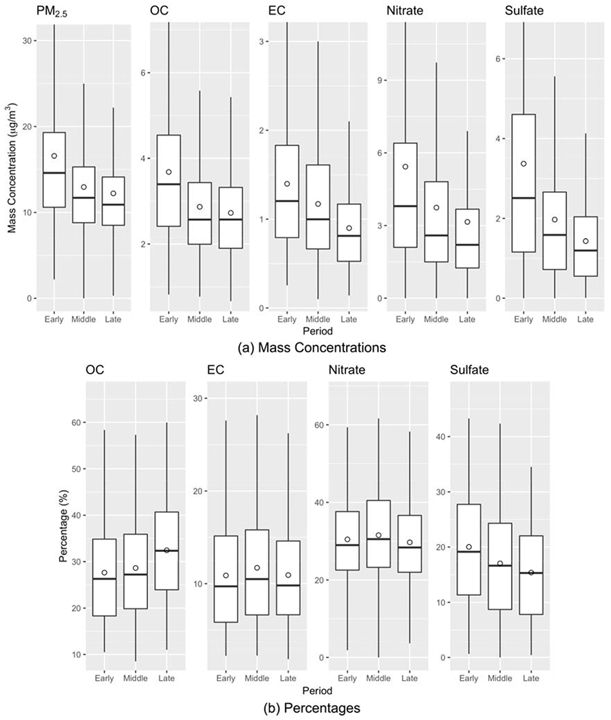
Box plots of (a) mass concentrations of PM2.5 and four major components and (b) percentages of four major components in PM2.5 total mass during the three time periods (EARLY: 2005-2008; MIDDLE: 2009-2012; LATE: 2013-2016). The measurements are the averages of two sub-domains. The box shows the 25th, 50th, and 75th percentiles and the circle shows the mean value.
Figure 1(b) shows the percentage changes of four major PM2.5 components over the time periods. The percentage changes of PM2.5 components in PM2.5 total mass over time were analyzed with the reconstructed PM2.5 mass, i.e., the sum of the masses of 12 components. The percentages of EC and nitrate in PM2.5 total mass were similar over time with means of ~11% and ~30%, respectively. The percentage of sulfate in PM2.5 decreased from 20% in the EARLY period to 15% in the LATE period. A decreased percentage of sulfate over time may reflect the effectiveness of emissions control programs on on-road mobile sources, stationary sources, and changes at the Ports of Long Beach and Los Angeles in fuels and in-port electrification, in which the emission of a major precursor of sulfate, SOx, had a significant reduction (Lurmann et al. 2015). In contrast, the percentage of OC in PM2.5 increased from 28% in the EARLY period to 33% in the LATE period. The increased percentage of OC over time echoes a previous finding that there was a slight increase in secondary organic aerosols (SOAs) as NOx emissions decreased in Los Angeles because non-methane organic gas (NMOG) that previously reacted with NOx was now available to form more SOAs (Zhao et al. 2017). Figure S3 shows the percentage changes of 8 trace components over the time periods. The components contributing to an increasing fraction of PM2.5 mass over time included Br, Ca, Cu, Fe, K, and Si as the total PM2.5 mass concentration declined. The percentage of Zn in PM2.5 remained about the same over time.
3.2. Emergency department visits data
Table 1 summarizes the characteristics of ED patients and numbers of ED visits by health outcome (CVD and asthma), sub-domain (Los Angeles and Rubidoux), and period (EARLY, MIDDLE, and LATE). ED visit totals for CVD and asthma increased by 15% and 12%, respectively, from the EARLY to LATE period in the study domains. Three time periods had similar age structures for two health outcomes. Patients with CVD had a mean age of 65 years (25th, 75th percentiles = [54 years, 79 years]) and those with asthma had a mean age of 28 years (25th, 75th percentiles = [7 years, 46 years]). There was a relatively even split between genders in the CVD and asthma patient populations, with a slight increase in percentage of male patients over time. Patients with CVD and asthma were predominantly white. The structure of race/ethnicity was stable over time. Overall, the characteristics of the ED patients remained relatively consistent over the study period and the increased ED visit numbers might be related to the increased population in Los Angeles (the United States Census Bureau, https://data.census.gov/).
Table 1.
Summary statistics for two health outcomes (CVD and asthma), PM2.5 composition (total mass, four major components, and eight trace components), and weather parameters (daily maximum air temperature and mean dew-point temperature) in Los Angeles and Rubidoux during the three time periods.
| Los Angeles | Rubidoux | |||||
|---|---|---|---|---|---|---|
| EARLY (2005-2008) | MIDDLE (2009-2012) | LATE (2013-2016) | EARLY (2005-2008) | MIDDLE (2009-2012) | LATE (2013-2016) | |
| CVD Cases | ||||||
| N | 277,710 | 292,657 | 308,303 | 77,723 | 104,375 | 111,748 |
| Age (years) | 66.2 (55.0, 80.0)* | 66.4 (55.0, 80.0) | 66.1 (55.0, 79.0) | 61.9 (50.0, 76.0) | 61.9 (51.0, 75.0) | 62.7 (52.0, 75.0) |
| Gender (% male) | 49.1 | 49.4 | 51.3 | 49.0 | 50.8 | 52.0 |
| Race (% white) | 51.0 | 47.8 | 49.2 | 65.7 | 61.4 | 57.3 |
| Asthma Cases | ||||||
| N | 124,577 | 130,657 | 133,717 | 36,085 | 48,899 | 48,444 |
| Age (years) | 28.8 (7.0, 47.0)* | 29.0 (7.0, 48.0) | 29.2 (8.0, 47.0) | 25.8 (7.0, 42.0) | 26.1 (7.0, 43.0) | 27.1 (8.0, 44.0) |
| Gender (% male) | 47.1 | 47.8 | 49.4 | 48.3 | 48.8 | 49.5 |
| Race (% white) | 38.1 | 36.8 | 39.8 | 54.8 | 53.5 | 49.0 |
| Pollutants (μg/m3) | ||||||
| Total PM2.5 | 16.58 (9.55)** | 12.96 (6.73) | 12.21 (6.47) | 18.76 (11.90) | 13.88 (8.70) | 12.48 (7.80) |
| EC | 1.40 (0.79) | 1.17 (0.68) | 0.90 (0.48) | 1.22 (0.80) | 1.01 (0.70) | 0.80 (0.52) |
| OC | 3.68 (1.69) | 2.87 (1.34) | 2.73 (1.18) | 3.51 (1.84) | 2.62 (1.34) | 2.56 (1.22) |
| Nitrate | 5.43 (5.73) | 3.74 (3.40) | 3.15 (3.31) | 7.02 (6.34) | 5.09 (4.58) | 3.74 (3.85) |
| Sulfate | 3.37 (2.91) | 1.97 (1.57) | 1.43 (1.09) | 2.52 (1.94) | 1.63 (1.23) | 1.26 (1.08) |
| Fe | 0.21 (0.17) | 0.20 (0.14) | 0.18 (0.11) | 0.17 (0.13) | 0.14 (0.10) | 0.15 (0.09) |
| S | 1.08 (1.01) | 0.67 (0.52) | 0.52 (0.38) | 0.83 (0.64) | 0.55 (0.41) | 0.44 (0.33) |
| Ca | 0.08 (0.05) | 0.07 (0.05) | 0.06 (0.04) | 0.14 (0.15) | 0.08 (0.05) | 0.08 (0.06) |
| K | 0.12 (0.61) | 0.08 (0.28) | 0.09 (0.32) | 0.12 (0.33) | 0.09 (0.22) | 0.11 (0.45) |
| Si | 0.12 (0.14) | 0.12 (0.11) | 0.11 (0.08) | 0.18 (0.19) | 0.14 (0.11) | 0.16 (0.15) |
| Zn | 0.02 (0.02) | 0.01 (0.01) | 0.01 (0.01) | 0.02 (0.02) | 0.01 (0.01) | 0.01 (0.01) |
| Br | 0.01 (0.00) | 0.00 (0.00) | 0.01 (0.00) | 0.00 (0.00) | 0.01 (0.00) | 0.01 (0.00) |
| Cu | 0.02 (0.02) | 0.01 (0.01) | 0.01 (0.01) | 0.01 (0.02) | 0.01 (0.01) | 0.01 (0.01) |
| Weather Parameters (°C) | ||||||
| Maximum Temperature | 25.0 (19.7, 30.2)* | 24.9 (19.9, 29.4) | 26.4 (21.8, 30.9) | 25.5 (19.6, 31.6) | 25.2 (19.7, 30.8) | 26.2 (21.3, 31.4) |
| Dew-Point Temperature | 8.7 (5.2, 13.3) | 8.7 (5.1, 13.3) | 9.2 (5.2, 14.1) | 6.0 (2.2, 11.1) | 5.9 (2.4, 11.0) | 6.3 (2.0, 11.6) |
Mean (25th, 75th Percentiles)
Mean (Standard Deviation)
3.3. Relative risks associated with PM2.5 total mass
Table 2 and Figure 2(a) show the rate ratios (RRs) and 95% confidence intervals (CIs) for the associations of CVD ED visits and PM2.5 total mass during the three time periods. Both lags 0-3 and 0-7 showed a similar increasing trend over time, where the risk estimates of CVD ED visits associated PM2.5 were smaller in the EARLY period and larger in the later periods. For lag 0-3, the RR in the LATE period (1.020, 95% CI = [1.010, 1.030]) was significantly larger than that in the EARLY period (1.003, [0.996, 1.010]) (Table 2). For lag 0-7, all three period-specific RRs were significantly different. Figure 2(b)–(c) show the age-specific risk estimates of CVD ED visits associated with PM2.5 during the three time periods. The age groups only included ages of 19-64 and 65+ because there were very few ED visits for CVD under the age of 18 (< 2 visits per day on average). The two age groups showed a similar trend in RR across time periods as the all-age analysis where the RRs increased significantly over time. Figure 2(d)–(e) show the season-specific risk estimates of CVD ED visits associated with PM2.5 during the three time periods. Trends in RRs across time periods for each season were similar to those observed for the year-round analysis.
Table 2.
Rate ratios (95% confidence intervals) of PM2.5 and CVD and asthma ED visits (per 10 μg/m3 increase in PM2.5 concentration).
| Outcome | Lag | Period | Rate Ratio (95% Confidence Interval) | Difference of Rate Ratios (95% Confidence Interval) Between Two Periods | |
|---|---|---|---|---|---|
| CVD | 0-3 | EARLY | 1.003 (0.996, 1.010) | MIDDLE – EARLY | 0.0058 (−0.0054, 0.0170) |
| MIDDLE | 1.009 (1.000, 1.018)* | LATE – MIDDLE | 0.0112 (−0.0021, 0.0246) | ||
| LATE | 1.020 (1.010, 1.030)* | LATE – EARLY | 0.0170 (0.0049, 0.0292)* | ||
| 0-7 | EARLY | 0.991 (0.981, 1.002) | MIDDLE – EARLY | 0.0190 (0.0027, 0.0354)* | |
| MIDDLE | 1.010 (0.998, 1.023) | LATE – MIDDLE | 0.0223 (0.0023, 0.0423)* | ||
| LATE | 1.033 (1.017, 1.049)* | LATE – EARLY | 0.0413 (0.0227, 0.0599)* | ||
| Asthma | 0-3 | EARLY | 1.018 (1.006, 1.029)* | MIDDLE – EARLY | −0.0311 (−0.0497, −0.0125)* |
| MIDDLE | 0.986 (0.972, 1.001) | LATE – MIDDLE | 0.0171 (−0.0046, 0.0388) | ||
| LATE | 1.003 (0.988, 1.020) | LATE – EARLY | −0.0140 (−0.0336, 0.0056) | ||
| 0-7 | EARLY | 1.036 (1.018, 1.056)* | MIDDLE – EARLY | −0.0553 (−0.0846, −0.0260)* | |
| MIDDLE | 0.981 (0.959, 1.003) | LATE – MIDDLE | 0.0173 (−0.0179, 0.0525) | ||
| LATE | 0.998 (0.971, 1.025) | LATE – EARLY | −0.0380 (−0.0704, −0.0056)* | ||
Statistically significant at an alpha level of 0.05
Figure 2:
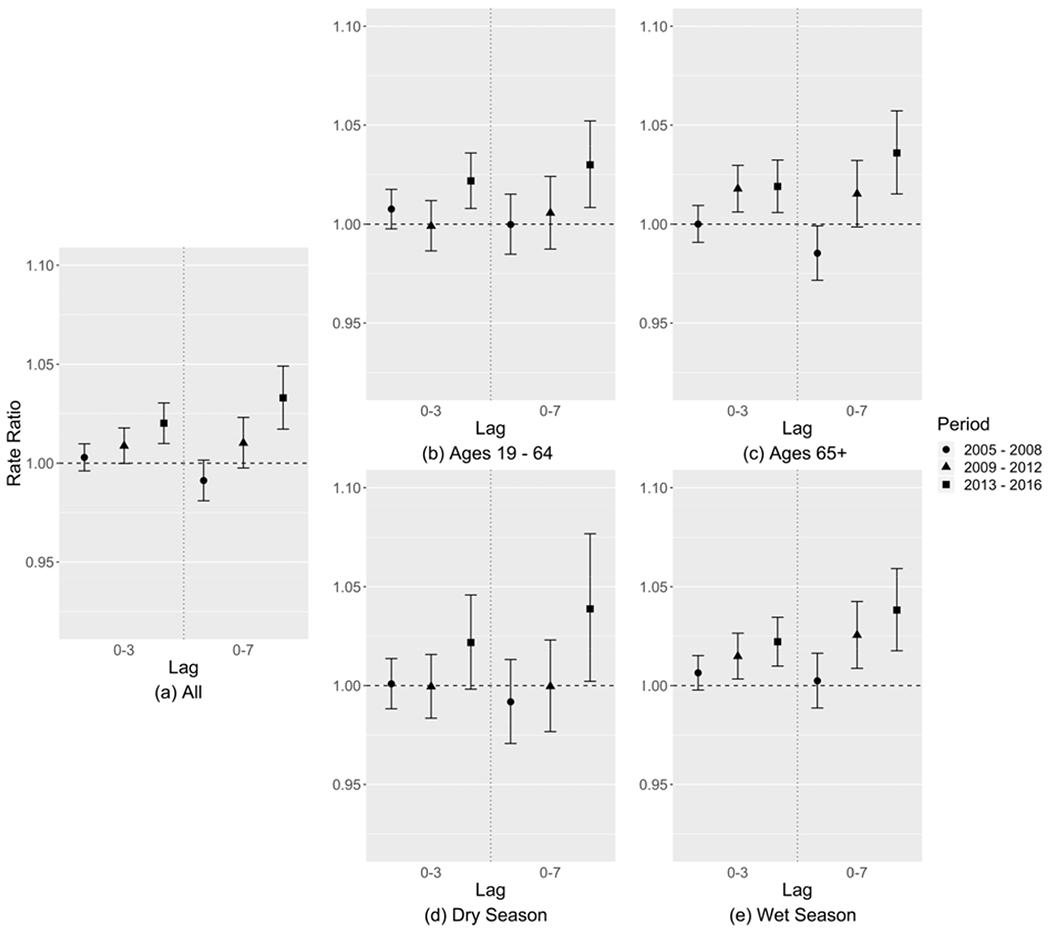
Relative risk estimates of CVD ED visits associated with each 10 μg/m3 increase in PM2.5 mass concentration of (a) all patients, (b) patients of ages 19-64, (c) patients of ages 65+, (d) dry season, and (e) wet season, shown as rate ratios (dots) and 95% confidence intervals (whiskers).
Table 2 and Figure 3(a) show the RRs with 95% CIs for the associations of asthma ED visits and PM2.5 total mass during the three time periods. Both lag structures showed a similar pattern over time, where in contrast to the results for CVD the EARLY period had the largest and significant RRs (lag 0-3: 1.018, [1.006, 1.029]; lag 0-7: 1.036, [1.018, 1.056]) compared to the following two time periods. Figure 3(b)–(c) show the age-specific risk estimates during the three time periods for ages of 1-18 and 19-64, respectively. The RRs in the elderly group (ages 65+) had large 95% CIs because of a small sample size (~10 visits per day on average) and are not shown in the figure. Adult groups (ages 1-18 and 19-64) had a similar trend in RR to the all-age analysis where the RRs were largest in the EARLY period. For children (ages 1-18), the risk estimates of asthma ED visits associated with PM2.5 were similar in the EARLY and LATE periods, and smaller in the MIDDLE period, while the 95% CIs were large. Figure 3(d)–(e) show the season-specific risk estimates during the three time periods. Trends in RRs across time periods for each season were similar to those observed for the year-round analysis.
Figure 3:
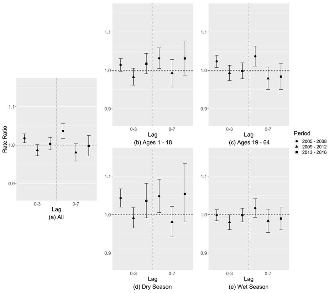
Relative risk estimates of asthma ED visits associated with each 10 μg/m3 increase in PM2.5 mass concentration of (a) all patients, (b) patients of ages 1-18, (c) patients of ages 19-64, (d) dry season, and (e) wet season, shown as rate ratios (dots) and 95% confidence intervals (whiskers).
3.4. Relative risks associated with PM2.5 components
For each PM2.5 component, we ran a two-pollutant model that included the PM2.5 component of interest and the remaining PM2.5 mass (PM2.5 – that specific PM2.5 component). Due to sparser observations and the use of moving averages, PM2.5 component concentrations had less temporal variation, resulting in larger uncertainties than that of PM2.5 total mass.
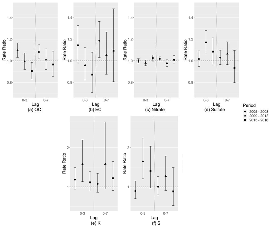
Figure 4 shows the relative risk estimates of CVD ED visits associated with each 10 μg/m3 increase in PM2.5 component concentration, controlling for the remaining PM2.5 mass. OC and nitrate showed a similar increasing trend in RR over time to PM2.5 total mass (Figure 2(a)). EC, Fe, and Ca showed small RRs which tended to be less than 1.0 in the EARLY period and close to 1.0 in the following periods. Sulfate and S had a high correlation (r = 0.95) during the study period so they had a similar pattern, where the RRs were largest and significant in the EARLY period and close to 1.0 in the later periods. The relative risk associated with Si was less than 1.0 and not significant. K had a unique pattern where the MIDDLE period tended to have the largest risk though with a large uncertainty. Figure 5 shows the relative risk estimates of asthma ED visits associated with each 10 μg/m3 increase in PM2.5 component concentration, controlling for the remaining PM2.5 mass. Nitrate, OC, and EC showed a similar pattern to PM2.5 total mass where the EARLY period had the largest RRs. For sulfate, S, and K, the MIDDLE-period RRs tended to be largest and significant. Associations of Zn, Br, and Cu with CVD and associations of Fe, Ca, Si, Zn, Br, and Cu with asthma were consistent with the null (RR = 1.0), with large uncertainties in risk estimates, which are not shown in the results.
Figure 4:
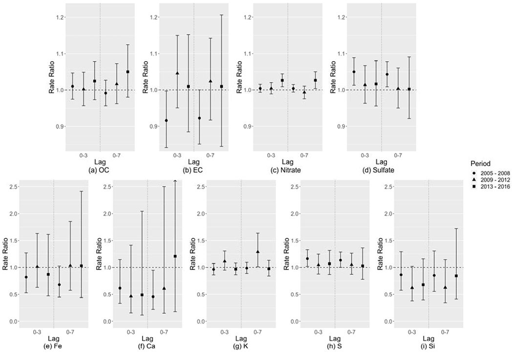
Relative risk estimates of CVD ED visits associated with each 10 μg/m3 increase in PM2.5 component concentration, controlling for the remaining PM2.5 mass, shown as rate ratios (dots) and 95% confidence intervals (whiskers).
Figure 5:
Relative risk estimates of asthma ED visits associated with each 10 μg/m3 increase in PM2.5 component concentration, controlling for the remaining PM2.5 mass, shown as rate ratios (dots) and 95% confidence intervals (whiskers).
Overall, this analysis demonstrated temporal variation in the risk of CVD and asthma ED visits associated with short-term increases in PM2.5 component concentrations. Given that these PM2.5 components are less complex in terms of composition than the PM2.5 mixture and that their toxicities should be less variant over time, the observed temporal variation in relative risk suggests that these components might still be proxies of some complex mixtures.
3.5. Relative risks associated with the remaining PM2.5 mass
Figure S4 shows the relative risk estimates of CVD ED visits associated with each 10 μg/m3 increase in the remaining PM2.5 mass concentration (i.e., β2 in Eq. 2). Apart from nitrate, the remaining PM2.5 mass for all other components showed a similar pattern to PM2.5 total mass. For nitrate, all RRs were close to 1.0 and not statistically significant, which might be caused by unstable estimated coefficients due to a high correlation between PM2.5 total mass and nitrate (r = 0.88). Figure S5 shows the relative risk estimates of asthma ED visits associated with increased remaining PM2.5 mass concentrations. Similarly, the remaining PM2.5 mass was similar to PM2.5 total mass in terms of the temporal trend of RRs, and some variation might happen by chance (e.g., OC) or due to a high correlation with PM2.5 total mass (e.g., nitrate). In general, for all formulations of remaining PM2.5 mass, the temporal trends in relative risk were similar to that of PM2.5 total mass, thus indicating that no single PM2.5 component (when removed from the PM2.5 mixture) was an obvious contributor to those trends.
3.6. Sensitivity analysis
With different degrees of freedom (df = 2-6) of cubic splines of daily maximum air temperature and mean dew-point temperature, the relative risk estimates of CVD and asthma ED visits associated with PM2.5 were consistent (Figure S6). When adding daily minimum air temperature (df = 4) as another confounder, most of the risk estimates were stable apart from the risk of CVD ED visits in the MIDDLE period (Figure S7). However, the RRs were still within the original 95% CIs, indicating that the change might happen by chance. Figures S8 and S9 show that the risk estimates were consistent with different annual knots in time splines and in redefined time periods, respectively. After controlling for ozone, the risk estimates remained consistent (Figure S10). Finally, there were no significant associations between tomorrow’s pollutant levels (lag −1) and today’s ED visits when controlling for today’s pollutant levels (lag 0), and the lag 0 RRs and 95% CIs remained about the same before and after adding tomorrow’s pollutant levels.
4. Discussion
In this study, we analyzed temporal changes in the risk of CVD and asthma ED visits associated with short-term increases in PM2.5 concentrations in Los Angeles, California. This study focused on the period of 2005-2016 during which comprehensive emissions control programs and economic drivers influenced air quality in the region. Similar to previous studies on short-term associations between PM2.5 and CVD (Kirrane et al. 2019) and asthma (Fan et al. 2016; Zheng et al. 2015) health events, a significantly increased risk of CVD and asthma ED visits associated with increases in PM2.5 concentrations were observed. More importantly, we also observed temporal variation in the relative risk with changes in PM2.5 concentrations and composition.
For CVD ED visits, the relative risk estimates were significantly larger in the LATE (2013-2016) compared to the EARLY (2005-2008) period. The estimated 4-day exposure (lag 0-3) RR increased from 1.003 to 1.020 and 8-day exposure (lag 0-7) RR increased from 0.991 to 1.033 per 10 μg/m3 increase in PM2.5 concentration between the EARLY and LATE periods. For asthma ED visits, the largest RRs were found in the EARLY period (lag 0-3 RR = 1.018; lag 0-7 RR = 1.036) while the RRs were smaller in the following periods. In general, there were significant temporal trends in the risk of CVD and asthma ED visits associated with each 10 μg/m3 increase in PM2.5 concentration, and the trends were similar for different lag times (lags 03 and 0-7), age groups (ages 1-18, 19-64, and 65+), and seasons (dry and wet).
The temporal variation in PM2.5 relative risks could be a result of a number of factors, among which changes in PM2.5 composition could be an important one. With two-pollutant models, we investigated the hypothesis that changes in PM2.5 relative risks were associated with changing fractions of individual PM2.5 components in PM2.5 total mass over time. We hypothesized that if the relative risk of CVD and asthma ED visits associated with a PM2.5 mixture without a certain PM2.5 component remained about the same across time periods, then this would be support to show that the component in question was a contributor to the observed temporal variation in relative risk. However, we found that the remaining PM2.5 mass without individual components still had temporal variation in relative risk as PM2.5 total mass, indicating that the observed temporal variation might not be caused by any single component. Another possibility is that the observed temporal variation could result from changing fractions of a group of PM2.5 components acting on different physiological mechanisms. To examine this hypothesis, a multipollutant model should be used to analyze the overall association between multiple PM2.5 components and a health outcome. However, due to the high correlations between different PM2.5 components, multicollinearity could inflate the uncertainty of risk estimates (Gibson et al. 2019). Subtracting multiple components from the total PM2.5 could be another way to assess the hypothesis, but as these components had distinct measurement uncertainties, the cumulative error in the generated remaining PM2.5 mass concentrations could make the risk estimates unreliable. Given these limitations, novel and robust statistical approaches for mixtures are needed to further analyze the combinations of PM2.5 components affecting PM2.5 relative risks (Taylor et al. 2016).
Despite the fact that no single component was identified as an obvious contributor to the temporal variation in the risk of CVD and asthma ED visits associated with short-term increases in PM2.5 concentrations, the component-specific risk estimates still exhibited unique temporal patterns, some of which were different from the pattern of PM2.5 total mass. For example, the risk of CVD ED visits associated with increased OC concentrations had an increasing trend over time, which coincided with the increasing percentage of OC in PM2.5 total mass (OC was the only major component with an increasing percentage of PM2.5 total mass over time). An increasing percentage of OC might include both reactive oxygen species and species with oxidative potential, which could potentially result in increased oxidative stress and exacerbation of cardiorespiratory diseases (Hopke et al. 2015). Previous studies conducted in New York State also suggested that secondary OC could be a key component leading to temporal changes in the risk of adverse health outcomes associated with PM2.5 as oxidative stress is associated more with secondary organic aerosols (Croft et al. 2019; Hopke et al. 2019; Zhang et al. 2018). However, even though increased oxidative stress could be a plausible explanation for the larger risk of CVD ED visits associated with PM2.5 over time, it is difficult to explain the smaller risk of asthma ED visits over time. The inconsistent patterns in different health outcomes indicate that (1) it is possible that secondary OC may have different effects on CVD and asthma, (2) there could be other unmeasured factors leading to different risks of different health outcomes associated with OC, or (3) confounding from co-exposure to other pollutants that impact CVD and asthma not fully captured by the model. Besides, due to the lack of source-specific measurements or predictions for secondary OC levels in Los Angeles, we were not able to fully examine its role in the observed temporal variation in relative risk in this study. Additional source apportionment research will be needed to further analyze secondary OC and its health effects.
In southern California, sulfate could be a proxy of pollution mixtures related to the combustion of sulfur-containing fuel from motor vehicles, locomotives, ships, and off-road diesel equipment. Residual oil would be a prevalent sulfate source in this region especially at the early end of the study period when the ships started to be forced to switch to lower sulfur-containing fuel. Rich et al. (2019) found that residual oil particles and exhaust gas from spark-ignition and diesel vehicles were associated with increased rates of CVD hospitalizations over the next day. In this analysis, the risk of CVD ED visits associated with increased sulfate concentrations was large and significant in the EARLY period and decreased over time. Since these fuel combustion sources had been well-controlled due to the emissions control programs during the study period (Lurmann et al. 2015), it is expected that their adverse effects on CVD could be mitigated.
However, sulfate was associated with asthma ED visits in a different manner, where the MIDDLE period (2009-2012) seemed to have the largest risk. Again, this inconsistency may be caused by different effects of sulfate on different health outcomes, other unmeasured time-variant factors, or confounding from co-exposure to uncaptured pollutants.
The temporal trends in the risk estimates of both CVD and asthma ED visits associated with increased K concentrations were similar, where the largest risk was in the MIDDLE period. K has been extensively used as an indicator of biomass burning (Li et al. 2003), and the MIDDLE period had the lowest mean K concentration associated with fewer wildfire events in southern California. This pattern indicates that the risk associated with emission sources containing K was largest when there were fewer wildfire events and lower K concentrations, which was not expected. Therefore, further research is needed to confirm this health association.
Based on the observed evidence, we infer that other measured or unmeasured time-variant factors, in addition to changes in PM2.5 composition, may also play an important role in the change in PM2.5 relative risks over time. Asthma may be exacerbated by respiratory infections such as influenza, which can cause inflammation of the airways (Glezen 2006). Although we controlled for the ED visit counts for influenza in the asthma models, it was still possible that the control was insufficient due to potential under-detection and under-diagnosis of influenza (Hartman et al. 2018; Thompson et al. 2019). Exposure misclassification could be another potential factor. If the PM2.5 measurements at the monitoring stations were a more representative of population exposures within the respective monitor-buffers in some periods than others, there would be a smaller estimation bias in these periods. However, we would expect such differential exposure misclassification to affect the risk of both CVD and asthma ED visits and thus should not be a major factor influencing the observed differences in temporal patterns of two health outcomes. Other time-variant factors such as changes in population vulnerability (e.g., socioeconomic conditions and underlying diseases) and health care accessibility could also be potential effect modifiers for short-term PM2.5-cardiorespiratory associations. A full investigation of these factors needs detailed community-level information, which warrants further research.
While previous studies reported that PM2.5-cardiorespiratory disease associations may vary by region and sub-populations (Baxter et al. 2013; Davis et al. 2011), this study provides further evidence that these associations may also vary by time, and changes in PM2.5 composition related to emissions control programs and economic changes could be an important driving factor. Apart from those already mentioned, there were several additional limitations in this study. First, the remaining PM2.5 mass concentrations generated by subtracting the mass of individual components from PM2.5 total mass might have some uncertainty due to different measurement errors in different PM2.5 components. This uncertainty might bias the estimated health associations of both the component and the remaining PM2.5 parts. In addition, our exposure assignment relying on central air quality stations might result in exposure misclassification, which was a combination of Berkson and classical error. The moving average method dealing with temporal sparsity in the component measurements was another possible source of exposure misclassification. While the simulations of PM2.5 composition generated by chemical transport models (CTMs) have complete spatiotemporal coverage, their large uncertainty (especially for trace components) resulted from inaccurate emission inventories and source profiles limits their use in epidemiological studies (Hu et al. 2014). Exposure misclassification could result in a bias toward the null and underestimated health associations (Zeger et al. 2000). The temporal sparsity in PM2.5 component data, especially for trace components, may be alleviated in the future with more advanced measurement techniques and more accurate CTMs. Finally, the diagnosis classification codes changed on October 1, 2015, from ICD-9 to ICD-10, might be an additional potential concern. However, all ICD-9 and ICD-10 codes were carefully reviewed to ensure consistency of disease groups, and any outcome misclassification should be minimal.
5. Conclusions
In this study, we observed temporal changes in the risk of CVD and asthma ED visits associated with short-term increases in PM2.5 mass and component concentrations. These temporal changes could be related to changes in the PM2.5 mixtures such as the increasing fraction of OC and the decreasing fraction of sulfate in PM2.5 total mass resulted from comprehensive emissions control programs and economic changes. However, the evidence at the single-component level was not clear. Other factors such as improvements in healthcare and differential exposure misclassification might also contribute to the temporal changes. The complex relationship between changes in the PM2.5 mixture and different health outcomes warrants further validations in other geographical regions.
Supplementary Material
Highlights.
Temporal variations in PM2.5 health associations with CVD and asthma were observed
Changes in PM2.5 health associations may be related to changes in PM2.5 composition
Other factors such as improvements in healthcare may also contribute to the changes
Acknowledgments
This research was supported by the National Institute of Environmental Health Sciences of the National Institutes of Health under award number R01-ES027892. The content is solely the responsibility of the authors and does not necessarily represent the official views of the National Institutes of Health. We acknowledge Shannon Moss at Emory University for assisting us in the health data acquisition and maintenance.
Footnotes
Publisher's Disclaimer: This is a PDF file of an unedited manuscript that has been accepted for publication. As a service to our customers we are providing this early version of the manuscript. The manuscript will undergo copyediting, typesetting, and review of the resulting proof before it is published in its final form. Please note that during the production process errors may be discovered which could affect the content, and all legal disclaimers that apply to the journal pertain.
References
- Abrams JY, Klein M, Henneman LRF, Sarnat SE, Chang HH, Strickland MJ, Mulholland JA, Russell AG, & Tolbert PE (2019). Impact of air pollution control policies on cardiorespiratory emergency department visits, Atlanta, GA, 1999-2013. Environment international, 126(627–634, 10.1016/j.envint.2019.01.052 [DOI] [PubMed] [Google Scholar]
- Baxter LK, Duvall RM, & Sacks J (2013). Examining the effects of air pollution composition on within region differences in PM2.5 mortality risk estimates. Journal of Exposure Science & Environmental Epidemiology, 23(5), 457–465, 10.1038/jes.2012.114 [DOI] [PubMed] [Google Scholar]
- Bell ML, Dominici F, Ebisu K, Zeger SL, & Samet JM (2007). Spatial and temporal variation in PM2.5 chemical composition in the United States for health effects studies. Environmental health perspectives, 115(7), 989–995, 10.1289/ehp.9621 [DOI] [PMC free article] [PubMed] [Google Scholar]
- Bell ML, Ebisu K, Peng RD, Samet JM, & Dominici F (2009). Hospital Admissions and Chemical Composition of Fine Particle Air Pollution. American journal of respiratory and critical care medicine, 179(12), 1115–1120, 10.1164/rccm.200808-1240OC [DOI] [PMC free article] [PubMed] [Google Scholar]
- Bell ML, Samet JM, & Dominici F (2004). Time-series studies of particulate matter. Annual Review of Public Health, 25(247–280, 10.1146/annurev.publhealth.25.102802.124329 [DOI] [PubMed] [Google Scholar]
- Bell ML, Zanobetti A, & Dominici F (2013). Evidence on Vulnerability and Susceptibility to Health Risks Associated With Short-Term Exposure to Particulate Matter: A Systematic Review and Meta-Analysis. American journal of epidemiology, 178(6), 865–876, 10.1093/aje/kwt090 [DOI] [PMC free article] [PubMed] [Google Scholar]
- Brook RD, Franklin B, Cascio W, Hong YL, Howard G, Lipsett M, Luepker R, Mittleman M, Samet J, Smith SC, & Tager I (2004). Air pollution and cardiovascular disease - A statement for healthcare professionals from the expert panel on population and prevention science of the American Heart Association. Circulation, 109(21), 2655–2671, 10.1161/01.Cir.0000128587.30041.C8 [DOI] [PubMed] [Google Scholar]
- Casillas AM, Hiura T, Li N, & Nel AE (1999). Enhancement of allergic inflammation by diesel exhaust particles: permissive role of reactive oxygen species. Annals of Allergy Asthma & Immunology, 83(6), 624–629, 10.1016/s1081-1206(10)62884-0 [DOI] [PubMed] [Google Scholar]
- Cho CC, Hsieh WY, Tsai CH, Chen CY, Chang HF, & Lin CS (2018). In Vitro and In Vivo Experimental Studies of PM2.5 on Disease Progression. International Journal of Environmental Research and Public Health, 15(7), 1380, 10.3390/ijerph15071380 [DOI] [PMC free article] [PubMed] [Google Scholar]
- Croft DP, Zhang WJ, Lin S, Thurston SW, Hopke PK, Masiol M, Squizzato S, van Wijngaarden E, Utell MJ, & Rich DQ (2019). The Association between Respiratory Infection and Air Pollution in the Setting of Air Quality Policy and Economic Change. Annals of the American Thoracic Society, 16(3), 321–330, 10.1513/AnnalsATS.201810-691OC [DOI] [PMC free article] [PubMed] [Google Scholar]
- Davis JA, Meng Q, Sacks JD, Dutton SJ, Wilson WE, & Pinto JP (2011). Regional variations in particulate matter composition and the ability of monitoring data to represent population exposures, 409(23), 5129–5135, 10.1016/j.scitotenv.2011.08.013 [DOI] [PubMed] [Google Scholar]
- Devlin RB, Duncan KE, Jardim M, Schmitt MT, Rappold AG, & Diaz-Sanchez D (2012). Controlled Exposure of Healthy Young Volunteers to Ozone Causes Cardiovascular Effects. Circulation, 126(1), 104–111, 10.1161/circulationaha.112.094359 [DOI] [PubMed] [Google Scholar]
- Dolislager LJ, & Motallebi N (1999). Characterization of particulate matter in California. Journal of the Air & Waste Management Association, 49(45–56, 10.1080/10473289.1999.10463898 [DOI] [PubMed] [Google Scholar]
- Dominici F, Peng RD, Ebisu K, Zeger SL, Samet JM, & Bell ML (2007). Does the effect of PM10 on mortality depend on PM nickel and vanadium content? A reanalysis of the NMMAPS data. Environmental health perspectives, 115(12), 1701–1703, <Go to ISI>://WOS:000251411500027 [DOI] [PMC free article] [PubMed] [Google Scholar]
- Fan J, Li S, Fan C, Bai Z, & Yang K (2016). The impact of PM2.5 on asthma emergency department visits: a systematic review and meta-analysis. Environmental Science and Pollution Research, 23(1), 843–850, 10.1007/s11356-015-5321-x [DOI] [PubMed] [Google Scholar]
- Flanders WD, Klein M, Darrow LA, Strickland MJ, Sarnat SE, Sarnat JA, Waller LA, Winquist A, & Tolbert PE (2011). A method for detection of residual confounding in time-series and other observational studies. Epidemiology, 22(1), 59–67, 10.1097/EDE.0b013e3181fdcabe [DOI] [PMC free article] [PubMed] [Google Scholar]
- Gibson EA, Nunez Y, Abuawad A, Zota AR, Renzetti S, Devick KL, Genning C, Goldsmith J, Coull BA, & Kioumourtzoglou MA (2019). An overview of methods to address distinct research questions on environmental mixtures: an application to persistent organic pollutants and leukocyte telomere length. Environmental Health, 18(1) 10.1186/s12940-019-0515-1 [DOI] [PMC free article] [PubMed] [Google Scholar]
- Glezen W (2006). Asthma, influenza, and vaccination. Journal of Allergy and Clinical Immunology, 118(6), 1199–1206, 10.1016/j.jaci.2006.08.032 [DOI] [PubMed] [Google Scholar]
- Guarnieri M, & Balmes JR (2014). Outdoor air pollution and asthma. Lancet, 383(9928), 1581–1592, 10.1016/s0140-6736(14)60617-6 [DOI] [PMC free article] [PubMed] [Google Scholar]
- Halonen JI, Lanki T, Yli-Tuomi T, Kulmala M, Tiittanen P, & Pekkanen J (2008). Urban air pollution, and asthma and COPD hospital emergency room visits. Thorax, 63(7), 635–641, 10.1136/thx.2007.091371 [DOI] [PubMed] [Google Scholar]
- Hartman L, Zhu Y, Edwards KM, Griffin MR, & Talbot HK (2018). Underdiagnosis of Influenza Virus Infection in Hospitalized Older Adults. Journal of the American Geriatrics Society 10.1111/jgs.15298 [DOI] [PMC free article] [PubMed] [Google Scholar]
- Hopke PK, Croft D, Zhang WJ, Lin S, Masiol M, Squizzato S, Thurston SW, van Wijngaarden E, Utell MJ, & Rich DQ (2019). Changes in the acute response of respiratory diseases to PM2.5 in New York State from 2005 to 2016. Science of the Total Environment, 677(328–339, 10.1016/j.scitotenv.2019.04.357 [DOI] [PubMed] [Google Scholar]
- Hopke PK, Kane C, Utell MJ, Chalupa DC, Kumar P, Ling F, Gardner B, & Rich DQ (2015). Triggering of myocardial infarction by increased ambient fine particle concentration: Effect modification by source direction, 142(374–379, 10.1016/j.envres.2015.06.037 [DOI] [PMC free article] [PubMed] [Google Scholar]
- Hu JL, Zhang HL, Chen SH, Wiedinmyer C, Vandenberghe F, Ying Q, & Kleeman MJ (2014). Predicting Primary PM2.5 and PM0.1 Trace Composition for Epidemiological Studies in California. Environmental science & technology, 48(9), 4971–4979, 10.1021/es404809j [DOI] [PubMed] [Google Scholar]
- Ji M, Cohan DS, & Bell ML (2011). Meta-analysis of the association between short-term exposure to ambient ozone and respiratory hospital admissions. Environmental Research Letters, 6(2) 10.1088/1748-9326/6/2/024006 [DOI] [PMC free article] [PubMed] [Google Scholar]
- Kim H, Kim H, Park YH, & Lee JT (2017). Assessment of temporal variation for the risk of particulate matters on asthma hospitalization. Environmental research, 156(542–550, 10.1016/j.envres.2017.04.012 [DOI] [PubMed] [Google Scholar]
- Kim SY, Peel JL, Hannigan MP, Dutton SJ, Sheppard L, Clark ML, & Vedal S (2012). The Temporal Lag Structure of Short-term Associations of Fine Particulate Matter Chemical Constituents and Cardiovascular and Respiratory Hospitalizations. Environmental health perspectives, 120(8), 1094–1099, 10.1289/ehp.1104721 [DOI] [PMC free article] [PubMed] [Google Scholar]
- Kirrane EF, Luben TJ, Benson A, Owens EO, Sacks JD, Dutton SJ, Madden M, & Nichols JL (2019). A systematic review of cardiovascular responses associated with ambient black carbon and fine particulate matter. Environment international, 127(305–316, 10.1016/j.envint.2019.02.027 [DOI] [PMC free article] [PubMed] [Google Scholar]
- Li J, Pósfai M, Hobbs PV, & Buseck PR (2003). Individual aerosol particles from biomass burning in southern Africa: 2, Compositions and aging of inorganic particles. Journal of Geophysical Research: Atmospheres, 108(D13) 10.1029/2002jd002310 [DOI] [Google Scholar]
- Lippmann M, Ito K, Hwang JS, Maciejczyk P, & Chen LC (2006). Cardiovascular effects of nickel in ambient air. Environmental health perspectives, 114(11), 1662–1669, 10.1289/ehp.9150 [DOI] [PMC free article] [PubMed] [Google Scholar]
- Lu F, Xu DQ, Cheng YB, Dong SX, Guo C, Jiang X, & Zheng XY (2015). Systematic review and meta-analysis of the adverse health effects of ambient PM2.5 and PM10 pollution in the Chinese population. Environmental research, 136(196–204, 10.1016/j.envres.2014.06.029 [DOI] [PubMed] [Google Scholar]
- Lurmann F, Avol E, & Gilliland F (2015). Emissions reduction policies and recent trends in Southern California’s ambient air quality. Journal of the Air & Waste Management Association, 65(3), 324–335, 10.1080/10962247.2014.991856 [DOI] [PMC free article] [PubMed] [Google Scholar]
- Rich DQ, Zhang W, Lin S, Squizzato S, Thurston SW, Van Wijngaarden E, Croft D, Masiol M, & Hopke PK (2019). Triggering of cardiovascular hospital admissions by source specific fine particle concentrations in urban centers of New York State. Environment international, 126(387–394, 10.1016/j.envint.2019.02.018 [DOI] [PMC free article] [PubMed] [Google Scholar]
- Solomon PA, Crumpler D, Flanagan JB, Jayanty RKM, Rickman EE, & McDade CE (2014). U.S. National PM 2.5 Chemical Speciation Monitoring Networks—CSN and IMPROVE: Description of networks, 64(12), 1410–1438, 10.1080/10962247.2014.956904 [DOI] [PubMed] [Google Scholar]
- Squizzato S, Masiol M, Rich DQ, & Hopke PK (2018). PM2.5 and gaseous pollutants in New York State during 2005-2016: Spatial variability, temporal trends, and economic influences. Atmospheric Environment, 183(209–224, 10.1016/j.atmosenv.2018.03.045 [DOI] [Google Scholar]
- Sun QH, Wang AX, Jin XM, Natanzon A, Duquaine D, Brook RD, Aguinaldo JGS, Fayad ZA, Fuster V, Lippmann M, Chen LC, & Rajagopalan S (2005). Long-term air pollution exposure and acceleration of atherosclerosis and vascular inflammation in an animal model. Jama-Journal of the American Medical Association, 294(23), 3003–3010, 10.1001/jama.294.23.3003 [DOI] [PubMed] [Google Scholar]
- Taylor KW, Joubert BR, Braun JM, Dilworth C, Gennings C, Hauser R, Heindel JJ, Rider CV, Webster TF, & Carlin DJ (2016). Statistical Approaches for Assessing Health Effects of Environmental Chemical Mixtures in Epidemiology: Lessons from an Innovative Workshop. Environmental health perspectives, 124(12) 10.1289/ehp547 [DOI] [PMC free article] [PubMed] [Google Scholar]
- Thompson MG, Levine MZ, Bino S, Hunt DR, Al-Sanouri TM, Simoes EAF, Porter RM, Biggs HM, Gresh L, Simaku A, Abu Khader I, Tallo VL, Meece JK, McMorrow M, Mercado ES, Joshi S, DeGroote NP, Hatibi I, Sanchez F, Lucero MG, Faouri S, Jefferson SN, Maliqari N, Balmaseda A, Sanvictores D, Holiday C, Sciuto C, Owens Z, Azziz-Baumgartner E, & Gordon A (2019). Underdetection of laboratory-confirmed influenza-associated hospital admissions among infants: a multicentre, prospective study. Lancet Child & Adolescent Health, 3(11), 781–794, 10.1016/s2352-4642(19)30246-9 [DOI] [PMC free article] [PubMed] [Google Scholar]
- Tian YH, Xiang X, Juan J, Sun KX, Song J, Cao YY, & Hu YH (2017). Fine particulate air pollution and hospital visits for asthma in Beijing, China. Environmental pollution, 230(227–233, 10.1016/j.envpol.2017.06.029 [DOI] [PubMed] [Google Scholar]
- Tong D, Pan L, Chen WW, Lamsal L, Lee P, Tang YH, Kim H, Kondragunta S, & Stajner I (2016). Impact of the 2008 Global Recession on air quality over the United States: Implications for surface ozone levels from changes in NOx emissions. Geophysical Research Letters, 43(17), 9280–9288, 10.1002/2016gl069885 [DOI] [Google Scholar]
- Zanobetti A, Schwartz J, & Gold D (2000). Are there sensitive subgroups for the effects of airborne particles? Environmental health perspectives, 108(9), 841–845, 10.2307/3434991 [DOI] [PMC free article] [PubMed] [Google Scholar]
- Zeger SL, Thomas D, Dominici F, Samet JM, Schwartz J, Dockery D, & Cohen A (2000). Exposure measurement error in time-series studies of air pollution: concepts and consequences. Environ Health Perspect, 108(5), 419–426, 10.1289/ehp.00108419 [DOI] [PMC free article] [PubMed] [Google Scholar]
- Zhang WJ, Lin S, Hopke PK, Thurston SW, van Wijngaarden E, Croft D, Squizzato S, Masiol M, & Rich DQ (2018). Triggering of cardiovascular hospital admissions by fine particle concentrations in New York state: Before, during, and after implementation of multiple environmental policies and a recession. Environmental pollution, 242(1404–1416, 10.1016/j.envpol.2018.08.030 [DOI] [PubMed] [Google Scholar]
- Zhao YL, Saleh R, Saliba G, Presto AA, Gordon TD, Drozd GT, Goldstein AH, Donahue NM, & Robinson AL (2017). Reducing secondary organic aerosol formation from gasoline vehicle exhaust. Proceedings of the National Academy of Sciences of the United States of America, 114(27), 6984–6989, 10.1073/pnas.1620911114 [DOI] [PMC free article] [PubMed] [Google Scholar]
- Zheng X-Y, Ding H, Jiang L-N, Chen S-W, Zheng J-P, Qiu M, Zhou Y-X, Chen Q, & Guan W-J (2015). Association between Air Pollutants and Asthma Emergency Room Visits and Hospital Admissions in Time Series Studies: A Systematic Review and Meta-Analysis. PloS one, 10(9), e0138146, 10.1371/journal.pone.0138146 [DOI] [PMC free article] [PubMed] [Google Scholar]
- Zou YJ, Jin CY, Su Y, Li JR, & Zhu BS (2016). Water soluble and insoluble components of urban PM2.5 and their cytotoxic effects on epithelial cells (A549) in vitro. Environmental pollution, 212(627–635, 10.1016/j.envpol.2016.03.022 [DOI] [PubMed] [Google Scholar]
Associated Data
This section collects any data citations, data availability statements, or supplementary materials included in this article.