Risk maps for cities: Incorporating streets into geostatistical models

Abstract

Vector-borne diseases commonly emerge in urban landscapes, and Gaussian field models can be used to create risk maps of vector presence across a large environment. However, these models do not account for the possibility that streets function as permeable barriers for insect vectors. We describe a methodology to transform spatial point data to incorporate permeable barriers, by distorting the map to widen streets, with one additional parameter. We use Gaussian Field models to estimate this additional parameter, and develop risk maps incorporating streets as permeable barriers. We demonstrate our method on simulated datasets and apply it to data on Triatoma infestans, a vector of Chagas disease in Arequipa, Peru. We found that the transformed landscape that best fit the observed pattern of Triatoma infestans infestation, approximately doubled the true Euclidean distance between neighboring houses on different city blocks. Our findings may better guide control of re-emergent insect populations.

1. Introduction

Vector-borne diseases are increasingly common in urban areas, and efforts to control these diseases are often targeted at the vector itself. However, detecting populations of disease vectors in large urban environments is especially complex (Weaver (2013), Knudsen and Slooff (1992)). Poor and unplanned urban environments can create ideal breeding grounds for many vectors, facilitating increased transmission of vector-borne diseases in population dense areas (Knudsen and Slooff (1992), Bowman et al. (2008), Levy et al. (2006)).

This research is motivated by the need to understand vector distribution patterns in Arequipa, the second largest city in Peru. In particular, we are interested in models that can help guide search strategies for Triatoma infestans, a vector of Chagas disease. Chagas disease, which is caused by the parasite Trypansoma cruzi, causes significant mortality in the Americas (Dias et al. (2002), Bern (2015)). T. infestans, the only vector of T. cruzi transmission in Arequipa, is a species of triatomine that has proven well adapted to urban settings. The species prefers environments such as guinea pig pens, common in Peru, and housing materials with dark cracks and crevices (Levy et al. (2006)). Since the insect rarely flies, there is a highly spatial aspect to the observed vector distribution patterns on very fine scales. Previous studies have shown that the vectors are much more likely to move within city blocks than cross a street (Barbu et al. (2013)).

To control the spread of Chagas disease, the regional ministry of Health of Arequipa began an inspection and spray campaign targeting T. infestans in 2003 (Barbu et al. (2014)). Following the campaign, both the prevalence of the parasite and vector populations decreased substantially in metropolitan Arequipa (Barbu et al. (2014)). However, T. infestans are still occasionally observed, and targeted surveillance is ongoing. The ongoing surveillance is multifaceted; residents may report infestations, and in addition, inspectors proactively search households for vectors. Due to the size of Arequipa, inspectors cannot search every household, but must select which ones to search. To guide our prospective searches, we are motivated to develop risk maps, incorporating the geographic location of observed household infestations.

Creating risk maps using Gaussian fields (GFs) is an area of active research and development (Oluwole et al. (2015), Adigun et al. (2015), Jaya et al. (2016)). Until recently, fitting GF models was computationally difficult, due to large matrix calculations (the big n problem) in covariance estimation. However, recent advances in theory and computation, discussed below, have alleviated this problem. Lindgren et al. described the relationship between GFs and Gaussian Markov Random fields (GMRFs); an R package was developed to implement these analyses using nested integrated laplace approximations, easing the computational burden of these models (Blangiardo et al. (2013), Lindgren et al. (2011), Rue et al. (2009)).

However, geostatistical models using Gaussian fields do not typically incorporate the structure of urban landscapes (Diggle et al. (2003)). Several arboviruses, including Dengue, Chikungunya, West Nile, and Zika, have emerged repeatedly in urban areas (Haley (2012), Sikka et al. (2016)). Parasitic diseases, such as malaria and Chagas disease, once considered rural problems, have become common in cities (LaDeau et al. (2015), Delgado et al. (2013)). Including the spatial structure of city streets may more accurately describe spatial associations characteristic of insect infestations and therefore help in developing effective public health interventions to reduce transmission in population dense areas (Weaver (2013)).

In this paper we develop an approach to predict the probability of urban insect vector infestation using a geostatistical model that incorporates city streets as permeable barriers. Our approach estimates the reduced movement of vectors between blocks, compared to within blocks, and predicts the heterogeneous urban vector distributions using a Gaussian field. Our model is computationally efficient and easily adaptable to other cities and vectors. Here, we present our methodology, demonstrate our approach on simulated data, and apply it to data on Chagas disease vectors in a district of the city of Arequipa, Peru.

2. Methods

2.1. Gaussian field approach

In this subsection we review the Gaussian field approach that can be used to create risk maps, ignoring the issue of streets as barriers. Gaussian fields are often used to model various types of point-level data, also known as geostatistical data. These models are popular for their flexibility and ability to capture complex processes across a wide range of applications such as epidemiology, ecology, and imaging (Rossi et al. (1992), Brooker (2007), Diggle et al. (2003)). Using this modeling approach, we assume the data, the presence of T. infestans, is a continuous stochastic process, with observations over a two-dimension landscape, at locations c.

Denote by y_i the indicator variable for vector presence at house i. We can model the probability of vector presence at house i, π_i, using a logistic model with intercept and Gaussian field. Although we do not use any household-level covariates in our model, they can easily be incorporated into the formula (1) with additional regression parameters. We use the model:

$$\begin{gathered} \mathrm{logit}\left({\pi }_i\right)={\beta }_0+u_i \\ \mathit{u}\sim N(0,\mathrm{\Sigma }) \end{gathered}$$ (1)

where u_i is a realization of the GF, x(c_i), and c_i is the location of house i. We use a Matérn covariance structure, which is commonly used in spatial statistics. Specifically, the covariance between u_i and u_j is

$${\mathrm{\Sigma }}_{ij}={\sigma }_u^2\frac{2^{1-\nu }}{\mathrm{\Gamma }(\nu )}{\left(\kappa \Vert c_i-c_j\Vert \right)}^{\nu }{K}_{\nu }\left(\kappa \Vert c_i-c_j\Vert \right)$$

where ${\sigma }_u^2$ is the marginal variance of the random effect, ∥ · ∥ is the Euclidean distance, K_ν is the modified Bessel function of the second order, and κ and ν are parameters. The parameter ν describes the smoothness of the stochastic process and therefore controls the shape of the covariance function (the function is ⌊ν −1⌋ times differentiable). The κ parameter characterizes how quickly the correlation between two points decreases as the distance between them increases, capturing the scale of the relationship.

The Matérn covariance structure has become widely accepted for GF models because of its link to GMRFs (Besag (1975), Rue and Held (2005), Rue et al. (2009), Lindgren et al. (2011)). Using the Matérn covariance, x(c) is a solution to the linear fractional stochastic partial differential equation (SPDE):

$$W(\mathit{c})=x(\mathit{c}){\left({\kappa }^2-\mathrm{\Delta }\right)}^{\alpha /2}$$

where α = ν + d/2 and Δ is the Laplacian

$$\mathrm{\Delta }=\sum _{i=1}^d\frac{{\partial }^2}{\partial x{(\mathit{c})}_i^2}$$

and d = 2 since $\mathit{c}\in {\Re }^2$ (Whittle (1954), Whittle (1963)).

Using this solution, Lindgren et al. (2011) found a direct link between the GF and GMRF, which greatly eases the computational burden of GF estimation. Using this link, we can estimate the precision matrix that represents the GF accurately, over a wide range of marginal variances, with sparse matrix calculations. For more details on this relationship, see Lindgren et al. (2011).

We follow the parameterization of Lindgren et al. (2011) and Krainski and Lindgren (2013), defining the covariance function in terms of θ = {θ₁, θ₂}, functions of κ, the scale parameter, and ${\sigma }_u^2$, the marginal variance:

$${\theta }_1=-\log \left(4\pi {\kappa }^2{\sigma }_u^2\right)/2$$

$${\theta }_2=\log (\kappa )$$

We also fix α, as defined earlier, to α = 2. This setting is a natural choice for two dimensional problems, as argued in Whittle (1954), but researchers may vary the value of α as needed. Together, θ and α define the Matérn covariance, Σ, of the GMRF.

2.2. Incorporating streets as barriers

The Gaussian field assumes a continuous, non-linear, yet smooth relationship between houses as a function of the Euclidean distance between them. However, urban streets create an uneven landscape on which the stochastic process occurs. Previous studies have shown the vector of Chagas disease, T. infestans, is less likely to move between city blocks compared to within blocks (Barbu et al. (2013)).

One option to capture the heterogeneity of the urban grid would be to add a parameter into the covariance function to indicate whether two points are on the same city block as each other. This approach would allow the relationship of the outcome and distance to depend on whether or not streets separate the points. However, the Matérn covariance is the key element that links the GF to GMRF and changing the function itself may impact the relationship, which is key to efficient parameter estimation. We propose an alternative approach that fits into existing GF estimation software and incorporates an additive effect, so if points are separated by multiple streets, the barrier increases.

Our approach uses a single additional parameter, S, that influences the covariance function directly through the distances between houses by distorting the city map. Using S, we create additional Euclidean distances between houses on different blocks, but maintain the Euclidean distances between houses on the same block, creating permeable barriers. We define S as the ratio of the distorted distance between geographic block medians, calculated as the median c of each block, compared to the true distance (Figure 1). This additional distance between blocks influences the model directly through the spatial covariance structure, ∥c_i − c_j∥ by widening the streets between blocks. With this approach, if S is known, the Gaussian field model can be directly used. In addition, this approach has an additive barrier effect, rather than simply an indicator of whether or not two houses are on the same block. If points are more than one block apart, the width of each street between the points is modified. We assume streets do not facilitate improved vector movement and restrict S ≥ 1, with S = 1 representing the true map.

Figure 1:

A) S = 1, which corresponds to the true map of section in Mariano Melgar, Arequipa, Peru used for simulations. There is no map distortion at this scale. B) Distorted map to a scale of S = 1.5, where the distance between geographic medians of blocks are 1.5 fold the true distance. C) Map distorted to scale S = 2.5, where distance between geographic medians of blocks are 2.5 fold the true distance. Note distance between houses within block is maintained but distance between houses on different blocks is stretched.

In other words, S reduces the correlation between houses that are a distance apart but on different city blocks. In practice, this additional parameter is a flexible, usable tool to characterize a heterogeneous landscape using a continuous latent field. On different types of landscapes, S could be used to define other potential permeable barriers such as rivers, valleys, or mountains.

2.3. Estimation and Interpretation

We now describe our approach to incorporate S into the model, interpret the map distortion, and estimate the parameters. Each house i is located on a known city block j. We first mark the spatial center of each block by finding the median coordinates of each block,

$$\{X_j^M,Y_j^M\}=\left\{\mathrm{median}\left(X_j\right),\mathrm{median}\left(Y_j\right)\right\}.$$

We then define the location of each house in relation to the center of the house’s block,

$$\{{\overline{X}}_i,{\overline{Y}}_i\}=\{X_i-X_j^M,Y_i-Y_j^M\}.$$

We stretch the map by moving the block centers by scale S and recording house coordinates relative to the block center, $\left\{{\overline{X}}_i,{\overline{Y}}_i\right\}$, at the true distance. The distorted map coordinates, $\{{\widehat{X}}_j,{\widehat{Y}}_j\}$, become

$$\left\{{\widehat{X}}_i,{\widehat{Y}}_i\right\}=\left\{X_j^{M}S+{\overline{X}}_i,Y_j^{M}S+{\overline{Y}}_i\right\}.$$

This approach retains the block structure but enables the manipulation of blocks relative to each other. The interpretation of the distorted map is somewhat dependent on the map itself due to the irregular size and shape of each individual city block. S describes the additional distance between the geographic median of each city block relative to the true distance. For example, S = 1.5 corresponds to adding 50% of the true distance between the geographic medians of each block. Due to the irregular grid, this distortion corresponds to varying degrees of street distortion depending on the size of the blocks on either side of the street. The effect of the map distortion of the width of streets in the map in Figure 1 is summarized in Table 1. Larger city blocks result in greater distortion because the houses are located farther from the geographic median of the block. If blocks are all the same shape and size, the increase in street width will be proportional for all streets, however this is rare in practice.

Table 1:

Description of map distortion in Figure 1 scaled so the spatial unit is the average distance between nearest neighbors on the same block. Interpretation of S varies by specific map due to variability in sizes and shapes of city blocks. S describes ratio of distance between geographic median of each city block relative to the true map (which is equivalent to S = 1). Table summarizes how this distortion corresponds to additional distance between houses on different blocks using mean and standard deviation (sd). The distortion varies block by block due to irregular grid.

	S = 1	S = 1.5	S = 2.5
Average distance (and sd) between nearest neighbors on the same block (ie. no barrier)	1.0 (0.3)	1.0 (0.3)	1.0 (0.3)
Average distance (and sd) between nearest neighbors on different blocks (ie. one barrier)	3.6 (1.1)	8.0 (1.5)	16.0 (2.3)
Ratio of average distance between nearest neighbors on different blocks compared to same distance when S = 1	-	2.2 (0.4)	4.4 (0.9)

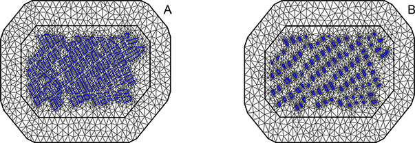
To use the GMRF representation on irregular points, we divide our landscape into non-intersecting triangles, as described in Lindgren et al. (2011). A Delaunay triangulation is created over the landscape, forming a mesh. Each house is located at a vertex in the mesh. To ensure a regular triangulation, the maximum edge length is specified to be 100S to appropriately adjust for map distortion. Although meshes are not identical between grid samples of S, controlling the maximum edge length as a function of S ensures that the triangulation is similar (Figure 2).

Figure 2:

Mesh over the map of the simulation region (houses in blue). Maximum edge length is constrained to 100S to keep meshes consistent between scales. A. S = 1 B. S = 1.5

We implement this methodology using the R package ‘INLA’ (Rue et al. (2009), Rue et al. (2014), Krainski and Lindgren (2013)). The ability of this approach to fit into the existing R package makes the method easy to implement for researchers in different fields. INLA is a relatively new, yet powerful tool, and the package is designed for flexible and complex model development. The package is continually updated to incorporate new developments in spatial statistics. We chose to implement our approach using INLA due to the speed, package flexibility, and ease of implementation for future researchers. The code for our approach is available at https://github.com/chirimacha/Risk-maps-for-cities. We plan to use our method in real-time in the field to guide vector surveillance, and therefore these strengths are of particular significance.

In the last few years, INLA has become a popular method to fit GFs. The algorithm is an alternative to Markov chain Monte Carlo algorithms, which are common for geostatistical models but can be problematic in GF estimation due to non-convergence and long computation times. The latent field u tend to be highly correlated, and u also tend to be dependent on the model hyperparameters, a common issue that arises in MCMC algorithms. Rue et al. found estimation of GMRF models using integrated nested Laplace approximations was more precise and significantly faster (Rue et al. (2009)). This approach uses Gaussian approximations, nested Laplace approximations, and numerical integration to estimate the marginal distributions of the latent field and hyperparameters. The approximations are especially precise for GF estimation. For details on the algorithm, see Rue et al. (2009).

To estimate S, we fit the model at several values of S and compare the log-likelihoods. We estimate S as the value that maximizes the log-likelihood of the model. Using the INLA estimation algorithm, it is not possible to update the estimate of S in the same way as an MCMC algorithm. In addition, changing S changes the mesh used in the model. However, for the purposes of creating risk maps, estimating a full posterior distribution for S does not provide a benefit over using the estimate of S directly.

3. Simulations

To evaluate the performance of our proposed method, we simulate data on a subset of the study region consisting of 2265 houses over 93 city blocks (Figure 1a). Our barrier effect parameter, S, and three parameters (κ, σ_u, β₀) in the model (1) with 2×2×2=8 simulation scenarios with a fixed intercept β₀ = −3 are considered: (1) κ is either 0.005 or 0.01, (2) ${\sigma }_u^2$ is either 5 or 10, and (3) S is either 1.5 or 2.5. Additional simulation scenarios are considered in Appendix A. Each simulated data is generated with respect to the true values of the four parameters in each simulation scenario.

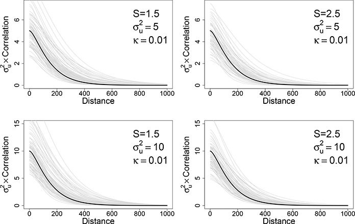
Table 2 shows the simulation results from 100 Monte Carlo simulations for each scenario. The table summarizes the true parameter values, the parameter estimates using our approach, and the proportion of simulations with successful identification of S. It is important to tune the parameters so that they produce realistic infestation patterns; under some parameter regimes, extremely sparse or over-saturated landscapes will be produced. The simulation results demonstrate the ability of this approach to successfully identify S in most cases. In addition, the model captures the covariance function remarkably well, using only observed binary data (Figure 4).

Table 2:

Results from 100 Monte Carlo simulations for each parameter set. The parameter estimates are shown with the corresponding estimated standard deviations with the true values set for the simulations. The coverage of (${\widehat{\beta }}_0$) is the average rate that the credible interval captures the true value of β₀ for identified simulation cases. The last column is the proportion of identifiable simulated datasets.

True values				Estimates
κ	${\mathit{\sigma }}_{\mathit{u}}^{\mathbf{2}}$	S	β0	$\widehat{\mathit{S}}$	${\widehat{\mathit{\beta }}}_{\mathbf{0}}$	Coverage (β0)	Identification (S)
0.005	5	1.5	−3	1.57 (0.35)	−3.11 (0.89)	1.00	0.95
		2.5	−3	2.48 (0.53)	−3.13 (0.61)	1.00	0.73
	10	1.5	−3	1.61 (0.33)	−3.13 (1.26)	0.97	0.98
		2.5	−3	2.77 (0.55)	−3.05 (0.94)	0.97	0.89
0.01	5	1.5	−3	1.64 (0.27)	−2.97 (0.53)	0.97	1.00
		2.5	−3	2.76 (0.48)	−2.91 (0.35)	0.96	0.76
	10	1.5	−3	1.58 (0.19)	−3.16 (0.77)	0.96	1.00
		2.5	−3	2.76 (0.55)	−3.00 (0.49)	0.95	0.92

Figure 4:

Comparing the estimated Matérn covariance function (gray) with the true Matérn covariance function (black) under four parameter sets.

We conduct additional simulations to quantify the gain in infestation prediction using permeable barriers. To do so, we simulate datasets and fit the model assuming one-third of the infestations are observed. We simulate the data under S = 1 (true map – no additional barrier effect), S = 2.5, and S = 4, and fit the model using both the true map and distorted map under the estimated scale, $\widehat{S}$ (Table 3). To describe the results, we report the difference in number of positive houses discovered if inspectors searched the unobserved houses with the top 30% of probabilities. These simulation results indicate that the model using barriers better guides risk-based searches, especially when streets are strong barriers (Table 3). When streets are not barriers (S = 1), using the approach does not hinder the number of positive houses discovered, but also does not improve it. In addition, even when the majority of houses are unobserved, our approach identifies and estimates S reasonably well (Table 3).

Table 3:

Difference in number of positive houses in the top 30% of probabilities of infestation using our approach of map distortion compared to using the true map with no distortion (S = 1). Model fit with true values of S = 1, S = 2.5, and S = 4 when a randomly selected one-third of points were observed. Intercept fixed at β₀ = −5. 100 simulated datasets were run at each value. We report number of positive houses in the top 30% of probabilities which were treated as unobserved (ie. no gain for houses that were observed as positive).

κ	${\mathit{\sigma }}_{\mathit{u}}^{\mathbf{2}}$	S	$\widehat{\mathit{S}}$	+ houses under $\widehat{\mathit{S}}$	+ houses under S = 1	Difference
0.005	20	4	4.4	316	302	14
		2.5	3.1	324	319	5
		1	1.1	315.5	316.5	−1
	10	4	4.3	230	216	14
		2.5	3.4	245	241	4
		1	1.1	252	252	0

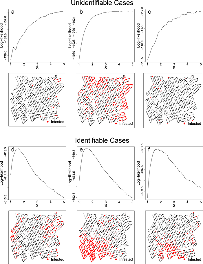
From the simulations, we identified two issues. First, for a small subset of simulated infestation patterns, it is difficult to identify the scale parameter S (Figure 3). The identification issue can be understood from the following example. Consider two infected houses on separate blocks and assume that the spatial components of the two locations are weakly correlated. This weak correlation can appear either due to a large value of the street barrier effect parameter S, or to a rapidly decreasing Matérn covariance function. The identification issue is easily overcome when a larger number samples is provided–but in the case of very scarce infestations, it is difficult to capture S (Figure 3ac). Rarely, we observe an oversaturated landscape, with few uninfested blocks, which also creates an unidentifiable pattern (Figure 3b). For more details on identification of S, see Appendix A. Secondly, the estimation of Matérn covariance parameters κ and ${\sigma }_u^2$ is not consistent. In Figure 4, each estimated covariance function is plotted and compared with the true covariance function. We can see that though $\widehat{\kappa }$ and ${\widehat{\sigma }}_u^2$ are biased, the estimated covariance function itself is remarkably close to the true function (Figure 4). Our main interest lies in capturing the function, rather than the individual covariance parameters, to create useful risk maps.

Figure 3:

Three unidentifiable and identifiable log-likelihoods and the corresponding simulated datasets. Unidentifiable landscapes were uncommon, (rates varied based on the true parameter values of κ and ${\sigma }_u^2$) and in most cases had scarce infestations (panels a and c). Occasionally, an unidentifiable landscape was oversaturated and also unidentifiable (panel b). For comparison, most simulated datasets were identifiable with clear maximums of the log-likelihoods (panels d, e, and f)

4. Data Results

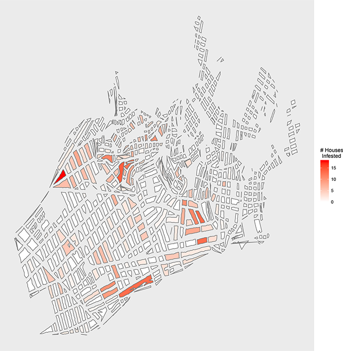
We apply the method to data collected during a vector control campaign in the district of Mariano Melgar in Arequipa in 2009. The district contains 12,069 houses, of which 586 were found to be infested with insect vectors (Figure 5). To fit the model to the dataset, we sample S over (1, 4) by increments of 0.1 and also estimate κ, ν, and β₀. We use the value of S that maximizes the log-likelihood of the model as our estimate, $\widehat{S}$, and the corresponding model parameters, $\widehat{\theta }$, and ${\widehat{\beta }}_0$.

Figure 5:

Map of the study region, the district of Mariano Melgar, Arequipa, Peru, which consists of 12,069 houses and 724 blocks. Color corresponds to number of known infested houses on the block. The map is made using a UTM projection.

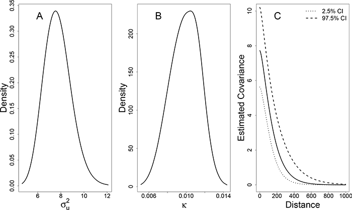
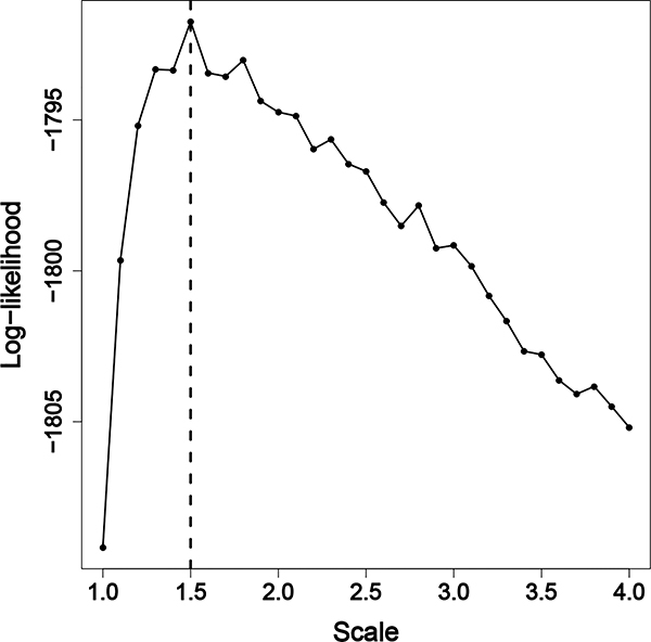
Using this approach, we find the the log-likelihood is maximized at S = 1.5. Our result indicates that streets are permeable barriers in the distribution of T. infestans, in agreement with previous studies (Barbu et al. (2013)). Our map contains blocks of varying sizes and shapes, and therefore our estimate, $\widehat{S}$, means the average minimum distance between houses on different blocks is increased 2.1 fold with a standard deviation of 0.5. This increase in average minimum distance is unique to our irregular map given the sizes and shapes of the city blocks. A scaled subsection of the map, incorporating this additional distance, can be seen in Figure 1B. Using this S, the covariance function is described using the estimates of κ = 0.009 with a 95% posterior credible interval of (0.007,0.013) and ${\sigma }_u^2=7.716$ with a 95% posterior credible interval of (5.492,10.047) (Figure 6). We estimate the model intercept, β₀ = −6.10 (0.41). Estimates of all parameters across values of S are summarized in Appendix B.

Figure 6:

Posterior distributions of estimated parameters when S = 1.5. A. Posterior distribution of ${\sigma }_u^2$ B. Posterior distribution of κ. C. Estimated posterior distribution of Matérn covariance, as a function of distance. For reference, when the map is scaled to S = 1.5, the average distance between nearest neighbors on the same block is 10.2 (sd = 5.5) and the average distance between nearest neighbors on different blocks is 62.4. (sd = 18.0)

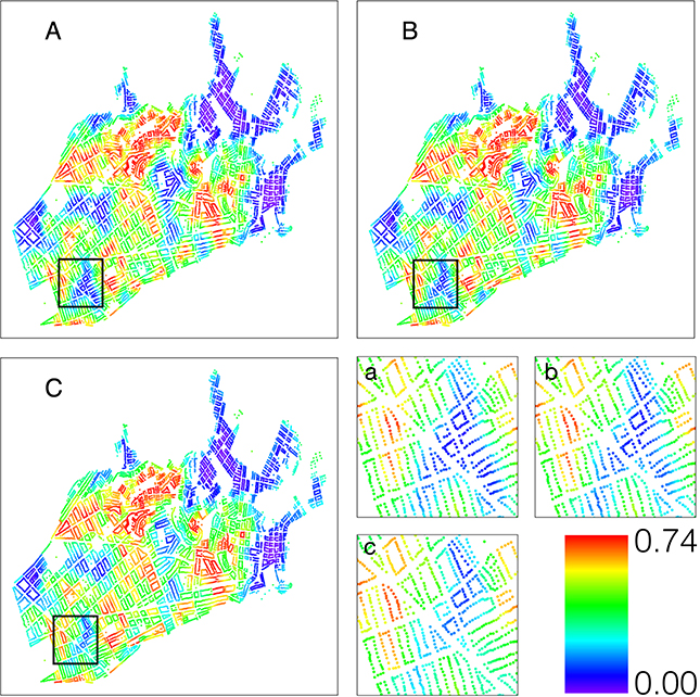
Using the scale of S = 1.5, we develop a risk map, representing the probability of infestation for each household (Figure 7). For comparison, we also present the risk map at S = 1, the true city map, and S = 3, additional widening of the barriers. Using this map, we can visualize the areas with elevated probability of infestation and compare the risk to the analysis without incorporating streets as barriers. Our estimates of the additional parameters, the covariance parameters θ, and the model intercept β₀, suggest there is significant spatial correlation between houses both within and between city blocks.

Figure 7:

Risk map of predicted probabilities of infestation using A) S = 1 (true map) B) S = 1.5 and C) S = 3. The last panel shows differences in risk between scales of the area enclosed in the black rectangle in more detail. The color scale ranges from 0.74 (red) to 0.00 (purple). The map is made using a UTM projection.

5. Discussion

We presented an approach to assess the significance of the urban landscape on the spatial distribution of disease vectors and quantify the effect of city streets in the distribution of the Chagas disease vector T. infestans in Arequipa, Peru. We estimated that streets add a distance of 50% to the true street width in the spatial distribution of vectors in the study region. Our estimate is qualitatively similar to Barbu et al. who estimated a fixed additional distance for each street regardless of the original width, however a direct comparison is difficult due to the difference in approaches (Barbu et al. (2013)).

Using the urban landscape and observed distribution of T. infestans in a portion of households, we created a risk map incorporating the city structure that can be used to guide searches over large areas of Arequipa for T. infestans. The methodology is easy to implement across large districts in Arequipa, and the risk maps are presented to control personnel in an easy to use application (Gutfraind et al. (in press)). By distorting the map and using Euclidean distance to define distance between points, we avoid complexities associated with using non-Euclidean distances (Curriero (2006)). The approach runs in just a few hours, or even less, depending on the size of the dataset and S used. On our dataset of 12,609 households, the process took 70 minutes when S = 1, 80 minutes when S = 1.5, and 90 minutes when S = 2. Overall, the time increases for larger values of S, but is much more affected by the size of the dataset. On smaller datasets, the approach can be completed in just a few minutes, even for large values of S.

Our model has limitations, both theoretically and in its interpretation. From our simulation studies, we observed specific unidentifiable datasets. We suspect that these parameter values occasionally generate simulated datasets where the pattern of infested houses is clustered such that the S is difficult to identify, including heavily clustering within a city block and lower total numbers of infested houses. From the likelihood plots (Figure 3), it is clear which datasets are unidentifiable, as they peak and then do not decrease as S increases. The unidentifiability of certain datasets is also a practical limitation, as scarce infestations are expected after control actions, and thus the barrier may not be identifiable.

The practical interpretation of our scale parameter, S, is complex when using irregular maps. While the distance between the center of each city block directly increases by S, the distance between points not at the center of each city block will increase by varying amounts depending on the size and shape of that particular block. Distortion of maps with irregularly shaped blocks may result in unintended changes, such as the alignment of blocks relative to each other. Incorporating multiple geographic barriers, such as streets and rivers, is difficult, if only one element is intended to be a barrier, or if they are barriers of different permeabilities.

In addition, our model assumes a constant scale factor for all barriers. In fact some streets, such as paved streets, may present more of a hindrance to insects than others. It would be quite difficult to incorporate covariates in the effects of barriers given within the framework presented here. Alternative methods have been developed to estimate complex spatial dependencies, which are arguably more statistically rigorous (Krivoruchko and Gribov (2004), Anders and Gudmund (2003), Sampson and Guttorp (1992), López-Quílez and Muñoz (2009)). However, the aim of our approach was to capture the spatial dependencies of the urban grid, while using fast and established statistical estimation software, so our methodology could be implemented to create risk maps in real time, and guide our field investigations. Hong developed a method that considers barriers such as streets as ‘sunken’ in relation to the remainder of the Gaussian field, rather than stretching the streets as we do here (Hong (2013)). Using grid methods similar to those we employ he estimated the degree of ‘sinkage’ of each barrier. His method would allow for greater flexibility to assess barriers of different types. In addition, his method is not affected by the irregularities of the specific urban grid. Hong et al also described a link between non-participation in vector control campaigns (from which these data are derived) and lower rates of infestation. We have not incorporated this association in our current analysis, which is another limitation to our approach. ‘Sinking’ the streets requires enormous and tedious manipulation of the triangulation used to approximate the Gaussian field, while stretching the streets is simple and easily incorporated into the existing R package, INLA. The ability to quickly incorporate our approach into existing software makes our method accessible to researchers across many disciplines for real-time risk map creation.

6. Conclusions

Risk maps are often used to develop epidemic predictions and intervention strategies. The observation of identifiable permeable barriers raises new potential targets for public health interventions in urban landscapes. For example, given our results, it may be more effective to inspect houses on the same city block as known infested houses rather than inspect houses within a set radius of them. We intend to use this modeling approach to guide inspections in Arequipa, Peru. As inspections are completed, we will update the model to reflect the latest observed infestations. The flexibility, generalizability, and computational efficiency make our approach a promising tool for real-time risk map creation.

Appendix A. Detailed simulation results

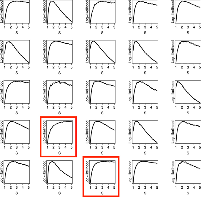
Our simulation studies suggest we need a minimum amount of observed information to identify the scale parameter. More research must be done to identify the requirements for identifiability of S. Our initial investigations suggest that the scale is identifiable when at least 2% of houses are infested, however this approximation also seems sensitive to the specific infestation pattern. The requirements may vary by the specific map and model used. In our testing, when the parameter is unidentifiable, the log-likelihood sharply increases near the true value but then does not decrease as the scale increases. It may be possible to identify specific patterns when these unidentifiable cases occur. As a general rule, we noticed unidentifiable likelihoods in cases with very low levels of infestation. Occasionally, we observed an unidentifiable likelihood when there was a high number of infested houses.

Table 4:

Simulation results with the variation in intercept β₀.

True values				Estimates
κ	${\mathit{\sigma }}_{\mathit{u}}^{\mathbf{2}}$	S	β0	$\widehat{\mathit{S}}$	${\widehat{\mathit{\beta }}}_{\mathbf{0}}$	Coverage (β0)	Identification
0.01	5	2.5	−3	2.68 (0.48)	−2.92 (0.35)	0.96	0.76
	10			2.69 (0.55)	−2.99 (0.49)	0.95	0.92
	25			2.65 (0.45)	−3.11 (0.79)	0.97	0.93
	50			2.65 (0.40)	−3.42 (1.21)	0.95	0.94
	100			2.67 (0.44)	−3.31 (l.86)	0.95	0.98
	200			2.64 (0.38)	−4.02 (3.24)	0.97	0.98

Table 5:

Simulation results with the variation in intercept κ.

True values				Estimates
κ	${\mathit{\sigma }}_{\mathit{u}}^{\mathbf{2}}$	S	β0	$\widehat{\mathit{S}}$	${\widehat{\mathit{\beta }}}_{\mathbf{0}}$	Coverage (β0)	Identification
0.001	5	1.5	−3	1.42 (0.52)	−2.35 (4.19)	0.93	0.69
0.002				1.52 (0.51)	−2.56 (1.34)	0.98	0.89
0.005				1.57 (0.35)	−3.11 (0.89)	1.00	0.95
0.01				1.64 (0.27)	−2.97 (0.53)	0.97	1.00
0.001	10	1.5	−3	1.70 (0.64)	−4.24 (6.78)	0.97	0.73
0.002				1.55 (0.45)	−2.63 (1.99)	1.00	0.93
0.005				1.61 (0.33)	−3.13 (1.26)	0.97	0.98
0.01				1.58 (0.19)	−3.16 (0.77)	0.96	1.00

Table 6:

Simulation results with the variation in intercept β₀.

True values				Estimates
κ	${\mathit{\sigma }}_{\mathit{u}}^{\mathbf{2}}$	S	β0	$\widehat{\mathit{S}}$	${\widehat{\mathit{\beta }}}_{\mathbf{0}}$	Coverage (β0)	Identification
0.005	5	2.5	−3	2.76 (0.48)	−2.91 (0.35)	0.96	0.76
			−4	2.64 (0.53)	−4.07 (0.46)	0.98	0.69
			−5	2.52 (0.58)	−5.06 (0.67)	0.92	0.66
			−6	2.12 (0.74)	−6.25 (l.17)	0.94	0.52

κ = 0.01, ${\sigma }_u^2$ = 5, S = 2.5 are fixed. The intercept β₀ varies from −6 to −3. The intercept plays a important role that decides the total number of infestations. A larger value of the intercept β₀ implies more infestations. Table 6 shows the simulation results with the variation in β₀. As β₀ decreases, the variation in the estimation of S increases and the identification rate decreases.

Figure 8:

Log-likelihood analysis across different scales, S. In most cases, S is clearly identifiable, but in some cases (red rectangles) it is not.

Appendix B. Additional Data Results

See Table 7 and Fig. 9

Figure 9:

Log-likelihood analysis across different scales, S. Likelihood is maximized at S = 1.5 indicating the model of best fit.

Table 7:

Results of grid sampling S on dataset, including estimates and standard deviations of θ₁, θ₂, and β₀. The log-likelihood is maximized when S = 1.5, and the bolded results are reported in the main text.

S	${\widehat{\mathit{\theta }}}_{\mathbf{1}}$	${\widehat{\mathit{\theta }}}_{\mathbf{2}}$	${\widehat{\mathit{\beta }}}_{\mathbf{0}}$	ll
1.0	2.06 (0.14)	−4.30 (0.14)	−6.14 (0.45)	−1809.18
1.1	2.08 (0.15)	−4.36 (0.17)	−6.16 (0.44)	−1799.65
1.2	2.13 (0.16)	−4.41 (0.20)	−6.15 (0.43)	−1795.19
1.3	2.19 (0.18)	−4.47 (0.21)	−6.13 (0.42)	−1793.33
1.4	2.36 (0.23)	−4.63 (0.21)	−6.10 (0.42)	−1793.35
1.5	2.35 (0.18)	−4.63 (0.17)	−6.10 (0.41)	−1791.74
1.6	2.45 (0.19)	−4.71 (0.19)	−6.07 (0.42)	−1793.44
1.7	2.49 (0.18)	−4.75 (0.19)	−6.06 (0.42)	−1793.56
1.8	2.54 (0.19)	−4.79 (0.19)	−6.06 (0.42)	−1793.02
1.9	2.61 (0.19)	−4.86 (0.18)	−6.04 (0.42)	−1794.38
2.0	2.66 (0.19)	−4.91 (0.18)	−6.03 (0.42)	−1794.74
2.1	2.71 (0.19)	−4.96 (0.18)	−6.03 (0.42)	−1794.87
2.2	2.77 (0.19)	−5.00 (0.17)	−6.02 (0.43)	−1795.97
2.3	2.82 (0.15)	−5.07 (0.15)	−6.00 (0.42)	−1795.65
2.4	2.85 (0.20)	−5.09 (0.18)	−6.01 (0.42)	−1796.46
2.5	2.88 (0.21)	−5.12 (0.19)	−6.01 (0.42)	−1796.70
2.6	2.95 (0.20)	−5.15 (0.18)	−6.01 (0.43)	−1797.74
2.7	3.00 (0.19)	−5.19 (0.17)	−6.00 (0.43)	−1798.51
2.8	3.02 (0.15)	−5.26 (0.15)	−5.99 (0.42)	−1797.84
2.9	3.06 (0.20)	−5.25 (0.18)	−6.00 (0.43)	−1799.25
3.0	3.11 (0.16)	−5.31 (0.15)	−5.99 (0.43)	−1799.15
3.1	3.11 (0.16)	−5.36 (0.16)	−5.97 (0.43)	−1799.84
3.2	3.16 (0.16)	−5.34 (0.15)	−5.98 (0.43)	−1800.82
3.3	3.21 (0.16)	−5.38 (0.15)	−5.98 (0.44)	−1801.66
3.4	3.24 (0.16)	−5.40 (0.15)	−5.97 (0.44)	−1802.66
3.5	3.30 (0.15)	−5.48 (0.14)	−5.97 (0.44)	−1802.78
3.6	3.31 (0.17)	−5.48 (0.16)	−5.97 (0.45)	−1803.63
3.7	3.37 (0.15)	−5.54 (0.14)	−5.96 (0.45)	−1804.08
3.8	3.35 (0.16)	−5.68 (0.19)	−5.93 (0.44)	−1803.83
3.9	3.39 (0.16)	−5.72 (0.19)	−5.93 (0.44)	−1804.50
4.0	3.40 (0.17)	−5.76 (0.19)	−5.92 (0.45)	−1805.19

References

- Adigun AB, Gajere EN, Oresanya O, Vounatsou P, 2015. Malaria risk in nigeria: Bayesian geostatistical modelling of 2010 malaria indicator survey data. Malaria journal 14 (1), 1. [DOI] [PMC free article] [PubMed] [Google Scholar]
- Anders L, Gudmund H, 2003. Spatial covariance modelling in a complex coastal domain by multidimensional scaling. Environmetrics 14 (3), 307–321. [Google Scholar]
- Barbu CM, Buttenheim AM, Pumahuanca M-LH, Calderón JEQ, Salazar R, Carrión M, Rospigliossi AC, Chavez FSM, Alvarez KO, del Carpio JC, et al. , 2014. Residual infestation and recolonization during urban Triatoma infestans bug control campaign, Peru. Emerging infectious diseases 20 (12), 2055. [DOI] [PMC free article] [PubMed] [Google Scholar]
- Barbu CM, Hong A, Manne JM, Small DS, Calderón JEQ, Sethuraman K, Quispe-Machaca V, Ancca-Juárez J, del Carpio JGC, Chavez FSM, et al. , 2013. The effects of city streets on an urban disease vector. PLoS Comput Biol. [DOI] [PMC free article] [PubMed] [Google Scholar]
- Bern C, 2015. Chagas’ disease. New England Journal of Medicine 373 (5), 456–466. [DOI] [PubMed] [Google Scholar]
- Besag J, 1975. Statistical analysis of non-lattice data. The statistician, 179–195. [Google Scholar]
- Blangiardo M, Cameletti M, Baio G, Rue H, 2013. Spatial and spatio-temporal models with r-inla. Spatial and spatio-temporal epidemiology 7, 39–55. [DOI] [PubMed] [Google Scholar]
- Bowman NM, Kawai V, Levy MZ, Del Carpio JGC, Cabrera L, Delgado F, Malaga F, Benzaquen EC, Pinedo VV, Steurer F, et al. , 2008. Chagas disease transmission in periurban communities of Arequipa, Peru. Clinical Infectious Diseases 46 (12), 1822–1828. [DOI] [PubMed] [Google Scholar]
- Brooker S, 2007. Spatial epidemiology of human schistosomiasis in Africa: risk models, transmission dynamics and control. Transactions of The Royal Society of Tropical Medicine and Hygiene 101 (1), 1–8. [DOI] [PMC free article] [PubMed] [Google Scholar]
- Curriero FC, November 2006. On the use of non-euclidean distance measures in geostatistics. Mathematical Geology 38 (8), 907–926. [Google Scholar]
- Delgado S, Ernst KC, Pumahuanca MLH, Yool SR, Comrie AC, Sterling CR, Gilman RH, Náquira C, Levy MZ, 2013. A country bug in the city: urban infestation by the chagas disease vector triatoma infestans in arequipa, peru. International journal of health geographics 12 (1), 1. [DOI] [PMC free article] [PubMed] [Google Scholar]
- Dias JCP, Silveira AC, Schofield CJ, 2002. The impact of chagas disease control in latin america: a review. Memórias do Instituto Oswaldo Cruz 97 (5), 603–612. [DOI] [PubMed] [Google Scholar]
- Diggle PJ, Ribeiro PJ Jr, Christensen OF, 2003. An introduction to model-based geostatistics In: Spatial statistics and computational methods. Springer, pp. 43–86. [Google Scholar]
- Gutfraind A, Peterson JK, Rose EB, Arevalo-Nieto C, Sheen J, CondoriLuna GF, Tankasala N, Castillo-Neyra R, Condori C, Anand P, NaquiraVelarde C, Levy MZ, in press Integrating evidence, models and maps to enhance chagas disease vector surveillance. PLOS Neglected Tropical Diseases. [DOI] [PMC free article] [PubMed] [Google Scholar]
- Haley RW, 2012. Controlling urban epidemics of west nile virus infection. JAMA 308 (13), 1325–1326. [DOI] [PubMed] [Google Scholar]
- Hong AE, 2013. Gaussian markov random field models for surveillance error and geographic boundaries. Ph.D. thesis, University of Pennsylvania. [Google Scholar]
- Jaya IGNM, Abdullah AS, Hermawan E, Ruchjana BN, 2016. Bayesian spatial modeling and mapping of Dengue fever: A case study of Dengue fever in the city of Bandung, Indonesia. International Journal of Applied Mathematics and Statistics™ 54 (3), 94–103. [Google Scholar]
- Knudsen AB, Slooff R, 1992. Vector-borne disease problems in rapid urbanization: new approaches to vector control. Bulletin of the World Health Organization 70 (1), 1. [PMC free article] [PubMed] [Google Scholar]
- Krainski E, Lindgren F, 2013. The R-INLA tutorial: SPDE models. [Google Scholar]
- Krivoruchko K, Gribov A, 2004. Geostatistical interpolation and simulation in the presence of barriers In: Sanchez-Vila X, Carrera J, Gómez-Hernández JJ (Eds.), geoENV IV — Geostatistics for Environmental Applications. Springer; Netherlands, Dordrecht, pp. 331–342. [Google Scholar]
- LaDeau SL, Allan BF, Leisnham PT, Levy MZ, 2015. The ecological foundations of transmission potential and vector-borne disease in urban landscapes. Functional ecology 29 (7), 889–901. [DOI] [PMC free article] [PubMed] [Google Scholar]
- Levy MZ, Bowman NM, Kawai V, Waller LA, del Carpio JGC, Benzaquen EC, Gilman RH, Bern C, 2006. Periurban Trypanosoma cruzi–infected Triatoma infestans, Arequipa, Peru. Emerging infectious diseases 12 (9), 1345. [DOI] [PMC free article] [PubMed] [Google Scholar]
- Lindgren F, Rue H, Lindström J, 2011. An explicit link between Gaussian fields and Gaussian Markov random fields: the stochastic partial differential equation approach. Journal of the Royal Statistical Society: Series B (Statistical Methodology) 73 (4), 423–498. [Google Scholar]
- López-Quílez A, Muñoz F, 2009. Geostatistical computing of acoustic maps in the presence of barriers. Mathematical and Computer Modelling 50 (5), 929–938, mathematical Models in Medicine & Engineering. [Google Scholar]
- Oluwole AS, Ekpo UF, Karagiannis-Voules D-A, Abe EM, Olamiju FO, Isiyaku S, Okoronkwo C, Saka Y, Nebe OJ, Braide EI, et al. , 2015. Bayesian geostatistical model-based estimates of soil-transmitted helminth infection in nigeria, including annual deworming requirements. PLoS Negl Trop Dis 9 (4), e0003740. [DOI] [PMC free article] [PubMed] [Google Scholar]
- Rossi RE, Mulla DJ, Journel AG, Franz EH, 1992. Geostatistical tools for modeling and interpreting ecological spatial dependence. Ecological Monographs 62 (2), 277–314. [Google Scholar]
- Rue H, Held L, 2005. Gaussian Markov random fields: theory and applications. CRC Press. [Google Scholar]
- Rue H, Martino S, Chopin N, 2009. Approximate bayesian inference for latent gaussian models by using integrated nested laplace approximations. Journal of the royal statistical society: Series b (statistical methodology) 71 (2), 319–392. [Google Scholar]
- Rue H, Martino S, Lindgren F, Simpson D, Riebler A, Krainski ET, 2014. INLA: Functions which allow to perform full Bayesian analysis of latent Gaussian models using integrated nested Laplace approximaxion. R package version 0.0–1389624686. [Google Scholar]
- Sampson PD, Guttorp P, 1992. Nonparametric estimation of nonstationary spatial covariance structure. Journal of the American Statistical Association 87 (417), 108–119. [Google Scholar]
- Sikka V, Chattu VK, Popli RK, Galwankar SC, Kelkar D, Sawicki SG, Stawicki SP, Papadimos TJ, 2016. The emergence of zika virus as a global health security threat: A review and a consensus statement of the indusem joint working group (jwg). Journal of global infectious diseases 8 (1), 3. [DOI] [PMC free article] [PubMed] [Google Scholar]
- Weaver SC, 2013. Urbanization and geographic expansion of zoonotic arboviral diseases: mechanisms and potential strategies for prevention. Trends in microbiology 21 (8), 360–363. [DOI] [PMC free article] [PubMed] [Google Scholar]
- Whittle P, 1954. On stationary processes in the plane. Biometrika, 434–449. [Google Scholar]
- Whittle P, 1963. Stochastic-processes in several dimensions. Bulletin of the International Statistical Institute 40 (2), 974–994. [Google Scholar]
Associated Data
This section collects any data citations, data availability statements, or supplementary materials included in this article.