Systematic Dose-Response of Environmental Epidemiologic Studies: Dose and Response Pre-Analysis

Abstract

Meta-analysis approaches can be used to assess the human risks due to exposure to environmental chemicals when there are numerous high-quality epidemiologic studies of priority outcomes in a database. However, methodological issues related to how different studies report effect measures and incorporate exposure into their analyses arise that complicate the pooled analysis of multiple studies. As such, there are “pre-analysis” steps that are often necessary to prepare summary data reported in epidemiologic studies for dose-response analysis. This paper uses epidemiologic studies of arsenic-induced health effects as a case example and addresses the issues surrounding the estimation of mean doses from censored dose- or exposure-intervals reported in the literature (e.g., estimation of mean doses from high exposures that are only reported as an open-ended interval), calculation of a common dose metric for use in a dose-response meta-analysis (one that takes into consideration inter-individual variability), and calculation of response “effective counts” that inherently account for confounders. The methods herein may be generalizable to 1) the analysis of other environmental contaminants with a suitable database of epidemiologic studies, and 2) any meta-analytic approach used to pool information across studies. A second companion paper detailing the use of “pre-analyzed” data in a hierarchical Bayesian dose-response model and techniques for extrapolating risks to target populations follows.

1. Introduction

While dose-response analyses for the purpose of human health risk assessment have typically been conducted by applying dose-response modeling techniques to a single, perhaps “best” animal toxicological data set, data from epidemiologic studies have been used less frequently. As of 2007, approximately 8% (44) of the 545 chemical assessments in the IRIS database were identified as using human data in the derivation of toxicity values (Persad and Cooper 2008) and several more recent assessments (ethylene oxide, hydrogen cyanide, Libby amphibole asbestos, 2,3,7,8-tetrachlodibenzo-p-dioxin, tetrachloroethylene and trichloroethylene) make use of epidemiologic data for quantitative purposes (U.S. EPA 2019). The use of epidemiologic data is preferable over the use of animal data because it avoids issues related to interspecies extrapolation to account for differences in toxicokinetics and toxicodynamics (U.S. EPA 2005). However, when using epidemiologic data, there is often a need to integrate information from a variety of sources. Meta-analysis explicitly involves simultaneous modeling of studies, yielding pooled estimates, in order to leverage information from multiple studies, possibly further decreasing uncertainties surrounding the use of individual studies (i.e., human variability, etc.).

However, it is often the case that risk assessors are limited to information they can obtain from the peer-reviewed literature and overwhelmingly this results in only summary data being available. As such, the following methods should prove valuable for increasing the role of epidemiologic studies in quantitative dose-response analyses in human health risk assessment.

This is the first in a series of two papers that will address the use of epidemiologic studies for dose-response analyses for the purpose of identifying target population risks in a human health risk assessment. The approaches outlined in these two papers expand upon previous methods applied by EPA in IRIS assessments for the evaluation of epidemiologic data (U.S. EPA 2017) in several respects. An important feature of this approach is that the studies suitable for combination in our dose-response meta-analysis (DRMA) can be either cohort studies or case-control studies. In particular, we want to emphasize and illustrate what we consider to be important, and potentially novel, components of such an analysis through a case study of inorganic arsenic drinking water exposure and bladder cancer morbidity.

Figure 1 displays the overall flow of the DRMA analysis. In this first manuscript, we address issues that typically arise when dealing with summarized (e.g., published) analyses, shown in blue in Figure 1. We categorize these as “pre-analysis” steps, in the sense that they prepare the data so that they are amenable to dose-response modeling and characterize uncertainties associated with the data presentations available to the modeler. These steps are preliminary steps that allow for a systematic dose-response analysis that combines data from multiple studies.

Figure 1: Analysis Flow Chart.

The analyses covered in this paper are highlighted in blue whereas the analyses highlighted in orange and green are covered in the second paper of this series (Allen et al., 2020)

The subsequent paper will focus on the choice of models, the statistical rationale for their use, and how they can be suitable for studies of different types (cohort and case-control). Details of a Bayesian DRMA will be provided, including important derivations that allow or facilitate analysis (orange section of Figure 1). That paper will also demonstrate how the results of the dose-response modeling will be extrapolated to a target population of interest using lifetable analysis approaches (shown in green in Figure 1).

All of the steps illustrated on Figure 1 will be performed in the context of epidemiologic studies relating arsenic exposure (through drinking water) to bladder cancer incidence. The specific studies included in this analysis are discussed briefly in the following section. Subsequent sections of this manuscript will address dose estimation for interval-censored data, including the important consideration of uncertainty in dose metric values, and the use of reported numbers of cases to calculate effective counts that reflect adjustments for potential confounders. This manuscript ends with a discussion of pertinent issues and of the linkage to the DRMA implementation detailed in the second paper in this series.

2. Methods and Case-Study Results

2.1. Case-Study: Epidemiologic Studies of Arsenic and Bladder Cancer

The case study underlying the methodologies discussed here is based on published reports that link arsenic exposure to bladder cancer morbidity. Multiple health agencies have concluded that the relationship between arsenic exposure and bladder cancer is causal (NRC, 2013; ATSDR, 2016; ATSDR 2007; NTP, 2016; IARC 2012; WHO 2011a,b); we take that as a given for our analyses.

Multiple bladder cancer studies considered to have sufficient information to support a dose-response analysis will be used in the actual dose-response portion of this analysis (see second paper, Allen et al. 2020). It should be noted that these studies do not necessarily represent the final set of epidemiologic studies that might be chosen for a formal human health risk assessment. For the purposes of this paper (i.e., demonstration of the pre-analysis steps), we have focused on only two such studies, a cohort study (Chen et al. 2010) and a case-control study (Meliker et al. 2010), as the pre-analysis steps differ slightly given different study designs. The second paper (Allen et al., 2020) describing the Bayesian DRMA methods will provide more details on other studies included in the analysis.

In this case, the two studies selected here to demonstrate the dose and response conversions each had three or more exposure groups defined in the published reports, including the “referent” group (i.e., the group to which other groups are compared in order to calculate the relative risk or odds ratio). It is worth noting, however, that in a DRMA context, there is no need to exclude studies with only two exposure groups, nor would inclusion of two-group studies necessarily limit the “complexity” of the models applied. The fact that several studies are modeled together provides data at more than two exposure levels and allows for more inclusiveness with respect to study selection and dose-response model forms.

2.2. Pre-analyses for the Estimation of a Common Dose

One of the novel aspects that distinguishes the current approach from other meta-analyses of epidemiologic data, such as the recently published arsenic meta-analyses for bladder and lung cancer by Lynch et al. (2017a; b) and for cardiovascular diseases by Moon et al. (2017), is the conversion of route-specific (e.g., oral) exposure metrics commonly used in epidemiologic risk assessments (e.g., drinking water concentrations, measures of cumulative exposure) to a common dose metric (e.g., total daily oral intake) that is presumed to be more closely related to the responses for the health effect in question. Conversion of disparate exposure metrics to a single unified dose metric removes the restriction of choosing a “best” exposure metric and thus allows for a larger set of studies to be used in the DRMA. When drinking water is the primary exposure route, Baris et al. (2016) emphasized the importance of incorporating estimates of water intake for the reliable discernment of dose-response relationships, particularly for low to moderately exposed populations. As examples, the cohort study (Chen et al. 2010) and the case-control study (Meliker et al. 2010) vary with respect to the units in which exposure or dose were presented: ug/L-year and ug/day, respectively. As such, a primary requirement for the pre-analysis is the specification of a common unit of dose and conversion of all study doses to that scale. The units of interest for this analysis were average daily μg inorganic arsenic (iAs) intake per kg bodyweight (average daily μg/kg).

In practice, we combined the requirement for a common dose metric with the need to estimate a mean dose for each group that is merely represented by a range of dose values in the actual studies. In most published reports, groups are commonly defined by the range of exposures experienced by the individuals (or person-years) in the group; they are “interval censored” with respect to exposure. Thus, we first computed means (in units as given in the published papers) and then applied the conversions to those means. This process is summarized in Figure 2, which shows that accounting for uncertainties in the estimation of the means or of the conversions is an integral part of this exercise. For the mean estimation, the process is summarized as follows.

Figure 2: Dose Pre-Analysis and Uncertainty Flow Chart in Relation to “Best,” Low-end, and High-end Dose Sets.

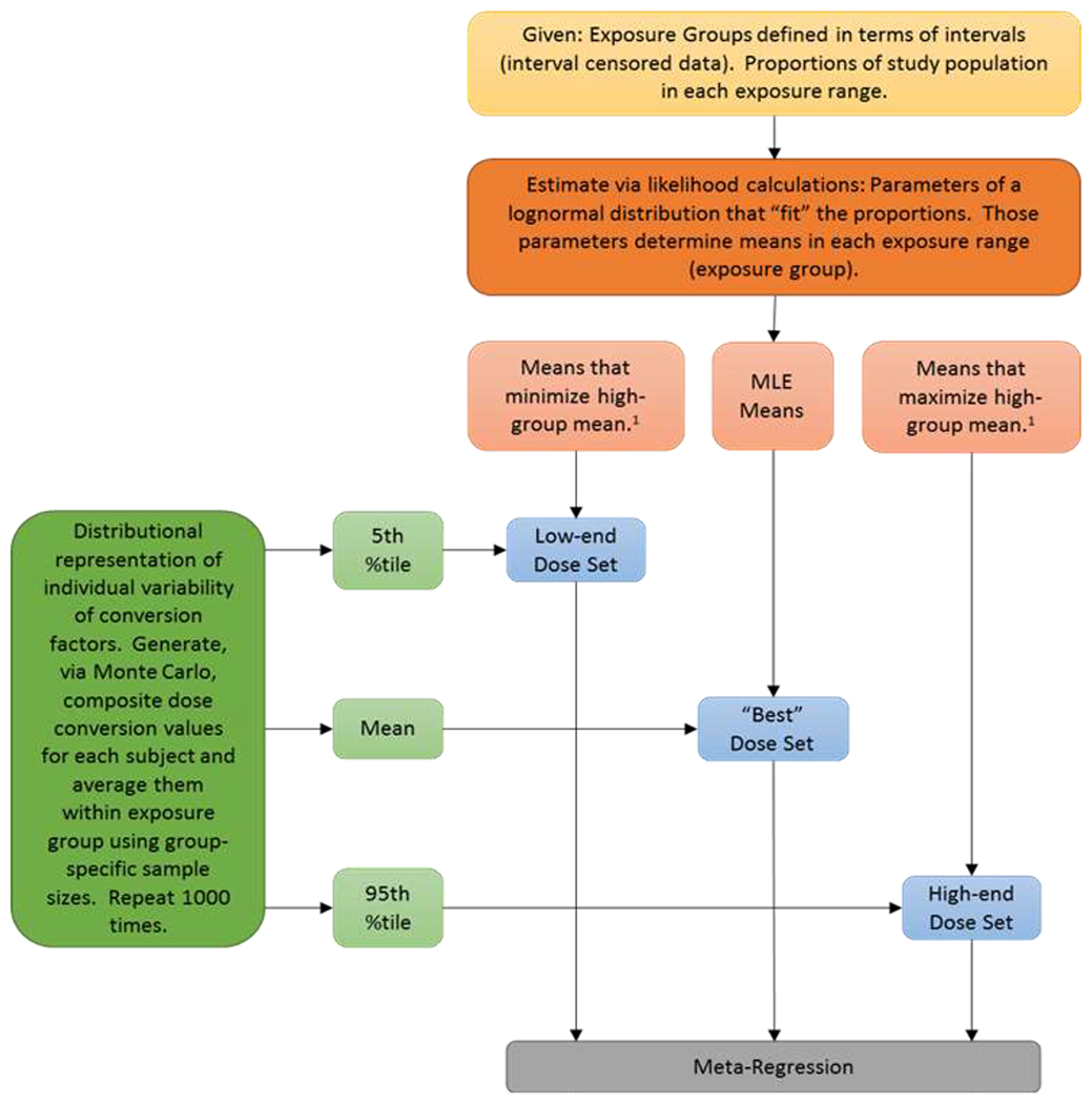
¹ High group means minimized or maximized subject to constraint that −2 × (LL – MLL) ≤ 2.706 (a 95% bound on the high-group mean). LL is the log-likelihood for the lognormal distribution for the candidate parameter vector; MLL is the maximum log-likelihood. When a published study reports the mean or median values for each group, those values are used directly as the group-specific dose values, with no lognormal fitting. ² The terminology “low-end,” “high-end,” and “best” estimates are used to avoid confusing the values with credible (or confidence) interval bounds having a specific numerical value (e.g., 95%). Combining the log-likelihood bounds for group-specific means, with percentiles from the Monte Carlo analysis does not allow determination that the bounding estimates have any identifiable associated “confidence level.” They do, however produce reasonable semi-quantitative limits on how uncertain the resulting estimates are.

2.3. Group Means and Uncertainty

Suppose that a study has G exposure groups defined as (c₀, c₁), (c₁, c₂), … , (c_G−1, c_G); c₀ may equal 0 and c_G may equal ∞. Let τ, with elements τ_g, be the vector of observed proportions of individuals in groups g = 1, …, G. As discussed below, for a case-control study, only the control counts were used to define the τ values; otherwise all individuals were used to define τ.

We assume that individual exposures follow a lognormal distribution with parameters μ and σ (respectively, the mean and standard deviation of natural logarithms of exposure); the same assumption was made by Moon et al. (2017) in their analysis of arsenic risks. We estimate these parameters by maximum likelihood (ML), maximizing the following log-likelihood expression appropriate for the censored data:

$$\mathit{log}-\text{likelihood}=N\cdot {\sum }_{g=1}^G{\tau }_g\cdot \mathit{ln}(\phi (\mathit{ln}(c_g)\mid \mu ,\sigma )-\phi (\mathit{ln}(c_{g-1})\mid \mu ,\sigma ))$$

where N is the total number of observations under consideration and φ(x | μ, σ) is the cumulative distribution function for the Normal distribution with mean μ and standard deviation σ. Let μ’ and σ’ be the ML estimates (MLEs) given τ and the values of c_g (g = 0, …, G). A simple likelihood maximization routine, implemented with an Excel spreadsheet (see Supplemental Material), was used to estimate μ’ and σ’.

Given μ’ and σ’, the mean within a given exposure interval (c_g, c_g+1) is given by

$$\text{mean}(g)=e^{\left(\mu \prime +\frac{\sigma {\prime }^2}{2}\right)}\times \frac{\theta (U_1(g)-\sigma \prime )-\theta (U_0(g)-\sigma \prime )}{\theta (U_1(g))-\theta (U_0(g))},$$ Eq. 1

where $U_1(g)=\frac{(\mathit{ln}(c_{g+1})-\mu \prime )}{\sigma \prime }$, $U_0(g)=\frac{(\mathit{ln}(c_g)-\mu \prime )}{\sigma \prime }$, and θ() is the cumulative distribution function for the standard normal distribution (Söderlind 2013).

In addition to the maximum likelihood estimate of an exposure for each dose group, we have computed what are referred to as “low-end” and “high-end” exposure estimates. Those estimates were based on profile likelihood bounds for the mean exposure for individuals in the high-exposure group. First, we computed the maximized log-likelihood (MLL) (the log-likelihood associated with MLEs of the parameters μ and σ). Then the mean value for the high-group was maximized by modifying μ and σ subject to the constraint that

$$-2\times (\mathit{LL}-\mathit{MLL})\le 2.706$$ Eq. 2

where LL is the log-likelihood associated with the modified μ and σ. This is a chi-squared-based (1 degree of freedom) 95% confidence upper bound on the high-group mean. The same procedure was followed to determine a 95% confidence lower bound on the high-group mean by minimizing the mean value for the high group under the same constraint (Eq. 2). Supplemental Files S3 and S4 demonstrate fully these calculations.

Note that we are only specifically maximizing (or minimizing) the mean for the highest exposure group. In some instances, this may result in a change in the estimated mean for other groups (primarily the lowest exposure group) when the modified μ and σ are input into Eq. 1. We have opted for this procedure for two primary reasons. First, the highest exposure group is almost always the one that is most uncertain, often presented as an open-ended interval. The mean for that group is not easily nor consistently estimated by techniques that can be applied to the other exposure groups (e.g., by taking the midpoint of the interval). Second, the dose and response observations for the highest exposure group often have a large impact on dose-response model estimation. Especially for the slope parameters in a model, the positioning of the highest dose-response pair can be very influential. Thus, our procedure focuses on that influential observation and derives bounds specifically tailored to determine the full range of possible values for exposure consistent with the data (and our assumption of lognormality of exposures over the studied population) for that observation. Additional discussion about the choice of the lognormal distribution is provided in the Discussion section.

2.4. Dose Conversions and Uncertainty

As discussed above in Section 2.2, estimation of a common dose metric (as opposed to exposure metric) for all studies is imperative in order to account for the effect of dose on the estimated response. However, epidemiologic studies often use different, but related, exposure- or dose-metrics such as exposure concentration, cumulative exposure, and even biomarkers of exposure such as internal tissue concentrations or urinary concentrations of the chemical of interest. In this specific case-report, if the data presented in all the published studies had been in the units of interest (daily average μg/kg), no conversion would be necessary and DRMA could be performed with the study-reported data. However, that was not the case for any of the studies under consideration here, nor would it be in general practice.

First, all of the factors required to convert to μg/kg were identified. As an example, consider the Chen et al. (2010) study of bladder cancer. The tabulation of results reported in that study reported cumulative drinking water exposures, in (μg iAs/L drinking water) · years. The conversion from cumulative exposures to average daily dose (μg/kg) was carried out as follows:

$$\text{dose}=\mathit{DI}+f\times (\mathit{WCR}\times \mathit{WE})+(1-f)\times (\mathit{WCR}\times \mathit{LE})$$ Eq.3

where the terms in that expression are: DI = dietary intake (average daily μg/kg); f = fraction of time (over lifetime up through the study) spent consuming well water (unitless); WCR = water consumption rate (L/kg); WE = well water concentration (μg/L); and LE = low-end water concentration (μg/L). The variable f was calculated as the ratio of the assumed average duration of well exposure (ADWE), generally the reported duration of drinking well water (RDWE; yr), to the average age at diagnosis (AAD; yr). It was assumed that when drinking non-well water, the subjects consumed water with the low-end water concentration. The parameter WE was derived separately for each group by dividing the reported cumulative exposure (CE; μg/L · yr) for that group by the $\mathrm{RDWE}:\mathit{WE}=\frac{\mathit{CE}}{\mathit{RDWE}}$. The values used in Eq. 3 above ideally would come from study-specific data reported in the study of interest, but could also be drawn from other suitable sources (see Table 1 for specific examples for the Chen et al. (2010) dose conversions). For instance, for Chen et al. (2010), the ADWE, AAD, and RDWE variables were drawn from the Chen et al. (2010) study or papers detailing analyses of the same cohort (Hsieh et al. 2008) (Table 1). Information on WCR and DI, however, was drawn from the Taiwanese Exposure Factor Handbook (TDOH 2007).

Table 1:

Variables Used in the Dose Conversions for the Chen et al. (2010) Study, Including Data Sources

Variable (units)	Mean	SD	Justification for Value and Data Source
ADWE – Assumed average duration of well exposure (yrs)	42	--	Reported average duration of drinking well water was 42 years for this cohort (Chiou et al. 2001; Hsieh et al. 2008)
AAD – Average age at diagnosis (yrs)	65	--	Midpoint between average age at baseline and average age after follow-up; estimated from data reported by Chen et al. (2010)
LE – Low water exposure (μg/L)	5	15	Out of study low (LE) exposures are assumed to be below 10 μ/L, but because of higher 50 μ/L MEL in Taiwan (Guo and Valberg 1997), allowed higher variability (values above 50 would be rare).
WCR – Water consumption rate (ml/kg-day)	34.5	23.2	Natural scale mean and std were computed from log-scale mean and SD values estimated for lognormal distribution that matches 5th and 95th percentiles of Taiwanese Exposure Handbook (TDOH 2007).
DI – Dietary intake (μg/kg-day)	0.65	0.33	Based on an analysis of Taiwanese eating habits (TDOH 2007). Absorption fraction for foods was assumed to be 0.80. Absorption fraction for cooking water was assumed to be 1.0.
RDWE – Reported average duration of well exposure (yrs)	42	3.33	Reported average duration of drinking well water was 42 years for this cohort (Chiou et al. 2001; Hsieh et al. 2008)

Importantly, the factors affecting conversion were not treated as single values. Rather, a distribution was assumed over the individuals in the study and the specific type of distribution was allowed to differ for different variables. For instance, lognormal distributions were assumed for DI, WCR, RDWE, and LE, whereas a beta distribution was used for the f variable. Those distributions were expressed in terms of inter-individual variability and were based on knowledge of the population from which the study participants were drawn (e.g., exposure factors handbook values or study-specific data). Thus, when converting the group-specific mean cumulative values to group-specific mean μg/kg values, we sampled from the relevant distributions (in the example above, for DI, f, WCR, LE, and RDWE) and computed the resulting conversion for each individual in the exposure group in question (in cases where the n per dose group was greater than 1000, the average was computed using 1000 samples to ease computational burden). Then we averaged over all the individuals in the group, to come up with a group mean conversion (see Table 2). A Monte Carlo (MC) simulation was conducted in which this process was repeated 1,000 times to derive a distribution of averaged dose values. The median as well as the 2.5^th and 97.5^th percentiles were pulled from the MC results to characterize the best, low-end and high-end dose values (Figure 2; Tables 3 and 4). As expected, given the methods used to estimate dose group means (see Section 2.3), the resulting differences in the high exposure group mean were substantial when using either the “MLE”, “high”, or “low” dose scenarios whereas the low exposure group mean distribution were not (see Table 4, Figure 3).

Table 2:

Example of Dose Calculations – Converting Reported cumulative exposure (μg/L-year) in Chen et al. (2010) to daily intakes (μg/kg-day) for one dose group

Variable	DI	f	WCR	RDWE	LE	WE – MLE2	MLE Dose	WE - Low	Low Dose	WE - High	High Dose
Mean1	0.65	0.630769	0.0345	42	5
SD	0.333333	--	0.02319	3.333333	15
Distribution	LogNormal	Beta	LogNormal	LogNormal	LogNormal
Study Participant
1	0.469875	0.739176	0.020187	47.73289	0.955895	3.29	0.524063	3.35	0.524879	3.24	0.523245
2	0.448139	0.548615	0.019016	37.84907	0.088638	4.15	0.492239	4.22	0.492959	4.09	0.491518
3	0.443911	0.525224	0.089145	37.46044	0.775256	4.20	0.673251	4.27	0.676512	4.13	0.669982
4	0.239939	0.716066	0.034483	39.79564	0.316072	3.95	0.340594	4.02	0.342213	3.89	0.338971
5	0.729251	0.762123	0.011225	44.53952	0.129244	3.53	0.759797	3.59	0.760298	3.47	0.759294
6	0.328373	0.566265	0.024349	39.57211	4.685345	3.97	0.432639	4.04	0.433548	3.91	0.431728
7	1.290163	0.444601	0.024441	46.76837	1.800928	3.36	1.351143	3.42	1.351749	3.31	1.350535
8	1.112427	0.459657	0.033277	38.34288	7.113424	4.10	1.30306	4.17	1.304101	4.03	1.302017
9	0.35606	0.639259	0.06128	38.18047	0.947065	4.12	0.538323	4.19	0.541001	4.05	0.53564
10	0.74094	0.775479	0.047677	43.18117	0.405901	3.64	0.879915	3.70	0.882149	3.58	0.877675
--	--	--	--	--	--	--	--	--	--	--	--
10003	0.540283	0.868618	0.026601	45.62604	33.13435	3.45	0.735713	3.50	0.737035	3.39	0.734389
Average							0.784552		0.785761		0.78334

DI = dietary exposure (average daily μg/kg), f = ratio of assumed average duration of well exposure (ADWE, yr) and average age at diagnosis (AAD, yr), WCR = water consumption rate (ml/kg-day), RDWE = reported duration of we exposure (yr), LE = low exposure (μg/L)

¹See Table 1 for variable values and justifications

²WE (well exposure, μg/L) = CE (cumulative exposure; μg/L-years) /RDWE (yr); CE for this table is the “Best” cumulative exposure calculated for the referent group: 157 μg/L-years (see Table 4)

³Assumed distributions with associated means and standard deviations are sampled a number of times equal to the dose-specific Ns, for doses with N > 1000, 1000 samples are taken to ease computational burden

Table 3:

Results of the Monte Carlo Simulation Analysis to Calculate MLE, Low, and High Dose Estimates for Chen et al. (2010)

Cumulative iAs water exposure, μg/L · years	Dose Scenarios	Mean	Standard Deviation	0%	1%	5%	10%	25%	50%	75%	90%	95%	99%	100%
< 400	High	0.802	0.014	0.764	0.775	0.781	0.786	0.793	0.802	0.811	0.821	0.826	0.837	0.852
	Low	0.805	0.014	0.767	0.778	0.784	0.789	0.796	0.804	0.814	0.823	0.828	0.840	0.854
	MLE	0.804	0.014	0.765	0.776	0.783	0.787	0.794	0.803	0.813	0.822	0.827	0.838	0.853
400–1,000	High	1.052	0.016	1.008	1.017	1.027	1.033	1.042	1.051	1.062	1.072	1.078	1.091	1.111
	Low	1.052	0.016	1.008	1.017	1.027	1.033	1.042	1.051	1.062	1.073	1.078	1.091	1.111
	MLE	1.052	0.016	1.008	1.017	1.027	1.033	1.042	1.051	1.062	1.072	1.078	1.091	1.111
1,000–5,000	High	1.893	0.032	1.781	1.818	1.839	1.852	1.872	1.893	1.915	1.935	1.945	1.969	1.995
	Low	1.887	0.032	1.776	1.812	1.834	1.847	1.866	1.888	1.909	1.929	1.940	1.963	1.989
	MLE	1.890	0.032	1.779	1.815	1.837	1.849	1.869	1.891	1.912	1.932	1.943	1.966	1.992
5,000–10,000	High	4.245	0.123	3.880	3.961	4.032	4.086	4.164	4.245	4.329	4.397	4.443	4.526	4.677
	Low	4.238	0.123	3.874	3.955	4.026	4.080	4.157	4.239	4.322	4.390	4.436	4.519	4.669
	MLE	4.241	0.123	3.877	3.958	4.029	4.083	4.161	4.242	4.326	4.393	4.439	4.523	4.673
>10,000	High	20.487	0.597	18.322	19.152	19.481	19.720	20.083	20.478	20.867	21.292	21.477	21.858	22.285
	Low	18.687	0.543	16.718	17.475	17.774	17.992	18.320	18.679	19.032	19.420	19.588	19.935	20.325
	MLE	19.555	0.569	17.492	18.284	18.598	18.826	19.171	19.547	19.917	20.323	20.499	20.863	21.271

Table 4:

Final Dose Conversion Results for MLE, High, and Low Daily Lifetime Dose Estimates for Chen et al. (2010)

Cumulative iAs water exposure, μg/L · years	Cumulative Exposure (μg/L·years)			Lifetime Average Daily Dose (μg/kg)
	“Best”1	Low	High	“Best”	Low	High
< 400	157	160	155	0.80	0.78	0.83
400–1,000	657	657	657	1.05	1.03	1.08
1,000–5,000	2343	2337	2349	1.89	1.83	1.95
5,000–10,000	7048	7041	7055	4.24	4.03	4.44
>10,000	37873	36127	39746	19.56	17.77	21.48

¹Maximum Likelihood estimate

Figure 3: Effect of Group Mean Estimations (MLE, High, Low) on Final Distribution of Daily Intake Dose Estimates for the Lowest and Highest Exposure Group in Chen et al. (2010).

Plot represents the distribution of the percentiles of the dose-estimation MCMC analysis for the low- and high-exposure groups. Frequencies were calculated in Excel using the “Frequency” function and user-defined bin values.

Other items to note include the fact that we have included dietary exposure in all the conversions. Thus, our dose estimates represent total inorganic arsenic intake from all oral routes, not necessarily just exposure from drinking water. Our approach explicitly considers the sample sizes in each exposure group; by averaging over the number of individuals in each group, we have automatically considered that groups with more observations will be less uncertain (about the mean group-specific conversions) than groups with fewer observations.

Finally, note that each study, possibly reporting different exposure summaries, is handled differently depending on the reported units. For example, the Meliker et al. (2010) study used daily arsenic exposure (in units of μg/day) as the dose metric rather than cumulative exposure in units of (μg iAs/L drinking water) · years as did Chen et al. (2010). Thus, the conversion to average daily μg/kg (dose) was carried out for the Meliker et al. (2010) study as follows:

$$\text{dose}=\mathit{DI}+f\times \left(\frac{\mathit{WE}}{\mathit{BW}}\right)+(1-f)\times (\mathit{WCR}\times \mathit{LE})$$ Eq.4

where the terms in that expression are as above with the addition of BW = body weight (kg). The variable f was estimated as described above, but in the case of the Meliker et al. (2010) study, the parameter WE was derived separately for each group by dividing the reported daily exposure (μg/day) for that group by a BW value selected from a normal distribution centered at the average bodyweight from the EPA Exposure Factors handbook (2011).

All dose conversions were computed via Excel, using the MC simulation add-in Yasai (www.yasai.rutgers.edu). While other software programs or languages (i.e., R or Python) are more powerful in some regards and could be used to implement the dose-conversions, Excel was chosen for its ubiquity of use and because Excel workbooks are useful for organizing the analyses for presentation. The conversion implementations are shown in full detail for all studies used in the Bayesian DRMA analysis in the Supplemental Material (Files S1–S9). Supplemental files S3 and S4 provide full details for the Chen et al. (2010) and Meliker et al. (2010) studies.

2.5. Response Pre-Analysis

For both cohort and case-control studies, published manuscripts almost always report adjusted relative risks (RR’s) or odds ratios (OR’s), respectively. The adjusted results attempt to factor out the effects of other, possibly confounding, variables, in order to estimate the effect specifically associated with the exposure of interest, in this case arsenic exposure.

The Bayesian approach that we have adopted for the dose-response analysis (see second paper) is based on likelihoods of observing a particular number of cases. For example, the number of observed cases in a cohort study is commonly modeled as coming from a Poisson distribution.

To deal with this requirement, we have computed adjusted counts of cases and controls (or cases and expected numbers) – we refer to them throughout this manuscript as “effective count(s)” to avoid confusion with other adjustments that may be part of the analysis. The derivation of effective counts had one very specific goal: to construct a set of counts that reflects only the effect of arsenic. It attempts to construct a data set that would be as if all groups under consideration differed only with respect to arsenic dose but were uniform with respect to the other variables for which RR’s or OR’s were adjusted. As will be shown below, we are in fact adjusting so as to mimic data that might have been collected had all covariates (other than dose) in all groups been the same as those observed in the referent group. In the context of a case-control study, for example, the effective counts could be viewed as a single 2xG table (G = number of dose groups) of the effective counts of cases and controls which could be considered to represent what data one would have gotten from sets of individuals who were homogeneous with respect to other covariates. Therefore, “effective counts” are the data that would have resulted in the adjusted OR or RR values had confounding not occurred in the study population.

Calculation of effective counts has been the focus of multiple papers: Greenland and Longnecker (1992) reported on a method that retained original sample sizes but obtained the adjusted relative risks, Hamling et al. (2008) used a method that allowed sample sizes to change but resulted in the adjusted RRs and the standard error of the logRR, and Orsini et al. (2012) provided corrected equations for the variance of the logRR and concluded that either adjustment improved estimation (compared to using unadjusted counts). Both Greenland and Longnecker (1992) and Orsini et al. (2012) make clear that “relative risk” includes the metrics of OR, hazard ratio, etc., and so the methods can be applied to case-control studies, incidence rate studies, or cumulative incidence studies (see Rothman and Greenland (1998), for definitions of these study types, which are discussed further below). The definition of the variance terms for logRR varies across these study types, but they are all amenable to effective count calculations.

The term “effective count” refers to the fact that when making the adjustments to OR and RR, the impact of the other variables is removed. But the estimation of the associations between confounders and dose, and between confounders and the endpoint, “uses up” some of the degrees of freedom associated with the initial sample size. In essence, the approximation of the “otherwise homogeneous set of individuals” mentioned above results in a smaller sample size for evaluating just the arsenic effect. The magnitude of that effect depends (among other things) on how strongly the set of confounders for which RR’s or OR’s have been adjusted are associated with the arsenic dose and with the endpoint of interest (Rothman and Greenland 1998).

In practice, one typically has two sources of information from published literature from which effective counts can be estimated. The first source consists of the values of the adjusted RR’s or OR’s themselves. Whatever counts we derive should result in the values of the adjusted ratios reported, when one computes a “simple” ratio from the effective counts. The second source of information is obtained from estimates of the standard errors (or confidence limits) reported for the RR’s or OR’s (or for log(RR) or log(OR)). Those input values are shown in Tables 5 and 6 for our case study. Examples will illustrate the procedure for effective count computation.

Table 5:

Calculated Effective Cases from Selected Arsenic Epidemiology Results for Case Study; Information Presented in Tables 1 and 3 of Cohort Study by Chen et al. (2010)^a

Cumulative iAs water exposure, μg/L · years	Adjusted RR (95% CI)	Cases	Effective Cases	Effective Expected Number
< 400	--	6	6.00	6
400–1,000	1.11 (0.27 – 4.54)	3	2.84	2.56
1,000–5,000	2.33 (0.86 – 6.36)	12	10.65	4.57
5,000–10,000	3.77 (1.13 – 12.6)	5	4.72	1.25
>10,000	7.49 (2.70 – 20.8)	11	9.56	1.28

^aThe information in the first three columns is directly from Chen et al. (2010). The last two columns are computed as described in section 2.5.1.

Table 6:

Calculated Effective Counts from Selected Arsenic Epidemiology Results for Case Study; Information Presented in Table 3 of Case-Control Study by Meliker et al. (2010)

Drinking water arsenic intake, μg/d	Adjusted OR (95% CI)	Cases	Effective Cases	Controls	Effective Controls
< 1	--	189	189.00	252	210.37
1 - 10	0.83 (0.62 – 1.11)	162	145.13	234	194.62
> 10	1.01 (0.62 – 1.64)	43	37.01	48	40.79

^aThe information in the “Effective Cases” and “Effective Controls” columns are computed as described in Section 2.5.2; the data in other columns are from Meliker et al. (2010) directly.

2.5.1. Incidence Rate Cohort Studies

This approach was implemented for cohort studies where observed numbers of cases and expected numbers of cases were presented (or derivable) and the study used an internal referent group for defining the relative risks. Consider the data shown in Table 5, for the Chen et al. (2010) dataset. The first group is the internal referent group (adjusted RR = 1 by definition).

Orsini et al. (2012) give the standard deviation of the logRR(i) values from such a study as:

$$\mathit{SE}(\mathit{logRR}(i))=\sqrt{\frac{1}{\text{Cases}(0)}+\frac{1}{\text{Cases}(i)}}$$ Eq. 5

Here Cases(i) refers to the number of cases in group i, with the referent group being group 0. We will fix the number of cases in the referent group; reasons for that decision are discussed at the end of this section. Then it is easy to solve for Cases(i) in Eq. 5 and then compute the expected¹ number as $\frac{\text{Cases}(i)}{\text{adjusted}\mathit{RR}}$². Derivation of a value for SE(logRR(i)) is based on the reported confidence limits for the logRR(i) values, as follows. The standard procedure for estimating a 95% upper confidence bound for RR’s is this (Rothman and Greenland, 1998):

$$95\%\text{upper confidence limit}=e^{(\log (\mathit{RR})+1.96\times \mathit{SE}(\log (\mathit{RR}))}$$ Eq. 6

So that, by using the referent group and next group from the Chen et al. (2010) study (Table 5),

$$4.54=e^{(\log ({\mathit{RR}}_1)+1.96\times \mathit{SE}(\log ({\mathit{RR}}_1))}=e^{(\log (1.11)+1.96\times \mathit{SE}(\log (\mathit{RR}))}$$

so

$$\mathit{SE}(\log ({\mathit{RR}}_1))=\frac{\log 4.54-\log 1.11}{1.96}$$

from which Eq.5 gives the effective count for Cases(1), which equals 2.84. In practice (and for results shown in Table 5, for example), we have averaged the results of using the upper bound and lower bound for the confidence interval, to reduce the effect of round-off error in reported values. This is equivalent to equating the width of the confidence interval to 2 × 1.96 × SE (on the log scale). We computed the SE values for the two sides separately (and then averaged) as that facilitates the identification of errors or typographical mistakes in the reported values. The two SE estimates should be essentially the same, to the number of digits reported; if not, there may be an issue with the values reported. The expected effective count is given by

$$\text{Expected effective}(1)=\frac{\text{Cases}(1)}{\text{Adjusted}\mathit{RR}}=\frac{2.84}{1.11}=2.56$$ Eq.7

since, even with effective counts, RR = number of cases divided by expected number. The same procedure is followed for all the other dose groups. The results obtained for this example are displayed in Table 5. Computation of RR using the effective cases and expected effective counts reported in Table 5 results in RR’s and confidence bounds that match those reported as “adjusted” values in Chen et al. (2010), as was expected.

In this particular case, the effective counts for the cases are very similar to the raw counts. Adjustment for the other covariates had little effect on effective counts in this instance.

2.5.2. Case-Control Studies

Consider the data in Table 6, obtained from a published report of case-control study of arsenic and bladder cancer (Meliker et al. 2010). Here, we want to replace the case numbers with effective counts (call them a₀ to a₂, for the three groups with 0 corresponding to the referent group as usual). Moreover, we want to replace the control numbers with effective counts (call them b₀ to b₂, for the three groups).

By the definition of odds ratios, and of standard errors for log(OR), we know that we want, in this example,

$${\text{OR}}_1=\frac{b_0\times a_1}{a_0\times b_1}=0.83$$

$${\text{OR}}_2=\frac{b_0\times a_2}{a_0\times b_2}=1.01$$

Furthermore, the basis for the confidence limits (Rothman and Greenland,1998) is in the following equations:

$$\mathit{SE}(\log ({\text{OR}}_1))=\sqrt{\frac{1}{a_0}+\frac{1}{b_0}+\frac{1}{a_1}+\frac{1}{b_1}}=0.14$$

$$\mathit{SE}(\log ({\text{OR}}_2))=\sqrt{\frac{1}{a_0}+\frac{1}{b_0}+\frac{1}{a_2}+\frac{1}{b_2}}=0.23$$

SEs are calculated from the confidence limits bounds, with the calculation based on the upper bound averaged with the corresponding calculation based on the lower bound, as was described for the cohort studies (Eq. 5 but with “OR” replacing “RR”). There are four equations for six unknowns (a0,…,a2, b0,…,b2), so we must specify two additional constraints. The first constraint is that we will set a₀ equal to the observed number of cases in the referent group (189 in this example). The second constraint relates to the number of controls in the referent group, as a proportion of the total number of controls in the 3 groups. Specifically, we specify b₀,…,b₂ to satisfy the equation

$$\frac{b_0}{(b_0+b_1+b_2)}=r_0.$$ Eq. 8

The resulting system of equations requires a relatively simple numerical solution. The spreadsheet provided in the Supplemental Material sets up the equations and uses Excel’s Solver capability to illustrate how the effective counts were derived. The rationale for this constraint is presented in the Discussion section below.

In this example

$$a_0=189$$

$$r_0=\frac{252}{(252+234+48)}=0.472$$

Table 6 also shows the effective counts that result from the procedure defined above. Using the effective counts reported in Table 6 for computation results in the ORs and confidence limits reported as adjusted values by Meliker et al. (2010), as expected.

2.5.3. Cumulative Incidence Cohort Studies

For some analyses, the type of cohort study dealt with is called a cumulative incidence study (Rothman and Greenland 1998). In that case, the RR’s are ratios of the proportions of subjects getting bladder cancer; the data might be presented as in Table 7 (no cumulative incidence cohort study was used for bladder cancer analyses, the examples herein use data from Chen et al. (2010) presented as if they were derived from such a study). The unadjusted RR’s are simply equal to:

$$\text{Unadjusted}\mathit{RR}=\frac{{}^{\text{Cases}(i)}/_{N(i)}}{{}^{\text{Cases}(0)}/_{N(0)}}$$ Eq. 9

where i indicates the group number and, again, group 0 corresponds to the referent group. The equation for SE(log(RR)) is (Rothman and Greenland, 1998)

$$\mathit{SE}(\log (\mathit{RR}(i)))=\sqrt{\frac{1}{\text{Cases}(i)}-\frac{1}{N(i)}+\frac{1}{\text{Cases}(0)}-\frac{1}{N(0)}}.$$ Eq. 10

Together, Eqs. 9 and 10 and define 2 × n equations for 2 × (n+1) unknowns (“unknowns” in the sense that the effective counts that we desire are unknown to us and will result in values for Cases(i) and N(i) for i = 0, …, n, where n is the number of dose groups. Two additional equations are required to specify the system. Extending our approach to the incidence rate studies discussed above, we will fix Cases(0) to be the same as reported in the data (e.g., 6). In addition, we will also fix the value of N(0) (e.g., the sample size in the referent group, 2534). The rationale for that choice is discussed in the next section.

Table 7.

Calculated Effective Counts from Hypothetical Cumulative Incidence Cohort Study Results^a

Cases(i)	Sample size (N(i))	Unadjusted		Adjusted			Adjusted cases	Adjusted N
		RR	SE(log(RR))	RR	95% CI	SE(log(RR))
6	2,534	1		1	--	0.72	6.00	2,534
3	1,120	1.13	0.71	1.11	0.27-4.54	0.51	2.83	1,077.83
12	2,078	2.44	0.50	2.33	0.86-6.36	0.62	10.55	1,912.40
5	524	4.03	0.60	3.77	1.113-12.6	0.52	4.67	523.29
11	632	7.35	0.51	7.49	2.7-20.8	0.72	9.35	527.47

^aThe information in the first seven columns is “borrowed” from Chen et al. (2010) if we were to treat that study as a cumulative incidence study. The last two columns are computed as described in section 2.5.3.

The algebra that yields estimates for Cases(i) and N(i) is relatively straight-forward. These calculations are also illustrated in a spreadsheet provided in the Supplemental Material. As desired the RR’s and the confidence limits computed using the effective counts reported in Table 7 match the corresponding “adjusted” values reported as the hypothetical “adjusted” RR values in Table 7, as desired. Coincidently, the effective cases in Tables 2 and 7 are very similar. That is the case because the effective count calculations in those two instances were based on the same data (just treated differently, according to the assumption about whether they are incidence rate or cumulative incidence data).

3. Discussion

The pre-analysis calculations shown here were part of a larger analysis that used Bayesian DRMA techniques to derive risk estimates (Figure 1). However, it is worth noting that we believe the pre-analyses demonstrated here provide a more reliable basis for analysis using summarized data derived from epidemiologic studies , whether they are analyses of individual studies or DRMA analyses of multiple studies, and whether the actual modeling is frequentist or Bayesian in nature.

When, as is most often the case in risk assessment contexts, one must deal with summarized, published data, the pre-analysis steps described above may be useful. While the lack of raw data is often the case in human health risk assessment for a variety of reasons (individual data not available, study authors unwilling to provide individual participant data), two obvious alternatives would be 1) for study authors to provide the slopes (and confidence intervals) for the association between the exposure and outcome of interest across the entire dose range; or 2) to obtain the original data and perform the dose-response analysis using it,. Even better would be that raw data are automatically provided (with some necessary precautions such as anonymizing personal identifiable information) as supplemental information to published epidemiologic studies. While that approach would be the most appropriate analysis with the least uncertainty surrounding it, methods development efforts must necessarily be cognizant of real-world limitations. One aspect of the reported methods that would retain its usefulness even in the light of fully available individual data is conversion of multiple distinct exposure metrics into a common metric for use in DRMA. However, even there some uncertainty in the analysis could be reduced by using the individual reported exposure, dietary, and study population characteristics data in the dose conversions.

Note that the methods we have used to derive effective counts differ from those proposed by either Greenland and Longnecker (1992) or Hamling et al. (2008). Our methods result in confidence limits that match those reported for adjusted values; the method of Greenland and Longnecker (1992) does not. Moreover, we use different constraints than used by Hamling et al. (2008). The reasons for the different constraints relate to the fact that we are adjusting counts so as to derive effective data that might have been collected had the covariate levels remained the same as in the referent group, for all groups. Thus, we have attempted to preserve the original referent group characteristics to the extent possible. As described below, there is some rationale for this particular method for calculating effective counts that does relate the fact that subsequent analyses will be Bayesian. If that is not the case, then the effective count derivations described by Hamling et al. (2008) should be sufficient. On the other hand, we see no reason that the approach described here should not be satisfactory, regardless of subsequent analysis plans, since it also yields effective counts that will match the reported adjusted RRs and their derived confidence limits.

The Bayesian analysis perspective that will be presented in the second, follow-on manuscript thus influenced our choices. For the incidence rate cohort studies, our adjustments preserve the original count of cases in the referent group, while still making adjustments to the counts in the other dose groups. We have made that choice based on the methodological decision to treat the referent group separate from the other cohort study groups with respect to definitions of prior distributions. As will be described in detail in the second part of this series, we derived priors for the Poisson expected value in the referent group using that group’s observations. That group was then not included in the likelihood contributions during subsequent parameter updating. It is the referent group expected value (an uncertain quantity with a prior distribution to be updated), not the observed number in that group, that defines the RR for the non-referent groups. Therefore, the referent group data points are not “counted twice”. The point here is that, since we derived priors for the referent group expected number based on the observed count in the referent group, we did choose to derive effective counts that preserve the original number of cases in that group.

For the case-control studies, the second manuscript will explain that the calculation of the log-likelihood contributions for the Bayesian analysis requires an approximation to the distribution of dose in the population. That approximation depends on the proportions of controls across the various dose groups. Those proportions are not something that is affected by covariate adjustment. Therefore, we desired that the method used for effective counts in case-control studies retained as much of the discretized control group distribution as possible. It turns out that it was only possible (with a few rare exceptions) to fix the proportion of controls in the referent group. Actually, the proportion of controls in any group could have been fixed, but the focus on the referent group makes sense when coupled with the fact that we also fixed the referent group number of cases. Thus, while retaining the fixed value of the referent group number of cases, we added the constraint that the proportion of controls in the referent group (relative to the total number of controls over all dose groups) be constant at the observed value. Informal observation for the studies considered in the bladder cancer DRMA suggested that fixing the number of cases and proportion of controls in the referent group did a good job of matching the other control proportions. That latter constraint is one of those that was applied by Hamling et al. (2008).

For the cumulative incidence studies, the characteristics of the referent group now include the group sample size as well as the number of cases. It was a natural extension of the option used with incidence rate studies to fix both the referent group cases and sample size. This, again, would lend itself to a Bayesian analysis where the referent group was treated separately with respect to setting priors and updating parameter distributions.

It is also worth noting that the approaches described here for dose estimation automatically factor in uncertainties. That includes uncertainties associated with summarized reporting (ranges for exposure groups are given but means for those groups are not). It also includes uncertainties associated with inter-individual variation in factors (e.g., drinking water intake rates) that affect conversions to a set of common dose metrics. While the approach herein accounts for uncertainties due to inter-individual variation in the factors used in the dose conversions, it is essential that the values for those factors are adequately identified and supported in order to lend credibility to the analysis. The ideal situation would be that the necessary factors for dose conversion are reported in the study under consideration and hence directly apply to the population investigated in the study. For example, for dose conversions of the Chen et al. (2010) study, the average duration of well-water exposure, reported duration of well exposure, and average age of diagnosis are derived from information reported in Chen et al. (2010) or studies investigating the same cohort (Hsieh et al. 2008). However, it is not always possible to derive all the necessary factors from the considered study. In cases such as this, other resources that provide data relevant to the general study population should be considered. For example, exposure factor handbooks can be a useful resource for locating data derived for the general population from which the study population is drawn. For example, the dietary intake value for the Chen et al. (2010) dose conversion was derived from information found in the Taiwanese Exposure Factors Handbook (TDOH 2007). Correspondingly, if the study under consideration were a United States population, EPA’s Exposure Factors Handbook (2011) is an invaluable source of information on body weights, dietary habits, and exposure pathways for multiple subpopulations in the United States. Studies of different cohorts, but from the same geographic area and/or ethnic population, can also be useful sources of information regarding necessary conversion factors. It is important to note that while inter-individual variation is considered, we derive uncertainty representations appropriate for the means of groups that specifically have the sample sizes of the particular studies in question.

An additional consideration in identifying studies for use in a DRMA, and hence all necessary pre-analysis conversions, is what to do with studies that report associations between specific health outcomes and chemical exposures when the dose metric is a biomarker such as blood, urine, or tissue concentrations. In cases like this, a physiologically-based pharmacokinetic (PBPK) model would be necessary to convert those biomarker metrics into an estimate of intake (e.g., oral consumption) for dose calculations. For arsenic specifically, we identified a number of studies that reported associations between health outcomes and urinary arsenic concentrations. To convert those urinary measures of arsenic exposure in to daily intake values, we used an arsenic PBPK model (El-Masri and Kenyon 2008). As PBPK models are typically chemical-specific, we do not focus on these conversions in this paper as it is intended to be as generally useful as possible and reports on manual dose conversions that can be easily applied to other chemicals. However, functionally, the use of a PBPK model would involve converting the urinary concentrations of arsenic into corresponding model estimates of daily intake and using MC methods similar to those described above to assess inter-individual variability. As mentioned in the Methods section, converting disparate exposure metrics (e.g., drinking water concentration, urinary iAs concentrations, cumulative exposure) into a common dose metric allows for a DRMA that uses a larger set of studies. Using more studies in the DRMA allows for a more precise estimate of the association between iAs exposure and the health outcome being modeled.

There are extensions and expansions of the ideas presented here that could be applied. For example, a lognormal assumption for describing exposure variability in the populations of interest was assumed. This is consistent with the approach of Moon et al. (2017), another meta-analysis of arsenic health effects. It is also consistent with the assumption of multiple, multiplicative effects contributing to exposure, as shown above in Equations 3 and 4 (Limpert and Stahel, 2011). However, we acknowledge that it may be just a first-level approximation. Indeed, such an assumption did not really describe well the observed proportions of the sampled individuals in every exposure range. A future refinement of this approach could be to consider a mixture approach where the population consists of a mixture of subpopulations (with proportions to be estimated) each of which has a separate exposure distribution. This requires just a little more sophistication with respect to estimating means for the exposure groups that are presented in published reports. Ultimately, for our preferred Bayesian approach, we would prefer to link the estimation of exposure distributions not only to the estimation of group-specific means, but also to the logistic regression approaches described in the next installment of this series. More will be said about that in the second paper of this series, where the Bayesian aspects of our analysis are presented in detail.

4. Conclusions

The analyses detailed herein describe a set of pre-analysis steps that were undertaken for an inorganic arsenic case study in order to account for uncertainty when calculating group means from interval censored reported exposures, calculation of a common intake metric (μg/kg day) from multiple studies using multiple exposure metrics (μg/L, μg/L·years, etc.), and calculating effective count response data that takes into account the individual study’s controlling for confounders. It is important to note again that although these methods were developed in conjunction with the Bayesian DRMAs described in a companion paper, they may be applicable to any meta-analytic or DRMA analysis in that they allow for calculation of response measures that take into account confounders (and therefore are more useful than crude or raw effect measures) and allow for the use of exposure metrics presumed to be more closely related to the response in question.

References

- ATSDR (Agency for Toxic Substances and Disease Registry). (2007). Toxicological profile for arsenic (update) [ATSDR Tox Profile]. Atlanta, GA: U.S. Department of Health and Human Services, Public Health Service; http://www.atsdr.cdc.gov/toxprofiles/tp.asp?id=22&tid=3 [Google Scholar]
- ATSDR (Agency for Toxic Substances and Disease Registry). (2016). Addendum to the toxicological profile for arsenic [ATSDR Tox Profile]. Atlanta, GA: Agency for Toxic Substances and Disease Registry, Division of Toxicology and Human Health Sciences; https://www.atsdr.cdc.gov/toxprofiles/Arsenic_addendum.pdf [Google Scholar]
- Baris D; Waddell R; Beane Freeman LE; Schwenn M; Colt JS; Ayotte JD; Ward MH; Nuckols J; Schned A; Jackson B; Clerkin C; Rothman N; Moore LE; Taylor A; Robinson G; Hosain GM; Armenti KR; Mccoy R; Samanic C; Hoover RN; Fraumeni JF; Johnson A; Karagas MR; Silverman DT Elevated Bladder Cancer in Northern New England: The Role of Drinking Water and Arsenic. J Natl Cancer Inst 2016;108 [DOI] [PMC free article] [PubMed] [Google Scholar]
- Chen CL; Chiou HY; Hsu LI; Hsueh YM; Wu MM; Wang YH; Chen CJ Arsenic in drinking water and risk of urinary tract cancer: A follow-up study from northeastern Taiwan. Cancer Epidemiol Biomarkers Prev 2010;19:101–110 [DOI] [PubMed] [Google Scholar]
- Chiou H,-Y; Chiou S,-T; Hsu Y,-H; Chou Y,-L; Tseng C,-H; Wei M,-L; Chen C,-J. Incidence of transitional cell carcinoma and arsenic in drinking water: A follow-up study of 8,102 residents in an arseniasis-endemic area in northeastern Taiwan. Am J Epidemiol 2001;153:411–418 [DOI] [PubMed] [Google Scholar]
- El-Masri HA; Kenyon EM Development of a human physiologically based pharmacokinetic (PBPK) model for inorganic arsenic and its mono- and di-methylated metabolites. J Pharmacokinet Pharmacodyn 2008;35:31–68 [DOI] [PubMed] [Google Scholar]
- Greenland S; Longnecker MP Methods for trend estimation from summarized dose-response data, with applications to meta-analysis. Am J Epidemiol 1992;135:1301–1309 [DOI] [PubMed] [Google Scholar]
- Guo H,R; Valberg PA Evaluation of the validity of the US EPA’s cancer risk assessment of arsenic for low-level exposures: A likelihood ratio approach. Environ Geochem Health 1997;19:133–142 [Google Scholar]
- Hamling J; Lee P; Weitkunat R; Ambühl M Facilitating meta-analyses by deriving relative effect and precision estimates for alternative comparisons from a set of estimates presented by exposure level or disease category. Stat Med 2008;27:954–970 [DOI] [PubMed] [Google Scholar]
- Hsieh Y,-C; Hsieh F,-I; Lien L,-M; Chou Y,-L; Chiou H,-Y; Chen C,-J. Risk of carotid atherosclerosis associated with genetic polymorphisms of apolipoprotein E and inflammatory genes among arsenic exposed residents in Taiwan. Toxicol Appl Pharmacol 2008;227:1–7 [DOI] [PubMed] [Google Scholar]
- IARC (International Agency for Research on Cancer). (2012). A review of human carcinogens. Part C: Arsenic, metals, fibres, and dusts [IARC Monograph]. Lyon, France: World Health Organization; http://monographs.iarc.fr/ENG/Monographs/vol100C/mono100C.pdf [Google Scholar]
- Limpert E, Stahel WA Problems with using the normal distribution--and ways to improve quality and efficiency of data analysis. PLoS One. 2011;6(7):e21403. doi: 10.1371/journal.pone.0021403 [DOI] [PMC free article] [PubMed] [Google Scholar]
- Lynch HN; Zu K; Kennedy EM; Lam T; Liu X; Pizzurro DM; Loftus CT; Rhomberg LR Corrigendum to: Quantitative assessment of lung and bladder cancer risk and oral exposure to inorganic arsenic: Meta-regression analyses of epidemiological data. Environmental International 106 :178–206. [DOI] [PubMed] [Google Scholar]; Environ Int 2017a;109:195–196 [DOI] [PubMed] [Google Scholar]
- Lynch HN; Zu K; Kennedy EM; Lam T; Liu X; Pizzurro DM; Loftus CT; Rhomberg LR Quantitative assessment of lung and bladder cancer risk and oral exposure to inorganic arsenic: Meta-regression analyses of epidemiological data. Environ Int 2017b;106:178–206 [DOI] [PubMed] [Google Scholar]
- Meliker JR; Slotnick MJ; Avruskin GA; Schottenfeld D; Jacquez GM; Wilson ML; Goovaerts P; Franzblau A; Nriagu JO Lifetime exposure to arsenic in drinking water and bladder cancer: A population-based case-control study in Michigan, USA. Cancer Causes Control 2010;21:745–757 [DOI] [PMC free article] [PubMed] [Google Scholar]
- Moon KA; Oberoi S; Barchowsky A; Chen Y; Guallar E; Nachman KE; Rahman M; Sohel N; D’Ippoliti D; Wade TJ; James KA; Farzan SF; Karagas MR; Ahsan H; Navas-Acien A A dose-response meta-analysis of chronic arsenic exposure and incident cardiovascular disease. Int J Epidemiol 2017; [DOI] [PMC free article] [PubMed] [Google Scholar]
- NRC. Critical aspects of EPA’s IRIS assessment of inorganic arsenic: Interim report. Washington, D.C: The National Academies Press; 2013 [Google Scholar]
- NTP (National Toxicology Program). (2016). 14th Report on carcinogens. Research Triangle Park, NC: U.S. Department of Health and Human Services, Public Health Service; https://ntp.niehs.nih.gov/pubhealth/roc/index-1.html [Google Scholar]
- Orsini N; Li R; Wolk A; Khudyakov P; Spiegelman D Meta-analysis for linear and nonlinear dose-response relations: examples, an evaluation of approximations, and software. Am J Epidemiol 2012;175:66–73 [DOI] [PMC free article] [PubMed] [Google Scholar]
- Persad AS; Cooper GS Use of epidemiologic data in Integrated Risk Information System (IRIS) assessments. Toxicol Appl Pharmacol 2008;233:137–145 [DOI] [PubMed] [Google Scholar]
- Rothman KJ; Greenland S Modern epidemiology.2 ed^eds. Philadelphia, PA: Lippincott-Raven; 1998 [Google Scholar]
- Söderlind P Lecture notes - Econometrics: Some statistics. 2013
- TDOH. Compilation of Exposure Factors. DOH96-HP-1801. Taipei City, Taiwan: Taiwan Department of Health; 2007 [Google Scholar]
- U.S. Congress. Consolidated Appropriations Act, 2012. 112th U.S. Congress; 2011 [Google Scholar]
- U.S. EPA. Guidelines for carcinogen risk assessment. Washington, DC: U.S. Environmental Protection Agency, Risk Assessment Forum; 2005 [Google Scholar]
- U.S. EPA. Exposure factors handbook: 2011 edition (final). Washington, DC: U.S. Environmental Protection Agency, Office of Research and Development, National Center for Environmental Assessment; 2011 [Google Scholar]
- U.S. EPA. Benchmark dose technical guidance. Risk Assessment Forum. Washington, DC: U.S. Environmental Protection Agency, Risk Assessment Forum; 2012 [Google Scholar]
- U.S. EPA. Integrated risk information system. IRIS assessments. Washington, DC; 2019 [Google Scholar]
- WHO (World Health Organization). (2011a). Evaluation of certain contaminants in food: Seventy-second report of the joint FAO/WHO expert committee on food additives (pp. 1-105, back cover). (WHO Technical Report Series, No. 959). http://whqlibdoc.who.int/trs/WHO_TRS_959_eng.pdf [Google Scholar]
- WHO (World Health Organization). (2011b). Safety evaluation of certain contaminants in food. (WHO Food Additives Series: 63. FAO JECFA Monographs 8) Geneva, Switzerland: prepared by the Seventy-second meeting of the Joint FAO/WHO Expert Committee on Food Additives (JECFA; http://whqlibdoc.who.int/publications/2011/9789241660631_eng.pdf [PubMed] [Google Scholar]
Associated Data
This section collects any data citations, data availability statements, or supplementary materials included in this article.