Adjusted restricted mean survival times in observational studies

Summary

In observational studies with censored data, exposure-outcome associations are commonly measured with adjusted hazard ratios (HRs) from multivariable Cox proportional hazards models. The difference in restricted mean survival times (RMST) up to a pre-specified time point is an alternative measure that offers a clinically meaningful interpretation. Several regression-based methods exist to estimate an adjusted difference in RMSTs, but they digress from the model-free method of taking the area under the survival function. We derive the adjusted RMST by integrating an adjusted Kaplan-Meier estimator with inverse probability weighting (IPW). The adjusted difference in RMSTs is the area between the two IPW-adjusted survival functions. In a Monte Carlo-type simulation study, we demonstrate that the proposed estimator performs as well as two regression-based approaches: the ANCOVA-type method of Tian et al¹ and the pseudo-observation method of Andersen et al.^2–4 We illustrate the methods by re-examining the association between total cholesterol and the 10-year risk of coronary heart disease in the Framingham Heart Study.

1. Background

In observational studies with time-to-event outcomes, the adjusted hazard ratio (HR) has become the effect measure of choice to quantify exposure-outcome associations when adjustment for confounders is required. The adjusted HR is commonly estimated by a multivariable Cox proportional hazards model. There are, however, two limitations of the adjusted HR. First, the interpretation of survival benefit using HRs is challenging.^5,6 The HR is a relative measure and does not communicate any information about the absolute effect. It is well established that absolute measures are valuable for public health decision-making.^7–9 Second, the HR depends on follow-up duration if the proportional hazards assumption is violated. In the case of non-proportional hazards, reporting only the HR may result in incorrect conclusions.^6,10

An alternative metric that can be used to measure exposure-outcome associations for time-to-event outcomes is the restricted mean survival time (RMST) up to a pre-specified time point, τ.^11–14 In a given exposure group, the RMST is the area under the survival probability function up to τ. An absolute measure of effect size is the difference in RMST between exposure groups. Recent works have shown that the difference in RMST has great potential as a meaningful treatment effect measure in the analysis of randomized trials with time-to-event outcomes.^6,15 We propose calculating adjusted RMSTs, and their difference, through integration of a Kaplan-Meier estimator of the survival function adjusted for covariates via inverse probability weighting.

In the observational setting, several methods have been proposed to adjust the difference in RMST for potential confounders. The methods of Karrison,¹⁶ Zucker,¹⁷ and Chen and Tsiatis¹⁸ invoke proportional hazards models stratified by exposure group. These methods assume proportional hazards for the covariate effects. Other regression-based approaches, such as Royston and Parmar’s flexible parametric model,¹⁹ Diaz’s targeted minimum loss based estimation,²⁰ Andersen’s pseudo-observation model,⁴ and Tian’s ANCOVA-type model,¹ rely on regression-based models, which is inconsistent with the model-free method of estimating RMST in the unadjusted setting, i.e. taking the area under the survival function. In addition, inverse probability weighting has been previously used when estimating the adjusted RMST; Wei first applied inverse probability weighting to the Nelson- Aalen estimator via stratified Cox models.²¹ Zhang, Schaubel, and Wei later advanced these methods to be doubly robust and incorporate dependent censoring.^22–25 Unlike many previous methods which are based on the Nelson-Aalen estimator, our method relies on an adjustment to the Kaplan-Meier estimator which is more commonly used to represent unadjusted survival in the clinical literature. We note though that the Nelson-Aalen and Kaplan-Meier estimators are asymptotically equivalent, so we are able to rely on earlier works for theoretical properties of our estimator. Unlike many previous methods, our proposed method does not rely on regression models to estimate the adjusted RMST, relies on the Kaplan-Meier estimator, and is more similar to estimating RMST in the unadjusted setting by integrating the survival function.

In Section 2, we describe our proposed method using inverse-probability weighting of the Kaplan-Meier estimator. In Section 3, we describe two regression-based methods for estimating adjusted RMST. In Section 4, we compare our method’s performance to the two regression-based methods with a Monte Carlo-type simulation study. In Section 5, we provide an illustration by reexamining the association between cholesterol and the 10-year risk of coronary heart disease (CHD) in the Framingham Heart Study.

2. Covariate adjustment of the Restricted Mean Survival Time using Inverse Probability Weighting

We propose an adjusted RMST estimated by integrating an adjusted Kaplan-Meier estimator. We adjust Kaplan-Meier estimators with inverse probability weights, also known as propensity scores.^26,27 Previous works have shown the inverse probability weighting method’s robust performance when assumptions, such as proportional hazards, are violated.^26,27

2.1. Adjusted Kaplan-Meier estimator using inverse probability weighting

Using the notation introduced by Xie and Liu,²⁷ let (T_i; δ_i; Z_i; X_i), i = 1, ⋯, n, denote a sample of right-censored survival data, in which T_i is the time to event or censoring, δ_i is the event indicator (which takes value 1 if the observed time corresponds to an event time and 0 otherwise), Z_i is the exposure group index (k = 1, ⋯, K) and X_i is a vector of covariates of dimension p × 1. Let the events occur at D distinct times t₁, ⋯, t_D. At time t_j, j = 1, ⋯, D, there are $d_j^k$ events out of $Y_j^k$ individuals at risk in group k. The Kaplan-Meier estimator of the survival function at time t in group k is given by ${\widehat{S}}^k(t)={\prod }_{t_j\le t}\left[1-\frac{d_j^k}{Y_j^k}\right]$. The Greenwood estimator of the variance is given by $\widehat{V}\left[{\widehat{S}}^k(t)\right]={[{\widehat{S}}^k(t)]}^2{\sum }_{t_j\le t}\frac{d_j^k}{Y_j^k\left(Y_j^k-d_j^k\right)}$.²⁸

We weight subjects according to the inverse of the probability of being in their observed exposure group, k. Each subject is assigned a weight, $w_i={\sum }_{k=1}^K\frac{\mathbb{1}\left(Z_i=k\right)}{p_i^k}$, for which $\mathbb{1}$ is the indicator function, and $p_i^k=P\left(Z_i=k|X_i\right)$ can be estimated with a logistic model, a random forest model, or other methods. An individual with a greater probability of being exposed is given a smaller weight and vice versa. Although the weights are estimated based on the data, we consider the weights as fixed.^27,29,30 The weights are then applied to the survival distribution to obtain an adjusted Kaplan-Meier estimator and variance which incorporates the weights. At time t_j, the weighted $d_j^k$ and $Y_j^k$ in group k are given by ${\tilde{d}}_j^k={\sum }_{i:T_i=t_j}{w}_i{\delta }_i\mathbb{1}\left(Z_i=k\right)$ and ${\tilde{Y}}_j^k={\sum }_{i:T_i\ge t_j}{w}_i\mathbb{1}\left(Z_i=k\right)$, respectively. Then, the adjusted Kaplan-Meier estimate at time t in group k is given by ${\widehat{S}}_{adj}^k(t)={\prod }_{t_j\le t}\left[1-\frac{{\tilde{d}}_j^k}{{\tilde{Y}}_j^k}\right]$. Xie and Liu have shown that the variance can be estimated by $\widehat{V}\left[{\widehat{S}}_{adj}^k(t)\right]={[{\widehat{S}}_{adj}^k(t)]}^2{\sum }_{t_j\le t}\frac{{\tilde{d}}_j^k}{M_j^k({\tilde{Y}}_j^k-{\tilde{d}}_j^k)}$, for which $M_j^k=\frac{{\left[{\sum }_{i:T_i\ge t_j}{w}_i\mathbb{1}\left(Z_i=k\right)\right]}^2}{{\sum }_{i:T_i\ge t_j}{w}_i^2\mathbb{1}\left(Z_i=k\right)}$.²⁷

2.2. Inverse probability weighting estimator of restricted mean survival time

By considering the weighted survival function estimator, the inverse probability weighted (IPW) adjusted RMST up to the time point τ in group k is

$${\widehat{\mu }}_{adj,\tau }^k=\underset{0}{\overset{\tau }{\int }}{\widehat{S}}_{adj}^k(t)\text{d}t.$$ (2.1)

The variance of the adjusted RMST can be estimated by

$$\widehat{V}(\widehat{\mu })=\sum _{j:t_j\le \tau }{\left[\sum _{i=j}^{\tau }{\widehat{S}}_{adj}^k\left(t_i\right)\left(t_{i+1}-t_i\right)\right]}^2\frac{{\tilde{d}}_j}{M_j\left({\tilde{Y}}_j-{\tilde{d}}_j\right)}.$$ (2.2)

Proof.

The variance of the IPW adjusted RMST, $\widehat{\mu }$, can be written as

$$\begin{gathered} V(\widehat{\mu })=E\left[{\widehat{\mu }}^2\right]-{\left(E[\widehat{\mu }]\right)}^2 \\ =E\left(\underset{0}{\overset{\tau }{\int }}\underset{0}{\overset{\tau }{\int }}{\widehat{S}}_{adj}^k(u){\widehat{S}}_{adj}^k(v)dudv\right)-E\left(\underset{0}{\overset{\tau }{\int }}{\widehat{S}}_{adj}^k(u)du\right)E\left(\underset{0}{\overset{\tau }{\int }}{\widehat{S}}_{adj}^k(v)dv\right) \\ =\underset{0}{\overset{\tau }{\int }}\underset{0}{\overset{\tau }{\int }}\left(E\left[{\widehat{S}}_{adj}^k(u){\widehat{S}}_{adj}^k(v)\right]-S^k(u)S^k(v)\right)dudv. \end{gathered}$$ (2.3)

Following the notation of Xie and Liu²⁷ we introduce $s_j=\frac{S^k\left(t_j\right)}{S^k\left(t_{j-1}\right)}$ and ${\widehat{s}}_j=1-\frac{{\tilde{d}}_j}{{\tilde{Y}}_j}$. It follows that

$$\begin{gathered} E\left[{\widehat{S}}_{adj}^k(u){\widehat{S}}_{adj}^k(v)\right]=E\left[\prod _{j:t_j\le u}{\widehat{s}}_j\prod _{j:t_j\le v}{\widehat{s}}_j\right] \\ =E\left[\prod _{j:t_j\le u}{\widehat{s}}_j^2\prod _{j:u<t_j\le v}{\widehat{s}}_j\right]\text{if}u<v \\ =\prod _{j:t_j\le u}{E}_j\left[{\widehat{s}}_j^2\right]\prod _{j:u<t_j\le v}{E}_j\left[{\widehat{s}}_j\right] \\ =\prod _{j:t_j\le u}\left(s_j^2+va{r}_j\left({\widehat{s}}_j\right)\right)\prod _{j:u<t_j\le v}{s}_j \end{gathered}$$

in which E_j denotes the conditional expectation given information up to time tj, and var_j denotes the conditional variance given information up to time t_j. We let u = t_h and v = t_k, and have

$$\prod _{j:u<t_j\le v}{s}_j=s_{h+1}\cdot s_{h+2}\cdots s_k=\frac{S^k\left(t_{h+1}\right)}{S^k\left(t_h\right)}\cdots \frac{S^k\left(t_k\right)}{S^k\left(t_{k-1}\right)}=\frac{S^k\left(t_k\right)}{S^k\left(t_h\right)}=\frac{S^k(v)}{S^k(u)}.$$

Moreover, Xie and Liu²⁷ showed that ${\prod }_{j:t_j\le u}\left(s_j^2+va{r}_j\left({\widehat{s}}_j\right)\right)={\left(S^k(u)\right)}^2{\prod }_{j:t_j\le u}\left(1+\frac{1-s_j}{M_j{s}_j}\right)$, in which $M_j=\frac{{\left[{\sum }_{i:T_i\ge t_j}{w}_i\right]}^2}{{\sum }_{i:T_i\ge t_j}{w}_i^2}$. Thus,

$$\begin{gathered} E\left[{\widehat{S}}_{adj}^k(u){\widehat{S}}_{adj}^k(v)\right]=\left[{\left(S^k(u)\right)}^2\prod _{j:t_j\le u}\left(1+\frac{1-s_j}{M_j{s}_j}\right)\right]\frac{S^k(v)}{S^k(u)} \\ =S^k(u)S^k(v)\prod _{j:t_j\le u}\left(1+\frac{1-s_j}{M_j{s}_j}\right). \end{gathered}$$

Following the result of Xie and Liu, $\frac{1}{M_j}\to 0$ under the condition that $\frac{{\max }_{i:T_i\ge t_j}{w}_i}{{\sum }_{i:T_i\ge t_j}{w}_i}\to 0$, allowing us to ignore $\frac{1}{M_j}$ terms of the second order.²⁷ We then obtain the following approximation, in which = denotes approximate equality,

$$\begin{gathered} E\left[{\widehat{S}}_{adj}^k(u){\widehat{S}}_{adj}^k(v)\right]-S^k(u)S^k(v)=S^k(u)S^k(v)\left(\prod _{j:t_j\le u}\left(1+\frac{1-s_j}{M_j{s}_j}\right)-1\right) \\ \doteq S^k(u)S^k(v)\left(\sum _{j:t_j\le u}\frac{1-s_j}{M_j{s}_j}\right). \end{gathered}$$ (2.4)

We plug (2.4) into (2.3) to obtain the variance of the IPW-adjusted RMST as

$$\begin{gathered} V(\widehat{\mu })=\underset{0}{\overset{\tau }{\int }}\underset{0}{\overset{\tau }{\int }}\left(E\left[{\widehat{S}}_{adj}^k(u){\widehat{S}}_{adj}^k(v)\right]-S^k(u)S^k(v)\right)dudv \\ \doteq \sum _{i=0}^{\tau }\sum _{l=0}^{\tau }\left[S^k\left(u_i\right)S^k\left(v_l\right)\left(\sum _{j:t_j\le u}\frac{1-s_j}{M_j{s}_j}\right)\left(u_{i+1}-u_i\right)\left(v_{l+1}-v_l\right)\right] \\ =\sum _{j:t_j\le \tau }\left[\sum _{i=j}^{\tau }{S}^k\left(u_i\right)\left(u_{i+1}-u_i\right)\sum _{l=j}^{\tau }{S}^k\left(v_l\right)\left(v_{l+1}-v_l\right)\right]\left(\frac{1-s_j}{M_j{s}_j}\right) \\ =\sum _{j:t_j\le \tau }{\left[\sum _{i=j}^{\tau }{S}^k\left(t_i\right)\left(t_{i+1}-t_i\right)\right]}^2\left(\frac{1-s_j}{M_j{s}_j}\right). \end{gathered}$$ (2.5)

Finally, we estimate (2.5) by

$$\begin{gathered} \widehat{V}(\widehat{\mu })=\sum _{j:t_j\le \tau }{\left[\sum _{i=j}^{\tau }{\widehat{S}}_{adj}^k(t_i)\left(t_{i+1}-t_i\right)\right]}^2\frac{1-{\widehat{s}}_j}{M_j{\widehat{s}}_j} \\ =\sum _{j:t_j\le \tau }{\left[\sum _{i=j}^{\tau }{\widehat{S}}_{adj}^k\left(t_i\right)\left(t_{i+1}-t_i\right)\right]}^2\frac{1-(1-\frac{{\tilde{d}}_j}{{\tilde{Y}}_j})}{M_j(1-\frac{{\tilde{d}}_j}{{\tilde{Y}}_j})} \\ =\sum _{j:t_j\le \tau }{\left[\sum _{i=j}^{\tau }{\widehat{S}}_{adj}^k\left(t_i\right)\left(t_{i+1}-t_i\right)\right]}^2\frac{{\tilde{d}}_j}{M_j({\tilde{Y}}_j-{\tilde{d}}_j)}. \end{gathered}$$ (2.2)

2.3. Effect measures using the adjusted restricted mean survival time

We estimate the difference in adjusted RMST as the area between the adjusted curves up to a given time point. In the case of two groups, exposed (Z = i) and unexposed (Z = 0), the adjusted difference in RMST between Z = 1 and Z = 0 is ${\widehat{\mu }}_{adj,\tau }^1-{\widehat{\mu }}_{adj,\tau }^0$. The weights are considered fixed, thus the adjusted RMSTs are independent and the variance of the difference in RMSTs is the sum of the individual variances, $\widehat{V}({\widehat{\mu }}_{adj,\tau }^1)+\widehat{V}({\widehat{\mu }}_{adj,\tau }^0)$. Additionally, the ratio of the RMSTs can be obtained as $\frac{{\widehat{\mu }}_{adj,\tau }^1}{{\widehat{\mu }}_{adj,\tau }^0}$. The variance of the natural log of the ratio can be obtained as $\frac{\widehat{V}({\widehat{\mu }}_{adj,\tau }^1)}{{({\widehat{\mu }}_{adj,\tau }^1)}^2}+\frac{\widehat{V}({\widehat{\mu }}_{adj,\tau }^0)}{{({\widehat{\mu }}_{adj,\tau }^0)}^2}$ by using the Delta method. By the Central Limit Theorem, we can construct Z hypothesis tests for the difference in RMSTs and log of the ratio of RMSTs.

We programmed an R function, ‘akm.rmst’, based on the ‘adjusted.KM’ function in the IPWsurvival package³¹ and ‘rmst1’ function in the survRM2 package.³² This function can be used to plot adjusted survival curves and calculate the adjusted RMSTs and their difference in R. The function and a working example are available on GitHub (github.com/s-conner/akm-rmst). We provide additional guidance in the appendix.

3. Regression-based methods

We describe two regression-based methods proposed previously to estimate the difference in RMST adjusted for potential confounders: the ANCOVA-type method of Tian et al¹ and the pseudo-observation method of Andersen et al.^2–4

3.1. ANCOVA-type method

Tian et al have proposed an ANCOVA-type adjusted analysis that relates the RMST directly to an exposure of interest Z and additional covariates X.¹ The model is given by ${\mu }_{\tau }={\beta }^{\prime }{W}_i=\alpha +{\beta }_z{Z}_i+{\beta }_x^{\prime }{X}_i$, for which ${\beta }^{\prime }=\left(\alpha ,{\beta }_z,{\beta }_x^{\prime }\right)$ and W′ = (1, Z, X′). In the case of two independent groups, exposed (Z = 1) and unexposed (Z = 0), the regression coefficient P_z is the adjusted difference in RMST between the two groups.

An estimate of β is obtained with estimating equations for RMST based on an inverse probability censoring weighting technique to handle censored data: $S(\beta )=n^{-1}{\sum }_i\frac{{\tilde{\mathrm{\Delta }}}_i}{\widehat{G}\left(Y_i\right)}{W}_i\left(Y_i-{\beta }^{\prime }{W}_i\right)=0$, with $Y_i=\min \left(T_i,\tau \right),{\tilde{\mathrm{\Delta }}}_i=\mathbb{1}\left(Y_i\le C_i\right)$, and $\widehat{G}()$ the Kaplan-Meier estimator of the censoring distribution. The asymptotic variance of $\widehat{\beta }$ is described in the supplementary material of Tian et al.¹

3.2. Pseudo-observation method

Andersen et al have proposed a pseudo-observation regression model to assess the effects of covariates on the RMST.^2–4 Up to a time point τ, ${\widehat{\mu }}_{\tau }^k$ is the estimator of the RMST from the integrated Kaplan-Meier estimator based on all observations in group k; ${\widehat{\mu }}_{\tau }^{k(-i)}$ is the leave-one-out estimator for ${\mu }_{\tau }^k$ based on all observations except i^th observation. The ith pseudo-observation is defined as ${\widehat{\mu }}_{\tau ,i}^k=n\cdot {\widehat{\mu }}_{\tau }^k-(n-1)\cdot {\widehat{\mu }}_{\tau }^{k(-i)}$. The mean of the pseudo-observations is an estimate of the RMST at time τ for the complete sample.

To examine the effect of an exposure Z on the RMST, while controlling for additional covariates X, we use an uncensored generalized linear model for the pseudo-observations given by ${\mu }_{\tau ,i}^k={\beta }^{\prime }{W}_i=\alpha +{\beta }_z{Z}_i+{\beta }_x^{\prime }{X}_i$.² Again, the regression coefficient β_z is the adjusted difference in RMST between groups. An estimate of P can be obtained using generalized estimating equations: ${\sum }_i{\left(\frac{\partial }{\partial \beta }\left({\beta }^{\prime }{W}_i\right)\right)}^{\prime }{V}_i^{-1}\left({\mu }_{\tau ,i}^k-{\beta }^{\prime }{W}_i\right)=0$. The covariance matrix V_i for the solution $\widehat{\beta }$ can be estimated by a sandwich estimator described by Andersen et al.^2,33

4. Simulation study

We conducted Monte Carlo simulation studies to examine the statistical performance of the proposed method in estimating the marginal difference in adjusted RMST. We compared its statistical performance to the ANCOVA-type and pseudo-observation methods using four criteria: relative bias, mean squared error, empirical coverage rate, and the relative error of the model-based standard errors with respect to the empirical standard errors, as defined by Morris et al.³⁴

4.1. Data generation process

We simulated 1000 datasets for each scenario. We adapted a previously described data-generating process.³⁵ For each subject, we first simulated 10 covariates (x₁ to x₁₀) from independent standard normal distributions. We then randomly generated an exposure status, where Z = 1 denotes exposed and Z = 0 denotes unexposed, from a Bernoulli distribution with parameter P(Z = 1) defined by a logistic model, logit(P(Z = 1)) = β₀ + β_wx₁ + β_wx₂ + β_mx₃ + β_mx₄ + β_sx₅ + β_sx₆ + β_vsx₇, and we considered a range of subjects exposed and varying strengths of association between exposure and outcome. We set the intercept β₀ to generate a desired proportion of exposed subjects. We set β_w = log(1.25), β_m = log(1.5), β_s = log(1.75), and β_vs = log(2) to denote weak, moderate, strong, and very strong associations, respectively. Finally, we generated the time to event measured in years by using a stratified Weibull regression model.³⁶ We first generated a linear predictor, LP = β_Wx₂ + β_mx₄ + β_sx₆ + β_vsx₇ + β_wx₈ + β_mx₉ + β_sx₁₀. Based on a random number u drawn from a uniform distribution on the interval 0 to 1, we then generated the times to event as t = t₁z + t₀ (1− z) with $t_0={\left(-\frac{\log u}{{\lambda }_0\exp \text{LP}}\right)}^{1/v_0}$, and $t_1={\left(-\frac{\log u}{{\lambda }_1\exp \left({\beta }_z+\text{LP}\right)}\right)}^{1/{\nu }_1}$. We set the shape and scale parameters (v₁, λ₁) and (v₀, λ₀) in the exposed and unexposed groups, respectively, to obtain specific time-to-event patterns. We also set β_z to reflect a desired strength of association between the exposure and the hazard of event. In this design, (x₂, x₄, x₆, x₇) are associated with both the exposure and outcome and thus are confounders. (x₁, x₃, x₅) are associated with the exposure only, and (x₈, x₉, x₁₀) are associated with the outcome only.

4.2. Scenarios

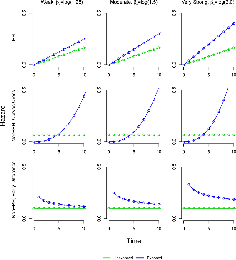
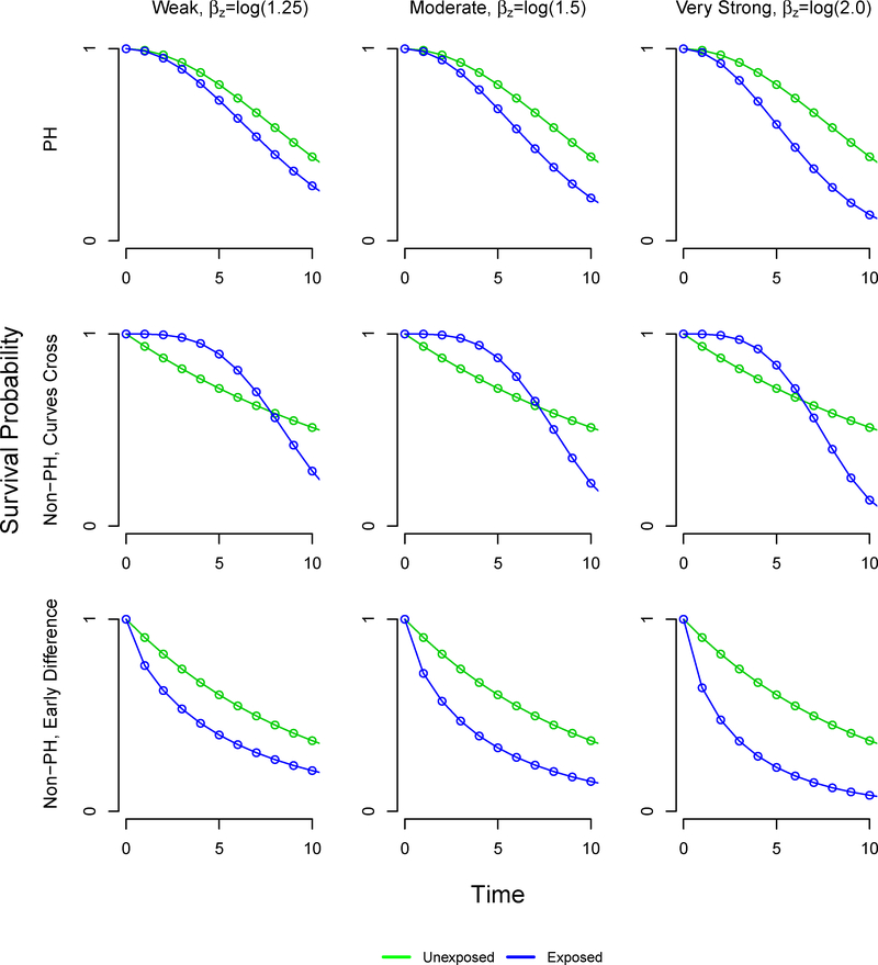
We allowed the following factors to vary: the sample size (250, 500,1000), the proportion of exposed subjects (5%, 10%, 20%, 30%, 40%, 50%), and the exposure effect exp(β_z) (1.25, 1.5, 2). In addition, we defined three settings for the time-to-event patterns: proportional hazards, non-proportional hazards with crossing survival curves, and non-proportional hazards with an early survival difference (Table 1). In the early survival difference scenarios, the HR is initially large but approaches the null value of 1 over time. The resulting survival functions are visualized in Figure A2, and the corresponding hazard functions are available in the Appendix. We thus examined 54 scenarios with 1000 simulated datasets of size n=1000, n=500, and n=250 each.

TABLE 1.

Simulation scenarios

	Unexposed		Exposed
Setting	v0	λ0	v1	λ1
Proportional hazards	2	0.0083	2	0.0100
Non-proportional hazards, survival curves cross	1	0.0667	15	0.0003
Non-proportional hazards, early survival difference	1	0.0100	10	0.2207

v and λ denote the shape and scale parameters of the Weibull distributions.

4.3. Statistical analysis in simulated datasets

We pre-specified the time point τ = 10 years for all analyses using the simulated datasets. In each simulated dataset, we estimated the difference in adjusted RMST, θ_i, between exposed and unexposed subjects. For the proposed method, we estimated the probability of being exposed using a logistic regression model of the exposure z as a function of the 7 covariates (x₁, x₂, x₃, x₄, x₅, x₆, x₇) that affect the exposure. This allowed us to obtain adjusted Kaplan-Meier estimates of the survival function in the exposed and unexposed groups, respectively. Each adjusted RMST was estimated by integration of the corresponding survival function up to τ. The standard error of the difference in adjusted RMST was estimated as described in Section 3.2.

We also used the ANCOVA-type and pseudo-observation methods as comparators. Both RMST models included the exposure variable z and all covariates associated with the time to event (x₂, x₄, x₆, x₇, x₈, x₉, x₁₀) through an identity link function. A key difference between our proposed method and the regression-based methods is that the regression-based methods can identify covariates predictive of the outcome.

4.4. Assessment of statistical performance

We assessed the statistical performance of each method of estimating the marginal effect in terms relative bias, mean squared error, empirical coverage rate, and relative error of the model-based standard errors with respect to the empirical standard errors.³⁴ To determine the marginal difference in RMST, θ, between exposed and unexposed subjects, we generated a dataset consisting of 1,000,000 subjects. We generated the covariates (x₁ to x₁₀) and exposure z as described previously. We generated times to event t₀ first assuming that all subjects were unexposed. We then simulated times to event t₁ assuming that all subjects were exposed. For the exposed and unexposed populations separately, we estimated the RMST by integrating the Kaplan-Meier estimate of the survival function up to τ and we calculated the difference in the resulting RMSTs to obtain the marginal effect θ.

We estimated the mean difference in adjusted RMST as $\widehat{\theta }=\frac{1}{1000}{\sum }_{i=1}^{100}{\widehat{\theta }}_i$. We examined four performance criteria in estimating the true marginal difference in RMST: the mean relative bias, $(\frac{\widehat{\theta }-\theta }{\theta })$; the mean squared error of the estimated effect, $\frac{1}{1000}{\sum }_{i=1}^{1000}{({\widehat{\theta }}_i-\theta )}^2$; the empirical coverage rate, estimated as the proportion of 95% confidence intervals that covered 6; and the relative error of the model-based standard errors (ModSE) $\sqrt{\frac{1}{n_{sim}}{\sum }_{i=1}^{n_{sim}}\widehat{V}({\widehat{\theta }}_i)}$ with respect to the empirical standard errors (EmpSE), $\sqrt{\frac{1}{n_{sim}-1}{\sum }_{i=1}^{n_{sim}}({\widehat{\theta }}_i-\overline{\theta })}$, defined as $\frac{ModSE-EmpSE}{EmpSE}$.³⁴

4.5. Results

In the proportional hazard setting, our proposed method using inverse probability weighting performed consistently across settings, with negligible bias. The generated marginal effects are presented in Table 2. In the proportional hazard and non-proportional hazard with early survival difference settings, the difference in restricted mean survival time increases as the marginal effect of exposure increases. However, in the non-proportional hazard setting where survival curves cross, the difference in restricted mean survival time decreases as the marginal effect of exposure increases. Figure A1 gives the hazard function and Figure A2 gives the survival curves under each setting.

TABLE 2.

Marginal differences in restricted mean survival times for each simulation scenario

	Exposure effect
Setting	Weak βz=log(1.25)	Moderate βz=log(1.5)	Very Strong βz=log(2.0)
Proportional hazards	−0.65 yrs.	−0.96 yrs.	−1.45 yrs.
Non-proportional hazards, survival curves cross	0.97 yrs.	0.74 yrs.	0.36 yrs.
Non-proportional hazards, early survival difference	−1.36 yrs.	−1.76 yrs.	−2.36 yrs.

β_z denotes the strength of the association between the exposure and outcome.

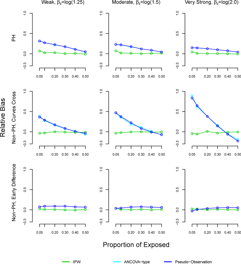
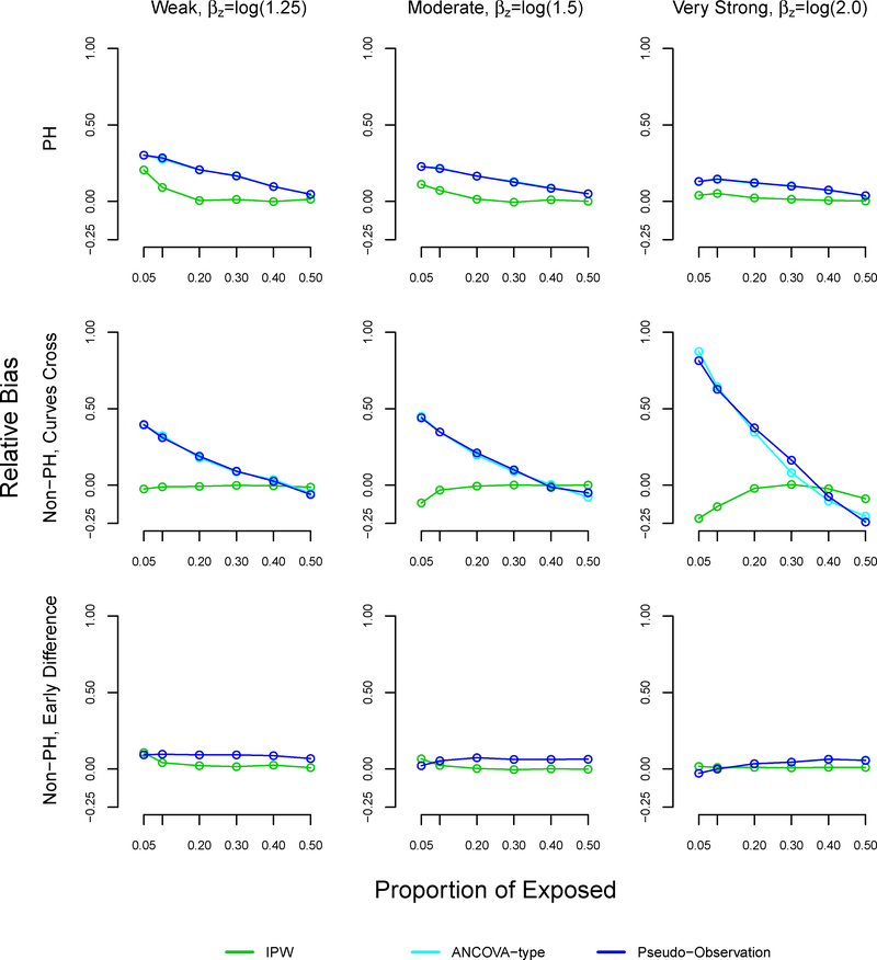
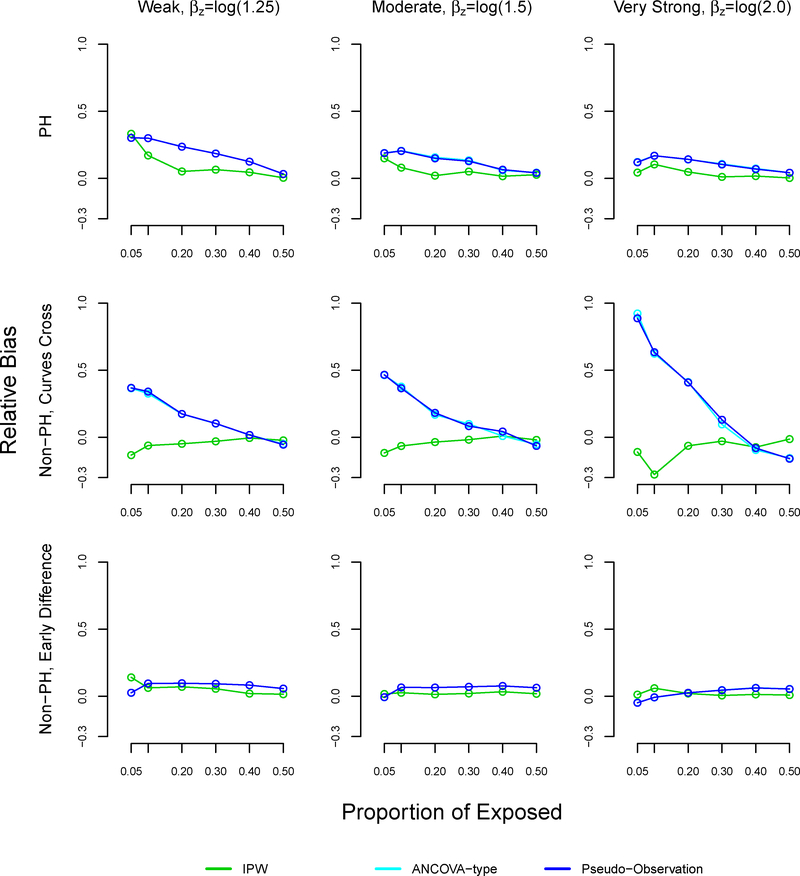
With sample size n=1000, the relative bias of the pseudo-observation and ANCOVA methods increased as the proportion of exposed decreased, reaching 32% under weak (β_z=log(1.25)) effects, 23% under moderate (β_z=log(1.5)) effects, and 15% under very strong (β_z=log(2.0)) effects at 5% exposure (Table 3, Figure A3). In the non-proportional hazard setting where survival curves cross, the trend in relative bias using the pseudo-observation and ANCOVA methods was more dramatic: the relative bias reached 38% with weak association between exposure and outcome, 46% with moderate association, and 88% with very strong association at 5% exposure. In the non-proportional hazard setting with early survival difference, all methods performed similarly in terms of relative bias.

TABLE 3.

Relative bias in simulation study, sample size n=1000

		Proportional hazards			Non-proportional hazards, curves cross			Non-proportional hazards, early survival difference
Strength of association	Proportion exposed, %	IPW	Pseudo	ANCOVA	IPW	Pseudo	ANCOVA	IPW	Pseudo	ANCOVA
Weak, βz=log(1.25)	0.05	0.070	0.317	0.317	−0.036	0.386	0.386	0.023	0.072	0.072
	0.10	0.027	0.273	0.273	−0.027	0.282	0.282	0.011	0.090	0.090
	0.20	0.026	0.219	0.219	0.001	0.182	0.182	0.008	0.091	0.091
	0.30	0.005	0.166	0.166	−0.006	0.089	0.089	−0.002	0.091	0.091
	0.40	0.009	0.116	0.116	−0.015	0.015	0.015	−0.008	0.073	0.073
	0.50	−0.009	0.040	0.040	−0.012	−0.054	−0.054	0.009	0.067	0.067
Moderate, βz=log(1.5)	0.05	0.073	0.233	0.233	−0.033	0.461	0.461	0.038	0.038	0.038
	0.10	0.020	0.217	0.217	−0.020	0.356	0.356	0.007	0.044	0.044
	0.20	0.011	0.174	0.174	−0.003	0.204	0.204	0.002	0.069	0.069
	0.30	0.002	0.124	0.124	0.002	0.096	0.096	0.010	0.075	0.075
	0.40	0.010	0.090	0.090	−0.009	0.011	0.011	−0.002	0.067	0.067
	0.50	0.015	0.046	0.046	−0.004	−0.072	−0.072	0.009	0.061	0.061
Strong, βz=log(2.0)	0.05	0.045	0.150	0.150	−0.044	0.877	0.877	0.022	−0.029	−0.029
	0.10	0.011	0.146	0.146	−0.056	0.614	0.614	0.020	0.008	0.008
	0.20	0.006	0.126	0.126	0.011	0.350	0.350	−0.001	0.036	0.036
	0.30	0.005	0.100	0.100	−0.032	0.120	0.120	0.010	0.050	0.050
	0.40	−0.001	0.076	0.076	−0.011	−0.026	−0.026	0.004	0.055	0.055
	0.50	−0.006	0.041	0.041	−0.005	−0.188	−0.188	0.000	0.053	0.053

IPW: inverse probability weighted Kaplan-Meier estimator of difference in restricted mean survival times, pseudo: pseudo-observation method of Andersen et al,^2–4 ANCOVA: ANCOVA-type method of Tian et al.¹

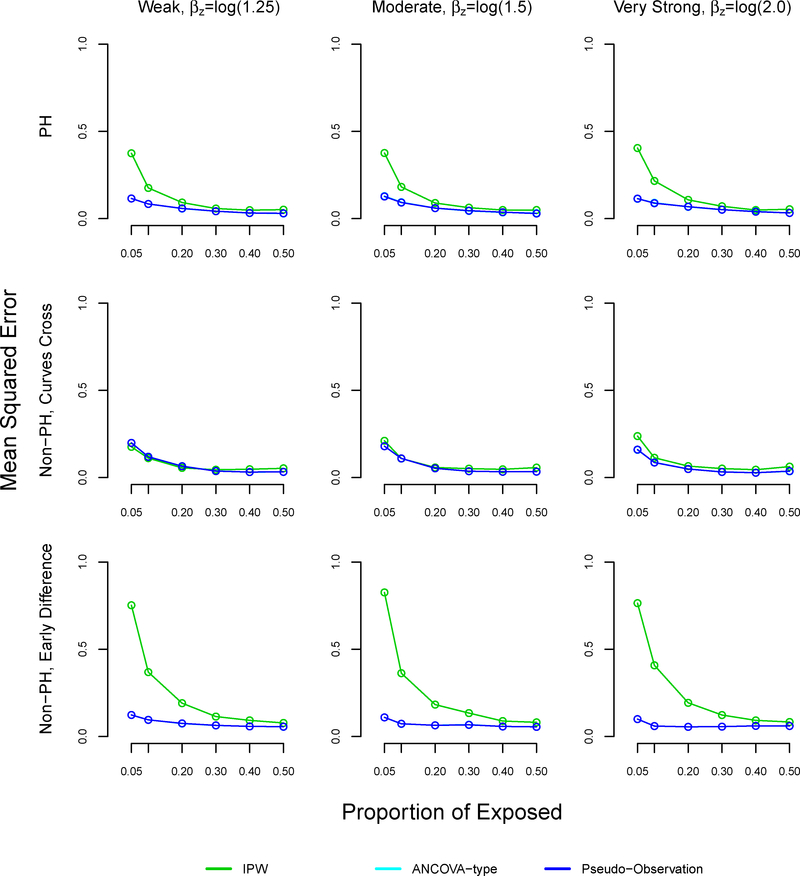
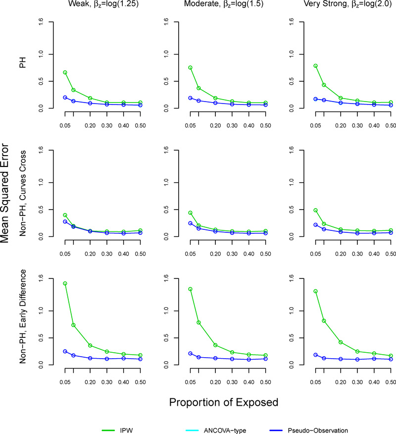
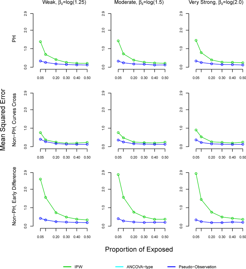
The mean squared error was similar using all methods at 50% exposure (equal size groups) (Table 4, Figure A4). However, the mean squared error increased as the proportion of exposed decreased across all settings and methods. The mean squared error was larger with the proposed method, as compared to the pseudo-observation and ANCOVA methods in the non-proportional hazards with early survival difference and proportional hazards settings, reaching 0.83 and 0.4 respectively at 5% exposure. All methods performed well in terms of MSE in the non-proportional hazards settings where survival curves cross.

TABLE 4.

Mean squared error in simulation study, sample size n=1000

		Proportional hazards			Non-proportional hazards, curves cross			Non-proportional hazards, early survival difference
Strength of association	Proportion exposed, %	IPW	Pseudo	ANCOVA	IPW	Pseudo	ANCOVA	IPW	Pseudo	ANCOVA
Weak βz=log(1.25)	0.05	0.375	0.116	0.116	0.176	0.199	0.199	0.753	0.124	0.124
	0.10	0.176	0.084	0.084	0.111	0.119	0.119	0.369	0.096	0.096
	0.20	0.092	0.058	0.058	0.056	0.065	0.065	0.191	0.075	0.075
	0.30	0.058	0.042	0.042	0.045	0.038	0.038	0.114	0.064	0.064
	0.40	0.049	0.032	0.032	0.048	0.032	0.032	0.093	0.059	0.059
	0.50	0.052	0.030	0.030	0.053	0.033	0.033	0.078	0.056	0.056
Moderate βz=log(1.5)	0.05	0.376	0.128	0.128	0.211	0.180	0.180	0.826	0.110	0.110
	0.10	0.182	0.093	0.093	0.109	0.110	0.110	0.363	0.073	0.073
	0.20	0.090	0.061	0.061	0.058	0.053	0.053	0.183	0.065	0.065
	0.30	0.063	0.044	0.044	0.051	0.036	0.036	0.134	0.068	0.068
	0.40	0.049	0.037	0.037	0.047	0.033	0.033	0.089	0.058	0.058
	0.50	0.050	0.031	0.031	0.057	0.034	0.034	0.081	0.055	0.055
Strong βz=log(2.0)	0.05	0.405	0.113	0.113	0.238	0.159	0.159	0.765	0.100	0.100
	0.10	0.216	0.090	0.090	0.114	0.087	0.087	0.408	0.060	0.060
	0.20	0.108	0.070	0.070	0.066	0.049	0.049	0.193	0.056	0.056
	0.30	0.071	0.051	0.051	0.052	0.033	0.033	0.123	0.057	0.057
	0.40	0.049	0.039	0.039	0.045	0.028	0.028	0.093	0.061	0.061
	0.50	0.054	0.031	0.031	0.063	0.036	0.036	0.083	0.060	0.060

IPW: inverse probability weighted Kaplan-Meier estimator of difference in restricted mean survival times, pseudo: pseudo-observation method of Andersen et al,^2–4 ANCOVA: ANCOVA-type method of Tian et al.¹

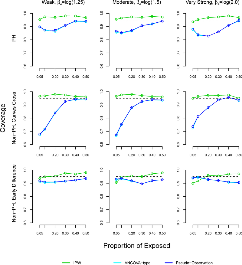
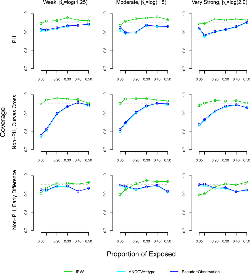
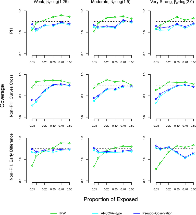
In most settings, the coverage of our method slightly surpassed 95% (Figure A5). In the non-proportional hazards settings where survival curves cross, the coverage of the pseudo-observation and ANCOVA methods decreased as the proportion of exposed decreased, reaching 67% under weak and moderate effects. These results were similar in the proportional hazards settings.

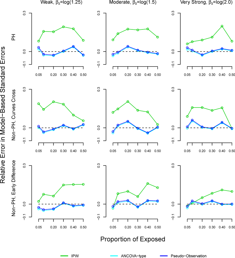
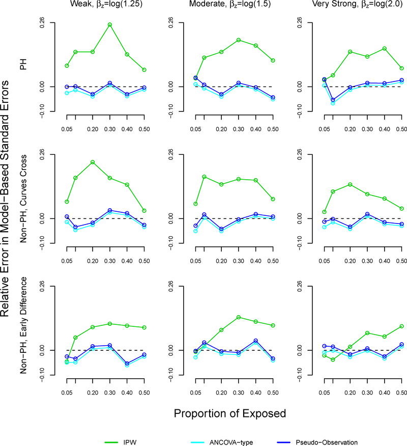
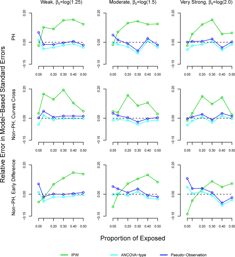
The patterns of the relative errors for our proposed method were consistent with under or over coverage, where a positive relative error indicates overcoverage and a negative relative error indicates undercoverage (Figure A6).³⁴ Morris et al suggested bias as another possible reason for under or overcoverage, however our proposed method displayed little bias.³⁴ For the pseudo-observation and ANCOVA methods, coverage appears to improve as bias decreases. However, patterns between relative errors and coverage did not hold for the pseudo-observation and ANCOVA methods. We note that our proposed method demonstrated higher relative error than the pseudo-observation and ANCOVA methods in many scenarios, sometimes reaching 20%.

Finally, results followed a similar pattern when the sample size was n=500 and n=250. The mean squared error of our proposed method increased as sample size decreased and the proportion of exposed decreased. Figures for all results are available in the appendix (Figures A3-A14).

5. Illustrative example: Framingham Heart Study

5.1. Methods

We illustrate the proposed method with the Framingham CHD 10-year risk score model. The Framingham Heart Study is a long-term prospective study of the etiology of cardiovascular disease in the community of Framingham, Massachusetts. Wilson et al examined the association between total cholesterol and 10-year risk of CHD in the Original and Offspring Cohorts.³⁷ Participants attended either the 11th examination in the Original cohort or the first examination in the Offspring cohort, and were free of CHD at baseline. Participants were followed for up to 12 years for the incidence of CHD. The exposure of interest was total cholesterol categorized as low (< 200 mg/dL), moderate (200 – 239 mg/dL), and high (≥ 240 mg/dL). The model was adjusted for age, hypertension, smoking status, diabetes, and HDL-cholesterol. Hypertension was categorized into four groups based on systolic and diastolic blood pressure, consistent with JNC-V definitions: normal including optimal (systolic <130 mmHg and diastolic <85 mmHg), high normal (systolic 130–139 mmHg or diastolic 85–89 mmHg), hypertension stage I (systolic 140–159 mmHg or diastolic 90–99 mmHg), and hypertension stages II-IV (systolic ≥ 160 mmHg or diastolic ≥ 100 mmHg).³⁸ Analyses were performed in men and women separately without formally testing for interaction. Risk factors were considered significant at a 5% two-sided level of significance. We fit the same multivariable Cox regression model for CHD, and used the same predictors to estimate the adjusted difference in RMSTs for CHD between total cholesterol groups.

We obtained adjusted HRs for high versus low total cholesterol and moderate versus low total cholesterol. We further assessed the proportional hazards assumption by the Grambsch-Thernau test at α = 0.10.³⁹ We also estimated differences in adjusted RMST between the cholesterol groups. We defined τ as 10 years for RMST measures, as Wilson et al predicted the 10-year risk of CHD. We applied our proposed method, the pseudo-observation approach, and the ANCOVA-type method to obtain the adjusted RMST. For our method, we obtained weights by fitting a multinomial logistic model to determine the individual predicted probabilities of being in each total cholesterol group according to the participant profile of all other covariates.

5.2. Results

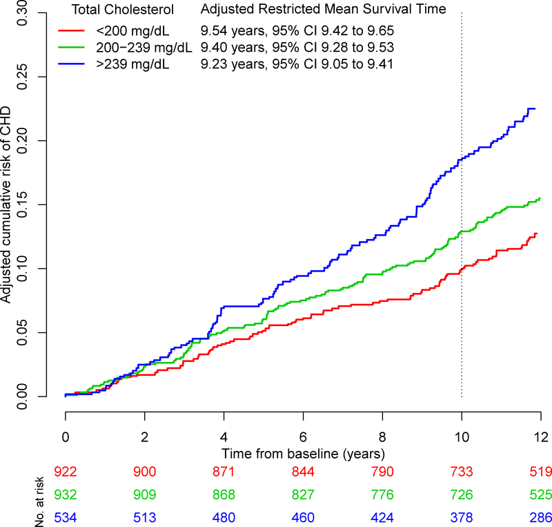
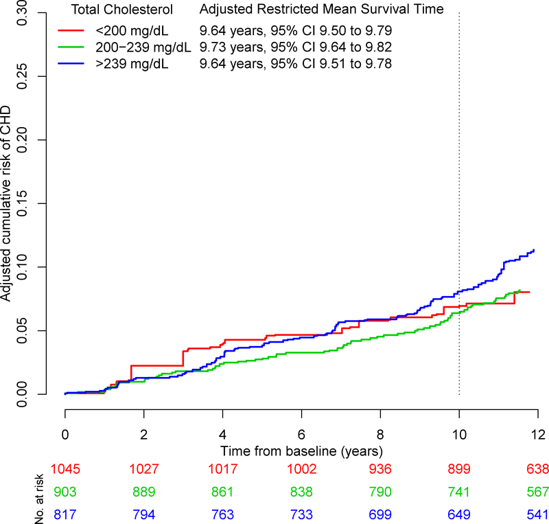
The adjusted Kaplan-Meier cumulative incidence curves and adjusted RMSTs by total cholesterol level obtained from our proposed method are presented in Figures 1 and 2, where the cumulative risk, ${\widehat{C}}_{adj}^k(t)$, is the complement of the Kaplan-Meier estimator and given by $1-{\widehat{S}}_{adj}^k(t)$. The adjusted differences in RMSTs and HRs are presented in Table 5. In both men and women, the adjusted HRs show that higher versus lower total cholesterol level is associated with CHD. The HRs of moderate versus low total cholesterol and high versus low total cholesterol were 1.3 [95% CI:1.0, 1.7] and 2.0 [95% CI:1.5, 2.6] in men and 1.7 [95% CI:1.1, 2.6] and 2.1 [95% CI:1.4, 3.2] in women.

FIGURE 1.

Adjusted Kaplan-Meier curves for coronary heart disease by total cholesterol level in men from the Framingham Heart Study

FIGURE 2.

Adjusted Kaplan-Meier curves for coronary heart disease by total cholesterol level in women from the Framingham Heart Study

TABLE 5.

Adjusted hazard ratios and differences in restricted mean survival times between total cholesterol levels in the Framingham Heart Study

	Men			Women
Method	Est.	95% CI	p	Est.	95% CI	p
Total cholesterol, 200–239 mg/dL vs. <200 mg/dL
HR	1.34	(1.03, 1.74)	0.031	1.68	(1.09, 2.57)	0.018
IPW difference in RMSTs	−1.58 mo.	(−3.58, 0.42)	0.118	1.02 mo.	(−0.98, 3.02)	0.316
Pseudo-observation difference in RMSTs	−1.57 mo.	(−3.43, 0.29)	0.097	−0.10 mo.	(−1.51, 1.32)	0.888
ANCOVA-type difference in RMSTs	−1.36 mo.	(−3.22, 0.49)	0.151	0.00 mo.	(−1.42, 1.40)	0.998
Total cholesterol, >239 mg/dL vs. <200 mg/dL
HR	1.95	(1.49, 2.56)	<.001	2.06	(1.35, 3.15)	0.001
IPW difference in RMSTs	−3.66 mo.	(−6.22,−1.10)	0.005	−0.01 mo.	(−2.36, 2.34)	0.994
Pseudo-observation difference in RMSTs	−3.46 mo.	(−5.95, −0.96)	0.006	−1.09 mo.	(−2.93, 0.74)	0.244
ANCOVA-type difference in RMSTs	−3.07 mo.	(−5.56, −0.58)	0.016	−0.95 mo.	(−2.78, 0.88)	0.309

HR: hazard ratio, IPW: inverse probability weighting, RMST: restricted mean survival time

For both moderate versus low total cholesterol and high versus low total cholesterol, the proportional hazards assumption was met among men (p=0.41 and p=0.68), but not among women (p=0.04 and p=0.04). This suggests that the adjusted HRs for women should be interpreted with caution.

With our proposed method, the adjusted mean times to CHD (RMST) for low, moderate, and high total cholesterol were 9.5, 9.4, and 9.2 years in men over a 10 year time span. In women, the adjusted mean times to CHD were 9.7, 9.7, and 9.6 years, respectively.

In men, the difference in RMSTs between moderate and low total cholesterol was similar across the three methods suggesting a small decrease in the mean time to CHD with an increase in total cholesterol: −1.6 months [95% CI: −3.6, 0.4] using our proposed method, −1.6 months [95% CI: −3.4, 0.3] with the pseudo-observation method, and −1.4 months [95% CI: −3.2, 0.5] with the ANCOVA-type method. In women, the difference in RMSTs was slightly different between methods but small to negligible: 1.0 months [95% CI: −1.0, 3.0] using our proposed method, −0.1 months [95% CI: −1.5, 1.3] with the pseudo-observation method, and 0 months [95% CI: −1.4, 1.4] with the ANCOVA-type method.

As for high versus low total cholesterol, the difference in RMSTs in men was −3.7 months [95% CI: −6.2, −1.1] using our proposed method, −3.5 months [95% CI: −6.0, −1.0] with the pseudo-observation method, and −3.1 months [95% CI: −5.6, −0.6] with the ANCOVA-type method. In women, the difference in RMSTs was −0.01 months [95% CI: −2.4, 2.3] using our proposed method, −1.1 months [95% CI: −2.9, 0.7] with the pseudo-observation method, and −1.0 months [95% CI: −2.8, 0.9] with the ANCOVA-type method.

Among both men and women, the differences in RMSTs between moderate and low total cholesterol were not significant. As for high versus low total cholesterol, the differences in RMSTs were significant among men but not in women. However, all adjusted HRs were significant. Whereas the adjusted HRs convey significant relative effects, examination of the absolute effects via difference in RMSTs gives a different picture: the mean difference in time to CHD is approximately 6 weeks in men and negligible in women, comparing moderate to low total cholesterol. The HRs and difference in RMSTs are consistent among men, but it appears that the significant HRs among women may not be clinically meaningful.

6. Discussion

We developed a method to derive adjusted RMSTs and their differences, which can be used to measure the effect of exposures or treatments in observational studies. In our simulation study, the proposed method had similar statistical performance as compared to regression-based methods previously described; all methods performed well in terms of relative bias, mean squared error, and coverage, but their advantages differed by scenario. For example, our method had lower relative bias compared to the regression-based methods in the non-proportional hazards setting where survival curves cross. However, the regression-based methods had lower mean squared error than our method in the non-proportional hazards with early survival difference setting, particularly for proportions of exposure below 30%. In our Framingham Heart Study example, all methods produced consistent RMST-based measures in men, whereas our method differed slightly from the regression-based methods in women.

Because observational studies must adjust for confounding factors, epidemiologists frequently use the Cox proportional hazards model or related approaches and typically report only adjusted hazard ratios.¹⁰ However, measures of effect based on adjusted RMST offer a different perspective. We submit that the RMST should be reported systematically alongside hazard ratios. The adjusted RMST is on the time scale, which provides clinicians and patients with background information (the adjusted RMST in the unexposed group) as well as the absolute effect of the exposure (the difference in adjusted RMST between the exposed and unexposed groups). In the Framingham Heart Study example, the adjusted HRs suggested that higher total cholesterol had a significant impact on the time to CHD, with HRs ranging from 1.3 to 2.1. In contrast, the differences in RMST between those with high versus low total cholesterol were less than 4 months in men and less than 1 month in women, over a 10 year time span. We illustrate how the difference in RMSTs can provide a different interpretation of the effect of cholesterol level on CHD risk. This is consistent with the recent work of Finegold et al, which found interventions such as statins had a mean lifespan gain of 7 months, and 95% of participants had no gain in lifespan.⁴⁰ We emphasize that the difference in RMSTs is truncated to a 10 year time span, and is not to be interpreted as a gain or loss over the lifespan. Additionally, the adjusted Kaplan-Meier curves indicate that the difference in RMSTs would continue to increase with a larger time span. If the RMSTs are reported as complementary to the HR, they would offer a tool to compare the potential of different exposures in similar target populations.⁴¹ This will assist researchers and clinicians in interpreting the impact of such exposures on outcomes.

In contrast with regression-based methods, our method is consistent with the typical RMST approach in the unadjusted framework: calculating the area below the curve. This is congruent with the visualization offered by the adjusted Kaplan-Meier curves. In randomized trials, the Kaplan-Meier graph frequently complements the reported HR due to the shortcomings of the HR’s interpretation and assumptions.¹⁰ Our approach and its implementation in R allow producing the adjusted Kaplan Meier curves. By reporting both the adjusted Kaplan-Meier curve and RMST, it is easier to gain a sense of an effect’s intensity because of the time domain. Adjusted RMST-based measures bring value to interpreting time-to-event outcomes, especially in the field of epidemiology. Additionally, randomized trials commonly report unadjusted Kaplan-Meier curves alongside unadjusted hazard ratios, yet observational studies do not report adjusted Kaplan-Meier curves. An advantage of our method is the visualization of the adjusted RMST with the adjusted Kaplan-Meier curves.

In general, Kaplan-Meier curves are not feasible with continuous covariates. Since we used adjusted Kaplan-Meier curves to calculate RMST, our method does not allow the estimation of the effect of a continuous covariate on the RMST. If the objective is to express the effect for a continuous covariate, one can use the pseudo-observation method, ANCOVA-type method, or other regression-based methods.

A limitation of adjusting Kaplan-Meier curves with inverse probability weights or propensity scores is the potential for very large or small weights.⁴² Extreme weights typically occur when there is a rare patient profile that is frequent in the adjusting population; a large weight will be assigned to this subgroup. In consequence, the survival curve will have a large variance. Therefore, the adjusted RMST also will have a large standard error. There are solutions to address extreme weights. One can stabilize weights via trimming or truncation.^30,43 Additionally, one can potentially improve the adequacy of the model by using interaction terms or exploring other model types. In our analysis, we used logistic models to estimate the propensity scores. However, there are other many options to estimate weights. For instance, models can be fit with a probit or log link rather than a logit link, or with random forest methods. However, the chosen derivation of the weights may make model-based assumptions.

A second limitation of our estimator is that we consider the weights to be fixed when deriving the variance, but in practicality, the weights may be estimated from the data. Estimating weights will introduce sampling variability, which is not accounted for in the variance. To consider the weights as random and account for the the weights being estimated from data, it is common to use adjusted sandwich variance estimators or the bootstrap.^29,44 Typically, the sandwich estimator adjusted for estimation of weights will give smaller standard errors.²⁹ Finally, Xie and Liu compared the estimated variance using estimated weights with the variance estimated from Monte Carlo simulation, and found they were comparable under various censoring scenarios.²⁷

Our simulation study compared three methods of obtaining the adjusted difference in RMST, however other methods exist which were not included in our simulation study. For example, it is possible to use piecewise exponential models, proportional hazards models, or augmented inverse-weighted Nelson-Aalen estimators.^{16–18,21–25} Although some approaches use proportional hazards models, they do not all assume proportional hazards of the exposure of interest, i.e. via stratification.^{17,18,21–25} The ANCOVA-type and pseudo-observation methods do not utilize Cox proportional hazards models. Another approach is the Royston-Parmar model that relates the log cumulative hazard function to the covariates, and in which the log baseline cumulative hazard is modeled as a cubic spline function of log time.¹² This model can be further extended for non-proportional hazards, by including an interaction term between the spline function and the covariates. Future work will entail comparing these methods as well.

Finally, we note that the Kaplan-Meier estimator is asymptotically equivalent to the Nelson-Aalen estimator. Previous works have derived the restricted mean survival time by applying inverse probability weighting to the Nelson-Aalen estimator with augmentation terms to improve efficiency. Therefore, the asymptotic results of our proposed method are a special case of previous methods using inverse-weighted Nelson-Aalen estimators if the augmentation terms are set to zero.^22–25

In conclusion, our proposed method for RMST using adjusted Kaplan-Meier curves produces results consistent with existing methods for adjusted RMST. In addition, it is congruent with the visualization of the exposure’s effect with adjusted Kaplan-Meier curves. Due to the challenging interpretation of the HR and proportional hazards assumption, we submit that the RMST should be reported systematically alongside hazard ratios. We advocate the use of RMST-based measures because of their clinically relevant interpretations. Our method offers both easily-interpreted summary measures and visualization of absolute effects through adjusted Kaplan-Meier curves, which are missing from the observational literature. It also does not rely on model assumptions, such as proportional hazards.

Appendix

A.1. Implementing the method in R

We programmed an R function, ‘akm.rmst’, based on the ‘adjusted.KM’ function in the IPWsurvival package³¹ and ‘rmstl’ function in the survRM2 package.³² This function can be used to plot adjusted survival curves and calculate the adjusted RMSTs and their difference in R. The function and a working example are available on GitHub (github.com/s-conner/akm-rmst). The ‘akm.rmst’ function requires the following arguments:

time: time to event

status: 0 if censored, 1 if event

group: factor variable for the exposure of interest

weights: user-specified weights (can be obtained through logistic models or other methods)

tau: truncation point for RMST. The default is the minimum of the each groups’ last event time.

Below, we provide a working example using the lung data from the survival package. The example is also available on GitHub.

library (survival)
data(lung)
# Drop individual with missing covariates, recode variables.
# Karnofsky performance scale index dichotomized according to clinical definitions.
lung2 <- lung [complete.cases(lung[, c (2:7, 9)]),]
lung2$male <- 2-lung2$sex
lung2$status2 <- lung2$status−1
lung2$ph.karno.low <- 0
lung2$ph.karno.low[lung2$ph.karno <=70] <- 1
# Obtain weights with logistic model, adjust for age, sex, PH.ecog, and meal.cal
logit <- glm (ph.karno.low ~ male + age + meal.cal + ph.ecog, data=lung2,
family=binomial (link= ’logit’))
pred <- predict(logit, type=’response’)
lung2$weight <- lung2$ph.karno.low/pred + (1 - lung2$ph.karno.low)/(1-pred)
# AKM RMST adjusted for age
akm_rmst(time=lung2$time, status=lung2$status2, group=as.factor (lung2$ph.karno.low),
weight=lung2$weight, tau=600)

FIGURE A1.

Weibull hazard functions defining simulation scenarios

FIGURE A2.

Weibull survival functions defining simulation scenarios

FIGURE A3.

Relative bias in simulation study for inverse probability weighting, ANCOVA-type, and pseudo-observation methods, sample size n=1000

Note: The ANCOVA and pseudo-observation approaches perform similarly, which is why the lines appear overlapping.

FIGURE A4. Mean squared error in simulation study for inverse probability weighting, ANCOVA-type, and pseudo-observation methods, sample size n=1000.

Note: The ANCOVA and pseudo-observation approaches perform similarly, which is why the lines appear overlapping.

FIGURE A5.

Coverage in 95% confidence intervals in simulation study for inverse probability weighting, ANCOVA-type, and pseudo-observation methods, sample size n=1000

Note: The ANCOVA and pseudo-observation approaches perform similarly, which is why the lines appear overlapping.

FIGURE A6.

Relative error in model-based standard errors in simulation study for inverse probability weighting, ANCOVA- type, and pseudo-observation methods, sample size n=1000

Note: The ANCOVA and pseudo-observation approaches perform similarly, which is why the lines appear overlapping. The relative error is defined as $\frac{ModSE-EmpSE}{EmpSE}$, where $ModSE=\sqrt{\frac{1}{n_{sim}}{\sum }_{i=1}^{n_{sim}}\widehat{V}({\widehat{\theta }}_i)}$ and $EmpSE=\sqrt{\frac{1}{n_{sim}-1}{\sum }_{i=1}^{n_{sim}}({\widehat{\theta }}_i-\overline{\theta })}$.

FIGURE A7.

Relative bias in simulation study for inverse probability weighting, ANCOVA-type, and pseudo-observation methods, sample size n=500

FIGURE A8. Mean squared error in simulation study for inverse probability weighting, ANCOVA-type, and pseudoobservation methods, sample size n=500.

Note: The ANCOVA and pseudo-observation approaches perform similarly, which is why the lines appear overlapping.

FIGURE A9.

Coverage in 95% confidence intervals in simulation study for inverse probability weighting, ANCOVA-type, and pseudo-observation methods, sample size n=500

FIGURE A10.

Relative error in model-based standard errors in simulation study for inverse probability weighting, ANCOVA- type, and pseudo-observation methods, sample size n=500

Note: The relative error is defined as $\frac{ModSE-EmpSE}{EmpSE}$, where $ModSE=\sqrt{\frac{1}{n_{sim}}{\sum }_{i=1}^{n_{sim}}\widehat{V}({\widehat{\theta }}_i)}$ and $EmpSE=\sqrt{\frac{1}{n_{sim}-1}{\sum }_{i=1}^{n_{sim}}({\widehat{\theta }}_i-\overline{\theta })}$.

FIGURE A11.

Relative bias in simulation study for inverse probability weighting, ANCOVA-type, and pseudo-observation methods, sample size n=250

FIGURE A12.

Mean squared error in simulation study for inverse probability weighting, ANCOVA-type, and pseudoobservation methods, sample size n=250

FIGURE A13.

Coverage in 95% confidence intervals in simulation study for inverse probability weighting, ANCOVA-type, and pseudo-observation methods, sample size n=250

FIGURE A14.

Relative error in model-based standard errors in simulation study for inverse probability weighting, ANCOVA- type, and pseudo-observation methods, sample size n=250

Note: The relative error is defined as $\frac{ModSE-EmpSE}{EmpSE}$, where $ModSE=\sqrt{\frac{1}{n_{sim}}{\sum }_{i=1}^{n_{sim}}\widehat{V}({\widehat{\theta }}_i)}$ and $EmpSE=\sqrt{\frac{1}{n_{sim}-1}{\sum }_{i=1}^{n_{sim}}({\widehat{\theta }}_i-\overline{\theta })}$.

References

- 1.Tian L, Zhao L, Wei L. Predicting the restricted mean event time with the subject’s baseline covariates in survival analysis. Biostatistics 2014; 15(2): 222–233. [DOI] [PMC free article] [PubMed] [Google Scholar]
- 2.Andersen PK, Hansen MG, Klein JP. Regression analysis of restricted mean survival time based on pseudo-observations. Lifetime Data Anal 2004; 10(4): 335–350. [DOI] [PubMed] [Google Scholar]
- 3.Andersen PK, Perme MP. Pseudo-observations in survival analysis. Stat Methods Med Res 2010; 19: 71–99. [DOI] [PubMed] [Google Scholar]
- 4.Andersen PK. Decomposition of number of life years lost according to causes of death. Stat Med 2013; 32(30): 5278–5285. [DOI] [PubMed] [Google Scholar]
- 5.Blagoev KB, Wilkerson J, Fojo T. Hazard ratios in cancer clinical trials - a primer. Nat Rev Clin Oncol 2012; 9(3): 178–183. [DOI] [PMC free article] [PubMed] [Google Scholar]
- 6.Trinquart L, Jacot J, Conner SC, Porcher R. Comparison of Treatment Effects Measured by the Hazard Ratio and by the Ratio of Restricted Mean Survival Times in Oncology Randomized Controlled Trials. J Clin Oncol 2016; 34(15): 1813–1819. [DOI] [PubMed] [Google Scholar]
- 7.Poole C On the origin of risk relativism. Epidemiology 2010; 21(1): 3–9. [DOI] [PubMed] [Google Scholar]
- 8.Poole C Commentary: some thoughts on consequential epidemiology and causal architecture. Epidemiology 2017; 28(1): 6–11. [DOI] [PubMed] [Google Scholar]
- 9.Spiegelman D, VanderWeele TJ. Evaluating Public Health Interventions: 6. Modeling Ratios or Differences? Let the Data Tell Us. Am J Public Health 2017; 107(7): 1087–1091. [DOI] [PMC free article] [PubMed] [Google Scholar]
- 10.Hernán MA. The hazards of hazard ratios. Epidemiology 2010; 21(1): 13. [DOI] [PMC free article] [PubMed] [Google Scholar]
- 11.Royston P, Parmar MK. The use of restricted mean survival time to estimate the treatment effect in randomized clinical trials when the proportional hazards assumption is in doubt. Stat Med 2011; 30(19): 2409–2421. [DOI] [PubMed] [Google Scholar]
- 12.Royston P, Parmar MK. Restricted mean survival time: an alternative to the hazard ratio for the design and analysis of randomized trials with a time-to-event outcome. BMC Med Res Methodol 2013; 13(1): 152. [DOI] [PMC free article] [PubMed] [Google Scholar]
- 13.Uno H, Claggett B, Tian L, et al. Moving beyond the hazard ratio in quantifying the between-group difference in survival analysis. J Clin Oncol 2014; 32(22): 2380–2385. [DOI] [PMC free article] [PubMed] [Google Scholar]
- 14.Zhao L, Claggett B, Tian L, et al. On the restricted mean survival time curve in survival analysis. Biometrics 2016; 72(1): 215–221. [DOI] [PMC free article] [PubMed] [Google Scholar]
- 15.Uno H, Wittes J, Fu H, et al. Alternatives to hazard ratios for comparing the efficacy or safety of therapies in noninferiority studies. Ann Intern Med 2015; 163(2): 127–134. [DOI] [PMC free article] [PubMed] [Google Scholar]
- 16.Karrison T Restricted mean life with adjustment for covariates. J Am Stat Assoc 1987; 82(400): 1169–1176. [Google Scholar]
- 17.Zucker DM. Restricted mean life with covariates: modification and extension of a useful survival analysis method. J Am Stat Assoc 1998; 93(442): 702–709. [Google Scholar]
- 18.Chen PY, Tsiatis AA. Causal inference on the difference of the restricted mean lifetime between two groups. Biometrics 2001; 57(4): 1030–1038. [DOI] [PubMed] [Google Scholar]
- 19.Royston P, Parmar MK. Flexible parametric proportional-hazards and proportional-odds models for censored survival data, with application to prognostic modelling and estimation of treatment effects. Stat Med 2002; 21(15): 2175–2197. [DOI] [PubMed] [Google Scholar]
- 20.Díaz I, Colantuoni E, Hanley D, Rosenblum M. Improved precision in the analysis of randomized trials with survival outcomes, without assuming proportional hazards. 2018: 1–30. [DOI] [PubMed]
- 21.Wei G Semiparametric methods for estimating cumulative treatment effects in the presence of non-proportional hazards and dependent censoring. PhD thesis University of Michigan, 2008. [Google Scholar]
- 22.Schaubel DE, Wei G. Double inverse-weighted estimation of cumulative treatment effects under nonproportional hazards and dependent censoring. Biometrics 2011; 67(1): 29–38. [DOI] [PMC free article] [PubMed] [Google Scholar]
- 23.Zhang M, Schaubel DE. Estimating differences in restricted mean lifetime using observational data subject to dependent censoring. Biometrics 2011; 67(3): 740–749. [DOI] [PMC free article] [PubMed] [Google Scholar]
- 24.Zhang M, Schaubel DE. Contrasting treatment-specific survival using double-robust estimators. Statistics in medicine 2012; 31(30): 4255–4268. [DOI] [PMC free article] [PubMed] [Google Scholar]
- 25.Zhang M, Schaubel DE. Double-Robust Semiparametric Estimator for Differences in Restricted Mean Lifetimes in Observational Studies. Biometrics 2012; 68(4): 999–1009. [DOI] [PMC free article] [PubMed] [Google Scholar]
- 26.Cole SR, Hernán MA. Adjusted survival curves with inverse probability weights. Comput Methods Programs Biomed 2004; 75(1): 45–49. [DOI] [PubMed] [Google Scholar]
- 27.Xie J, Liu C. Adjusted Kaplan-Meier estimator and log-rank test with inverse probability of treatment weighting for survival data. StatMed 2005; 24(20): 3089–3110. [DOI] [PubMed] [Google Scholar]
- 28.Kaplan EL, Meier P. Nonparametric estimation from incomplete observations. J Am Stat Assoc 1958; 53(282): 457–481. [Google Scholar]
- 29.Fitzmaurice GM, Laird NM, Ware JH. Applied longitudinal analysis. 998 John Wiley & Sons; 2012. [Google Scholar]
- 30.Robins JM, Hernan MA, Brumback B. Marginal Structural Models and Causal Inference in Epidemiology. Epidemiology 2000; 11(5): 550–560. [DOI] [PubMed] [Google Scholar]
- 31.Le Borgne F, Foucher Y. IPWsurvival: Propensity Score Based Adjusted Survival Curves and Corresponding Log-Rank Statistic. 2017. R package version 0.5.
- 32.Uno H, Tian L, Cronin A, Battioui C, Horiguchi M. survRM2: Comparing Restricted Mean Survival Time. 2017. Rpackage version 1.0–2.
- 33.Klein JP, Gerster M, Andersen PK, Tarima S, Perme MP. SAS and R functions to compute pseudo-values for censored data regression. Comput Methods Programs Biomed 2008; 89(3): 289–300. [DOI] [PMC free article] [PubMed] [Google Scholar]
- 34.Morris TP, White IR, Crowther MJ. Using simulation studies to evaluate statistical methods. Statistics in medicine 2019. [DOI] [PMC free article] [PubMed] [Google Scholar]
- 35.Austin PC. Balance diagnostics for comparing the distribution of baseline covariates between treatment groups in propensity-score matched samples. Stat Med 2009; 28(25): 3083–3107. [DOI] [PMC free article] [PubMed] [Google Scholar]
- 36.Bender R, Augustin T, Blettner M. Generating survival times to simulate Cox proportional hazards models. StatMed 2005; 24(11): 1713–1723. [DOI] [PubMed] [Google Scholar]
- 37.Wilson PW, D’Agostino RB, Levy D, Belanger AM, Silbershatz H, Kannel WB. Prediction of coronary heart disease using risk factor categories. Circulation 1998; 97(18): 1837–1847. [DOI] [PubMed] [Google Scholar]
- 38.The fifth report of the joint national committee on detection, evaluation, and treatment of high blood pressure (JNC V). Archives of Internal Medicine 1993; 153(2): 154–183. [PubMed] [Google Scholar]
- 39.Grambsch PM, Therneau TM. Proportional hazards tests and diagnostics based on weighted residuals. Biometrika 1994; 81(3): 515–526. [Google Scholar]
- 40.Finegold JA, Shun-Shin MJ, Cole GD, et al. Distribution of lifespan gain from primary prevention intervention. Open Heart 2016; 3(1). [DOI] [PMC free article] [PubMed] [Google Scholar]
- 41.Weir I, Marshall G, Schneider J, et al. Interpretation of time-to-event outcomes in randomized trials: an online randomized experiment. Annals of Oncology 2018; 30(1): 96–102. [DOI] [PMC free article] [PubMed] [Google Scholar]
- 42.Jackson JW, Schmid I, Stuart EA. Propensity Scores in Pharmacoepidemiology: Beyond the Horizon. Current Epidemiology Reports 2017: 1–10. [DOI] [PMC free article] [PubMed] [Google Scholar]
- 43.Austin PC. The use of propensity score methods with survival or time-to-event outcomes: reporting measures of effect similar to those used in randomized experiments. Statistics in Medicine 2014; 33(7): 1242–1258. [DOI] [PMC free article] [PubMed] [Google Scholar]
- 44.Austin PC. Variance estimation when using inverse probability of treatment weighting (IPTW) with survival analysis. Statistics in medicine 2016; 35(30): 5642–5655. [DOI] [PMC free article] [PubMed] [Google Scholar]