Abstract
While both non-destructive evaluation (NDE) and structural health monitoring (SHM) share the objective of damage detection and identification in structures, they are distinct in many respects. This paper will discuss the differences and commonalities and consider ultrasonic/guided-wave inspection as a technology at the interface of the two methodologies. It will discuss how data-based/machine learning analysis provides a powerful approach to ultrasonic NDE/SHM in terms of the available algorithms, and more generally, how different techniques can accommodate the very substantial quantities of data that are provided by modern monitoring campaigns. Several machine learning methods will be illustrated using case studies of composite structure monitoring and will consider the challenges of high-dimensional feature data available from sensing technologies like autonomous robotic ultrasonic inspection.
This article is part of the theme issue ‘Advanced electromagnetic non-destructive evaluation and smart monitoring’.
Keywords: ultrasound, structural health monitoring, non-destructive evaluation, machine learning, compressive sensing, transfer learning
1. Introduction
At first sight, the current paper may seem like rather an outlier in a special issue on Advanced Electromagnetic Non-Destructive Evaluation and Smart Monitoring; however, this is not the case. The intention here is to focus on matters of ‘smart monitoring’ with a particular emphasis on the power and efficacy of machine learning in that context. In addition, a number of points will be made regarding the distinctions between non-destructive evaluation (NDE) and structural health monitoring (SHM). Although the discussion will be in the context of ultrasonic inspection methods, the authors believe that it will be of interest and value in the exploitation of other NDE technologies.
Damage detection and identification technologies tend to be grouped according to application contexts and domains; this leads to an apparent demarcation between them which is not always useful. In the case of ultrasonic inspection, the approach crosses boundaries between NDE and SHM; it is thus useful to discuss the apparent boundaries between technologies to establish if they are useful, or actually limiting. This matter is important to discuss, because it will hopefully shed light on whether other techniques commonly accepted to be NDE, could usefully be applied to SHM problems or elsewhere.
The main aim of this paper will be to show that ultrasonic inspection has benefited from the use of machine learning or data-based analysis techniques over the last few years. In fact, this observation is true of SHM generally, where the data-based approach is arguably the dominant paradigm at this time [1]. The main intention of this paper is to inspire the more widespread possibilities of using data-based analysis, alongside physics-based techniques, in other areas of NDE than ultrasound, e.g. in electromagnetic NDE. This paper will provide illustrations spanning a range of machine learning applications to NDE, from using compressive sensing to handle the large quantities of data obtained in ultrasonic inspection, to optimizing robotic scan paths for damage detection, and finally a state-of-the-art application of transfer learning.
2. Ultrasound: structural health monitoring or non-destructive evaluation?
The main engineering disciplines associated with damage detection or identification are arguably [2]:
-
—
structural health monitoring (SHM).
-
—
non-destructive evaluation (NDE).
-
—
condition monitoring (CM).
-
—
statistical process control (SPC).
In order to examine whether these terms truly distinguish disciplines, it is useful to have an organizing principle in which to discuss damage identification problems. Such an organizing principle exists for SHM in the form of Rytter’s hierarchy [3]. The original specification cited four levels, but it is now generally accepted that a five-level scheme is appropriate [1]:
-
(i)
DETECTION: the method gives a qualitative indication that damage might be present in the structure.
-
(ii)
LOCALIZATION: the method gives information about the probable position of the damage.
-
(iii)
CLASSIFICATION: the method gives information about the type of damage.
-
(iv)
ASSESSMENT: the method gives an estimate of the extent of the damage.
-
(v)
PREDICTION: the method offers information about the safety of the structure, e.g. estimates a residual life.
This structure is a hierarchy in the sense that (in most situations) each level requires that all lower-level information is available. Few SHM practitioners would argue that Rytter’s scheme captures all the main concerns in the discipline. However, one can discuss the other damage identification technologies with respect to this scheme, with some variations.
In NDE, the emphasis is different to SHM. Most methods of NDE will involve some a priori specification of the area of inspection, examples being: eddy current methods, thermography, X-ray etc. This means that location is not usually an issue; however, there are exceptions, and ultrasonic methods are a good example. Ultrasonic inspection methods are usually classed as NDE methods, and in the case of A-scan, B-scan etc. which assume a prior location, this is appropriate. However, methods based on, for example, ultrasonic Lamb-wave scattering, also have the potential to locate damage, even over reasonable distances. Good examples of the use of Lamb-wave methods abound in the literature, and there will be no attempt here to provide a survey; however, a couple of milestones will be indicated. Guided-wave methods generally have proved very powerful in applications like pipe inspection, where the waves can propagate, and thus inspect over, large distances [4]. Lamb waves are singled out where the structure of interest is plate-like, and this has proved very powerful in the inspection of composite laminates [5]. It is arguable that the prediction level is not critical for NDE as almost all inspection methods involve taking the structure out of service for more detailed analysis or repair. In fact, almost all applications will be offline. Some element of ‘prediction’ is accommodated in the general philosophy of NDE, as code-based inspections ultimately relate the estimated damage to estimated consequence, based on structural integrity calculations.1 The important parts of the identification hierarchy for NDE are thus:
-
(i)
DETECTION: the method gives a qualitative indication that damage might be present in the structure.
-
(ii)
CLASSIFICATION: the method gives information about the type of damage.
-
(iii)
ASSESSMENT: the method gives an estimate of the extent of the damage.
Two other important distinctions between SHM and NDE were highlighted above; the first relates to the sensing technology. It is generally considered that SHM will be based on permanently-installed fixed-position sensors, while in NDE, the instruments (eddy-current probe, thermographic camera etc.) will usually be brought to the structure at the point of concern. The other distinction is that many SHM specialists consider that SHM should be conducted online, or at least with relatively high frequency, in an automated fashion, whereas NDE may be conducted sporadically or only when indicated by another inspection. The conditions which allow an NDE technology to transition to an SHM technology are that the sensing instruments become inexpensive enough to install permanently with automated triggering and data acquisition, and that it is practically possible to permanently install durable sensors and obtain effective measurements. The question of expense is also tied to the requirements in terms of sensor density; many of the physical effects exploited in NDE are very local, so that many permanently-installed units would need to be installed in order to achieve adequate area coverage. An alternate scenario where local NDE can transition to SHM is where prior knowledge can be used to pinpoint ‘hot-spots’ where local damage has higher probability, or where ‘structurally significant items’ are identified.
Ultrasonic inspection has made the transition from an NDE technique to an SHM technique partly because of the evolution of inexpensive sensors—like piezoelectric patches or wafers—and the exploitation of guided-waves, which mean that waves can propagate large distances without attenuation, e.g. Lamb waves in pipelines; this means that sensor densities are reduced [6]. Other advances in ultrasonic NDE have included the use of phased arrays [7]. A phased array is simply an ultrasonic transducer containing multiple elements which can be triggered to actuate in a prescribed sequence. Phased arrays are extremely useful for large-area inspection because the waves can be steered and focussed without moving the probe. Various designs have been proposed over the years; portable probes are available for traditional NDE, but recent designs allow bonding of sensors to the structure, essentially producing an SHM system; an example is given in [8]. Given a phased array, powerful processing techniques exist for damage imaging; one such approach is total (or full) matrix capture (FMC) [9]. In FMC, every combination of actuator/sensor elements is used; from this rich dataset, algorithms like the total focussing method allow sharp imaging of damage regions [10,11].
Another powerful imaging technique which has emerged recently is wavenumber spectroscopy, which relies on the local estimation of Lamb wave wavenumber on a fine grid [12]. The latter paper is interesting also in the sense that the ultrasound is generated using a high-power laser, but sensed using a single fixed transducer; it is thus a type of hybrid of NDE and SHM as the actuation source is an instrument which must be brought to the sample. Where reciprocity holds, the same data can be acquired by using a point actuator and sensing using a full-field method like laser vibrometry [13].
The signal processing methods used in FMC and wavenumber spectroscopy are conventional, relying on Fourier transformation etc. However, one of the major developments over the last two decades in ultrasonic NDE and SHM, has been the use of data-based approaches based on machine learning. A simplified framework for using machine learning in SHM and NDE is depicted in figure 1 [1]. Data measured from a structure are pre-processed such that damage-sensitive features are extracted (feature extraction), these become a set of inputs to the machine learning model. A relationship between inputs and outputs (e.g. predicted class labels) is inferred by the machine learner (typically on a set of training input–output pairs), which generalizes to new input data points [14]. The output predictions from new inputs can be post-processed in order to make diagnostic decisions, e.g. related to Rytter’s hierarchy. There are three main problems in machine learning: classification, regression and density estimation, with examples of all three within the SHM and NDE literature [15–22], respectively (where the reference list is not intended to be exhaustive). In classification, the challenge is inferring a map from the input data to a set of categorical labels, e.g. descriptions of discrete damage locations if performing localization [15]. Regression, by contrast, seeks to infer some functional map from some set of independent inputs to their dependent outputs, and is used in problems such as mapping flight parameters to strains on aircraft components [19,20]. Lastly, density estimation is concerned with identifying the underlying distributions of data, employed in scenarios such as tool wear monitoring, where the machinist is to be alerted when a change in tool wear has occurred [22]. These latter techniques are also suited to unsupervised learning, where only input data are known during learning, typically used in novelty detection problems where the question is whether a structure has changed from a known healthy condition [23].
Figure 1.
A simplified machine learning framework for SHM and NDE.
The remainder of this paper will be concerned with illustrating the use of machine learning and showing its potential through three case studies. The first case study demonstrates the applicability of machine learning in handling the large quantities of data obtained in an inspection campaign via compressive sensing [24]. The second study presents a Bayesian optimization and robust outlier procedure that aims to speed up robotic scanning in an autonomous manner, amending the scan path to efficiently identify damaged regions [23]. Finally, the last case study shows how very recent advances in transfer learning mean diagnostic information from one structure can be used in aiding damage identification on a separate structure—enabling robotic inspection to be performed in a more autonomous manner.
3. Compressive sensing and ultrasonic non-destructive evaluation
A characteristic of ultrasound-based NDE is that the large quantifies of high-frequency data (typically in the range of one to ten MHz) are obtained from the inspection process. These large datasets cause acquisition and data-processing challenges, problematic for both physics-based and machine learning-based analysis. Typically, due to the relatively sparse information content within a waveform, two key features are extracted from the echoes of ultrasound pulses: their attenuation and time-of-flight (TOF) difference, with the latter gaining significant attention in an NDE context.
Two main approaches exist for estimating TOF: threshold and signal phase-based methods, that use these techniques to separate the main pulse from the echoes in order to compute the difference [25], and those using physical insight in order to solve a deconvolution problem to recover the impulse response function of the material being scanned [26,27]. This latter approach—a blind deconvolution problem—is equivalent to a sparse coding step in compressive sensing (under an appropriate dictionary).
Compressive sensing (CS) aims to exploit sparsity, reconstructing a signal from much fewer samples required by the Shannon-Nyquist theorem. The approach outlined here uses machine learning, in the form of a relevance vector machine (RVM) [28]—a sparse Bayesian regression tool—in order to reconstruct a compressed signal.
(a). Compressive sensing as a sparse Bayesian regression problem
Compressive sensing involves three main stages, allowing accurate signal reconstruction from a low number of measurements. The first part (equation (3.1)), assumes the signal can be represented by a low number of coefficients and some transform—meaning it is sparse in that domain—represented by a dictionary D. A key idea in CS is that the dictionary can be formed from a variety of bases, e.g. a mixture of Fourier, wavelet and polynomial bases. The second stage of CS is where a random transform Φ (where each element is standard Gaussian or Bernoulli distributed) is applied to the signal x, preserving the pairwise distances between data points (via the Johnson–Lindenstrauss Lemma [29]), forming the compressed signal z. Recovering the original signal x from an over-complete dictionary D forms an ill-posed regression problem, in equation (3.3) (as most coefficients will be zero), solved using sparse coding or sparse regression methods, such as an RVM [24].
| 3.1 |
| 3.2 |
| 3.3 |
The compressive sensing problem in equation (3.3) can be formulated as a regression problem where the output y = Φx, i.e. the randomly transformed signal. This leads to a sparse linear regression problem, t = ΦDβ + e; t is the target vector, ΦD = X form the set of bases, β are the weights and is Gaussian-distributed noise. An RVM induces sparsity through its Bayesian model structure, particularly the choice of priors on the coefficients β (equations (3.6) and (3.7)),
| 3.4 |
| 3.5 |
| 3.6 |
| 3.7 |
where and indicate Gaussian and Gamma distributions parametrized by a mean μ, covariance Σ, a shape and b rate parameters. The integral of the Gaussian-Gamma prior structure on β leads to p(β) being Student’s t distributed; this distribution places most of its probability mass around the centre with a low number of degrees of freedom, inducing sparsity. The predictive equations from the model (using Bayes rule) leads to (where are test data points),
| 3.8 |
| 3.9 |
| 3.10 |
where A = diag(α) and the hyperparameters α and σ2 are found using an expectation maximization (EM) approach in [28].
(b). Compressive sensing on ultrasound data
A demonstration of Bayesian CS (using the RVM formulation) in estimating waveforms from C-scan data is presented in this section. A robotic head, with a water-coupled ultrasound probe consisting of 64 transducers, was used to scan a 1.2 m × 3 m composite panel. Each transducer, which can fire a 5 MHz tone burst, also acts as a receiver, where the spatial resolution of the scan was adjusted to be 0.8 mm in the direction of probe travel. Importantly, the signals all contain information at a narrow band centred around 5MHz, with the Nyquist frequency at 25 MHz, such that the problem is not oversampled (so that the trivial compression solution of decimation is not possible). An acquisition time of 24.64 μs was used to capture the range of depths in the specimen, which equates to 1232 samples at a sample rate of 50 MHz. CS results are shown in figure 2, where different dictionaries have been used; a model-based tone-burst, k-means clustering [30], and online matrix factorization. Visually, the mean reconstructed signal (indicated by the red line) is in good agreement with the measured data, with the main difference being the uncertainty in the reconstruction. In this example, a k-means dictionary [30] (an unsupervised clustering algorithm) was found to be the most appropriate, highlighting the usefulness of machine learning both in reconstruction of the signal and identifying an optimal dictionary. It can be concluded from this example, that machine learning-based CS can be used to increase both the speed and efficiency of data processing in ultrasound-based NDE.
Figure 2.
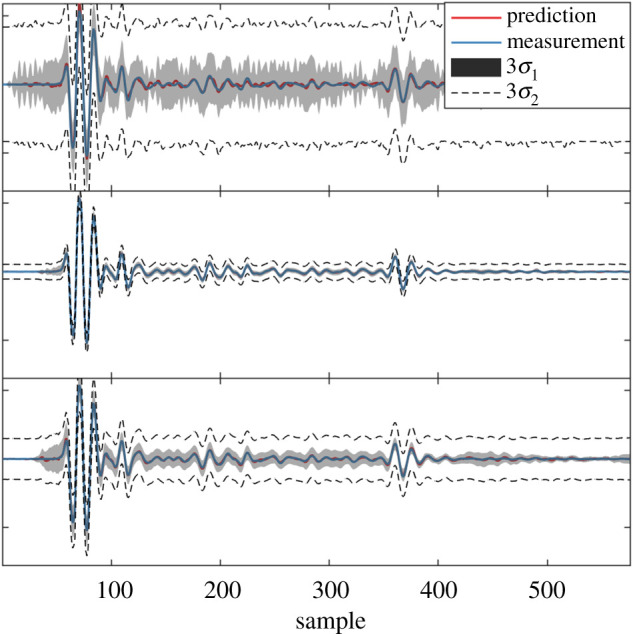
Comparison of signal reconstructions of ultrasound data using three dictionaries: (a) model-based tone-burst, (b) k-means clustering and (c) online matrix factorization. The uncertainty bounds, σ1 and σ2 refer to the prediction uncertainty without and with measurement noise, respectively [24].
4. Machine learning-based autonomous inspection
The use of robotics in NDE has changed the way NDE measurements can be acquired and has created the opportunity to automate large-scale inspection processes [31,32] (where large-scale refers to the size of the structure, e.g. a large aerospace composite panel). However, although data acquisition can be automated, it is increasingly desired that the whole inspection process, from data collection to decision about the health state of the structure, is made autonomously. This section looks at the problem of efficiently identifying damage on a specimen by performing damage detection autonomously using robust outlier analysis, and optimizing the scan path such that any damage is found efficiently using Bayesian optimization [23].
(a). Autonomous inspection strategy
The proposed inspection strategy seeks to select scanning points in a sequential manner,—rather than a uniform grid—by posing the problem as one of Bayesian optimization to maximize an objective function i.e. the ‘novelty index’ of a measured data point. The objective function is formed from a robust novelty index, as this describes the dissimilarity of a given data point against the group, while ensuring the measure is not biased by noise or the presence of damage in the group. This choice of objective function means optimization identifies spatial areas of interest that are particularly novel, and therefore likely to be damaged. The Bayesian optimization approach means that the uncertainty across the spatial field is decreased while focussing on identifying potential damage locations, with the smallest number of measurement points.
The process can be summarized as: (1) obtain data and evaluate features, (2) update robust mean and covariance estimates (including the latest data point) using fast minimum covariance determinant (FASTMCD) [33], and calculate novelty indices for the entire set,2 (3) condition the Gaussian process (GP) model [34] on the new novelty indices, (4) compute the expected improvement (EI) to find the next scan location.
EI is a utility that seeks to find a balance between exploration and exploitation [35], making it ideal for exploring the specimen while accurately identifying likely areas of damage. Given the focus of this paper, and in keeping with brevity, the interested reader is referred to [23] for more details, specifically on Gaussian Process regression, Bayesian optimization and robust outlier analysis.
A key advantage of using Bayesian optimization is that the posterior GP output is probabilistic, , leading to a probabilistic estimate of novelty scores over a two-dimensional spatial field. Typically, in outlier analysis, an observation is flagged as abnormal if its novelty index exceeds the damage threshold T. In the Bayesian optimization approach, the probability of damage (POD) is the probability that the uncertain measurement lies above the threshold p(y*,i > T) = Φ((mi − T)/vi), where Φ( · ) is a standard Gaussian cumulative density function. The method can, therefore, be used to construct a spatial POD map of the specimen, given the current scan locations.
(b). Autonomous inspection of a composite specimen
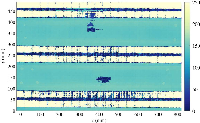
An example of the strategy is demonstrated on an industrial, carbon fibre reinforced polymer (CFRP) specimen (part of an aerospace substructure provided by Spirit Aerospace), shown in figure 3b. The specimen was known to have two main areas of delamination in the flat section of the panel, as indicated by the TOF in figure 4. Ultrasonic pulse-echo scans were acquired using a system based on a six-axis KUKA robot with a 64-element phased-array probe, as described in [32]. As the inspection strategy depends on a novelty index score, each implementation of the technique is limited to areas of ‘similar’ properties (otherwise ‘healthy’ areas with different properties would be flagged as novel given the majority ‘healthy’ area); for this reason only the flat sections are considered.
Figure 3.
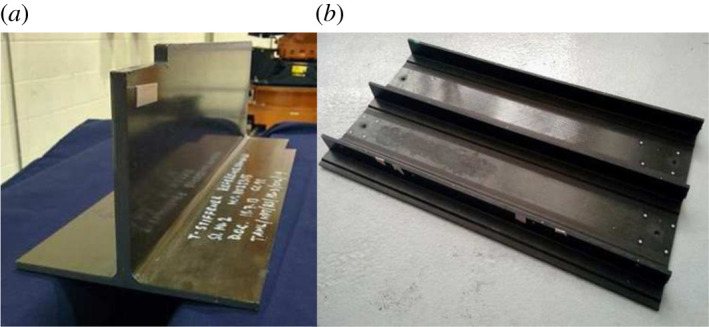
Illustration of two composite panels. (a) The source specimen used in the transfer learning case study. (b) The specimen used in the autonomous inspection case study, and is the target specimen in the transfer learning case study. (Online version in colour.)
Figure 4.
Time-of-flight map for the composite specimen (in normalized units); the target specimen in the transfer learning case study. (Online version in colour.)
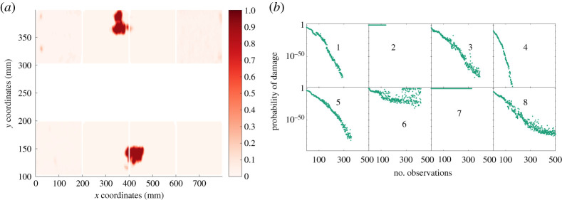
The POD, given the final observation, in each region are shown in figure 5, where it can be seen that the two main areas of damage have been identified. Furthermore, figure 5 also presents the evolution of POD for each of the eight regions, given the current observation number. It can be seen that regions 3, 6 and 7 are quickly identified as containing damage, with each requiring around 150, 400 and 300 observations, respectively. The approach therefore indicates the potential of machine learning in the automation of robotic, ultrasound-based inspection.
Figure 5.
Autonomous inspection strategy results for composite specimen [23]. (a) POD across the spatial field for the final observation in each region, (b) POD against number of observations for each discrete region (corresponding to a). (Online version in colour.)
5. Towards fully autonomous ultrasonic non-destructive evaluation: the potential of transfer learning
Another machine learning technique that could aid the transition to autonomous, ultrasound-based inspection is transfer learning. This branch of machine learning allows knowledge about damage state labels to be transferred from one structure to another, meaning datasets can be classified autonomously without the need for a human to provide labelled examples of different damage states for each new structure inspected.
As stated previously, machine learning provides multiple avenues for making decisions about the health state of a structure from data in an autonomous manner, i.e. datasets can be flagged as ‘novel’ or labelled as corresponding to a particular damage state. One challenge in using machine learning for autonomous NDE (and also in SHM) is that machine learning algorithms are typically trained, and therefore valid for, specific individual structures. This issue means that if a machine learner, trained on one specimen, was applied to another specimen, changes in the distribution of the datasets would mean that the machine learner would fail to generalize and predictions would be erroneous. In the context of ultrasound-based NDE, these changes in the data distributions between different specimens may arise for several reasons, e.g. the specimens have different nominal thicknesses; the acoustic impedance of the materials are not the same; damage types may change between specimens; manufacturing differences lead to different physical properties etc. As a result, to achieve ‘true’ autonomous robotic inspection in NDE, machine learners must overcome this limitation and generalize across a population of structures where, for many of the population, labelled data are unavailable as this requires human intervention (this is a similar goal to the related field of population-based SHM [36]).
A machine learning-based technique for transferring label knowledge between different datasets is called transfer learning. This technology seeks to leverage knowledge from a source dataset and use it in improving inferences on some target dataset. In terms of NDE, this means that for each new inspection of a new target structure, knowledge can be used from previous inspections of source structures, where labels have been collected, to aid classification of health states on the target structure, with the benefit of creating machine learners that generalize across the complete set of structures. The following case study seeks to demonstrate the potential of using transfer learning to improve damage detection on an unlabelled target composite panel based on labelled observations of a source composite panel where the features are derived from ultrasonic measurements.
(i). Domain adaptation
Domain adaptation is one branch of transfer learning [37] that seeks to map feature spaces between source data and target data , such that label knowledge can be transferred from source to target datasets; where is a matrix of feature observations from a feature space , and is a vector of labels corresponding to each feature observation in a label space . This class of methods assumes that the feature and label spaces between the source and target datasets are equal; where means the source and target features have the same dimensions Ds = Dt, and means that the same number of classes exist in the source and target spaces. Given this starting point, the key assumption in domain adaptation is that the marginal distributions of the finite feature observations for the source and target are not equal (with the potential to assume that the joint distributions are also different [38]). Consequently, the goal in domain adaptation is to find a mapping ϕ( · ) on the feature data such that (and ), meaning the source and target datasets lie on top of each other and any labelled data from the source dataset can be used to label (and therefore be transferred to) the target dataset.
(ii). Transfer component analysis
Transfer component analysis (TCA) is one method for performing domain adaptation and assumes the conditional distributions for the source and target datasets are consistent, i.e. but that the marginals are very different [39]. The technique then seeks to learn a nonlinear mapping ϕ( · ) from the feature space to a reproducing Kernel Hilbert space (RKHS), i.e via a kernel , where the distance is minimized (and therefore . The distance criterion used in TCA is the (squared) maximum mean discrepancy (MMD) distance, defined as the difference between two empirical means when the data are transformed via a nonlinear mapping into an RKHS [40],
| 5.1 |
where given that , D is the dimension of the feature space, and M is the MMD matrix,
| 5.2 |
In order to turn the distance into an optimization problem, the low-rank empirical kernel embedding [41] is exploited such that the distance can be rewritten as,
| 5.3 |
where are a set of weights to be optimized, that perform a reduction and transformation on the kernel embedding. By optimizing the weights W, the marginal distributions for the source and target features are brought together in the transformed space. Regularization in the form of a squared Frobenius-norm is applied to the optimization problem in order to control the complexity of W; in addition, the optimization is further constrained by kernel principle component analysis in order to avoid the trivial solution W = 0. The objective is formed as,
| 5.4 |
where μ controls the level of regularization, is a centring matrix, is an identify matrix and 1 a matrix of ones. The objective can be solved via Lagrangian optimization as an eigenvalue problem, where W are eigenvectors corresponding to the k-smallest eigenvalues of,
| 5.5 |
where Ψ is a diagonal matrix of Lagrange multipliers. Once the optimal W are obtained, the transformed feature space is then formed by . A classifier can now be trained in the transformed space using the labelled source data and applied to the unlabelled target data, therefore transferring the labels from source to target dataset.
(iii). Transferring non-destructive evaluation damage detection labels between composite specimens
This section presents an application of transfer component analysis in aiding robotically-enabled ultrasonic inspection of two composite aerospace panels. The task in this case study was to transfer detection labels from a source specimen with seeded defects, to data from an unlabelled target specimen that was known to have delamination damage.
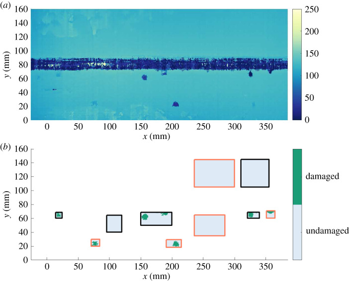
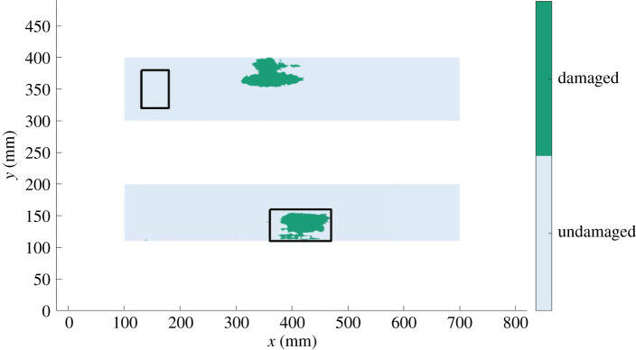
The two carbon-fibre-reinforced polymer (CFRP) specimens used in this case study are presented in figure 3 (both specimens were provided by Spirit Aerospace). Ultrasonic pulse-echo scans of both panels were acquired using a system based on a six-axis KUKA robot with a 64-element phased-array probe, described in [32]. The source specimen is representative of a typical aerospace composite, composed of a flat section with a stringer bonded to it. This panel had defects seeded into the specimen; thin sheets of poly-tetrafluoroethylene (PTFE) were inserted at different depths during manufacturing, indicated in the TOF and label maps in figure 6. The target specimen is part of an industrial aerospace structure, formed from a flat section with three stringers and stiffened areas around each stringer. Delamination was known to have occurred at two main locations on the target panel, shown in the TOF and label maps in figures 4 and 7. It is noted that the label maps in figures 6 and 7 are constructed from the known defect locations and the areas of damage are slightly larger than those indicated by the TOF maps from the raw ultrasound pulses.
Figure 6.
Source specimen. (a) Time-of-flight map (in normalized units); (b) ‘True’ label map where the black boxes indicate areas used in training both the TCA mapping and classifier, and the red boxes represent areas used in testing the classifier. (Online version in colour.)
Figure 7.
Target specimen. The ‘true’ label map where the black boxes indicate areas used in training the TCA mapping with the remaining regions being test data. (Online version in colour.)
The objective of this case study is to transfer label information from the labelled source panel, given that the seeded defects act as a proxy for delamination, and transfer this damage label to the target panel, where damage labels are assumed unknown. Furthermore, these two specimens form an interesting case study for the application of TCA, as they have different ultrasound attenuation factors caused by different ply lay-up sequences, fibre volumetric percentages etc. and both contain flat sections that have different nominal thicknesses (7 mm and 7.3 mm for the source and target, respectively) where damage is present in the flat sections of both specimens. For this reason the flat sections of each specimen are the focus of this study, as specified in the label maps in figures 6 and 7. Finally, as the goal in this case study is to transfer label knowledge from the source to target panel, only the informative parts of the source panel are used in training and testing the algorithm; which is partly due to the fact that training TCA has a computational complexity of [39]. These informative sections from the source panel are chosen as they contain representative examples of both the damaged and undamaged classes, where these sections are divided into training (black regions) and testing data (red regions) in figure 6. The black region in figure 7 relates to unlabelled target data used in inferring the TCA mapping (and are not used in training the classifier).
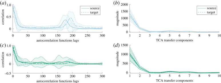
The feature spaces in this case study are normalized autocorrelation functions obtained from the raw ultrasound pulses, depicted in figure 8. In order to make the feature spaces consistent (i.e. ) the autocorrelation functions are truncated to 300 lags (i.e. D = 300) (corresponding to a time span of 12 μs), as most of the significant information in the autocorrelation functions occurs well before 300 lags. The differences in autocorrelation functions shown in figure 8 demonstrate the need for transfer learning. The distributions over the autocorrelation functions are significantly different for the source and target panels due to their geometric and material differences. It is therefore expected that a classifier trained on the source panel data will fail to correctly classify any target panel defects.
Figure 8.
(a) Mean and ±3σ (shaded region) for the source and target normalized autocorrelation functions, where undamaged and damaged classes are blue (top panel) and green (bottom panel) respectively. (b) Mean and ±3σ (shaded region) for the source and target TCA transfer components, where undamaged and damaged classes are blue (a,b) and green (c,d), respectively. (Online version in colour.)
Transfer component analysis was implemented on training data from the source and target panels (the black regions in figures 6 and 7, where the number of training data points for each panel was Ns = 7692 and Nt = 16381). The feature data were embedded using a linear kernel and TCA was implemented with a regularization factor μ = 0.1 where 10 transfer components were selected (k = 10). The inferred transfer components are presented in figure 8, where it can be seen that the transfer component distributions for the source and target panels are now ‘close’3 together and therefore a classifier trained on the source panel should generalize to the target panel.
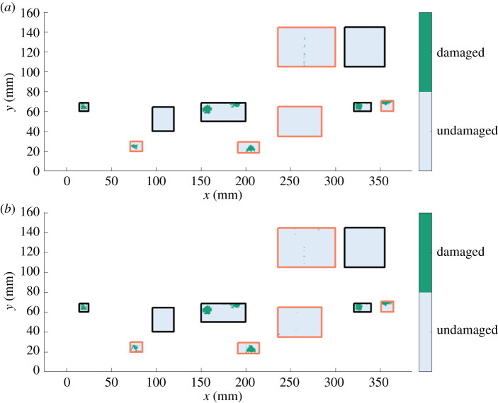
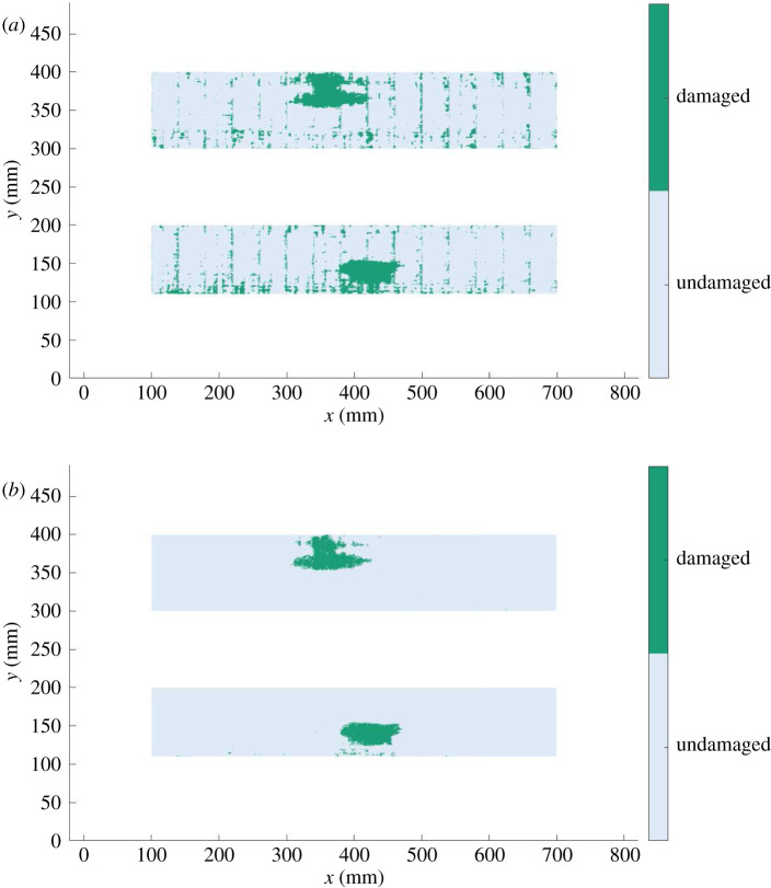
The classifier used in this case study was k-nearest neighbours (kNN), with the number of neighbours k = 1. Although any classifier could be used, kNN was selected as TCA aims to move the source and target features ‘close’ together, and therefore it would be expected that the transfer components for the source and target panels will be close in Euclidean space. Classification was performed both on the autocorrelation functions (i.e. with no transfer learning), and on the transfer components from TCA. In both scenarios, the classifier is trained on the labelled source data (black regions in figure 9) and then tested on the remaining source data (red regions in figure 9; where Ns,test = 9304) and target test data (figure 10; where Nt,test = 219910); where the features are autocorrelation functions for the no transfer learning scenario, and transfer components for TCA. The predicted labels for the source and target specimens are shown in figures 9 and 10 for the two classifiers, where visually it can be seen that there is comparable performance on the source specimen and a significant reduction in false positives for the TCA approach on the target specimen. Classification performance is quantified and compared via accuracies and macro F1-scores. These two metrics are constructed from the number of true positives (TP), false positives (FP), true negatives (TN) and false negatives (FN). Accuracy is defined as,
| 5.6 |
Figure 9.
Source specimen label predictions from the classifier trained on the source training dataset. (a) Predicted classification labels using no transfer learning; (b) predicted classification labels using TCA transfer components. The black regions are the training data and the red regions are the testing data. (Online version in colour.)
Figure 10.
Target specimen label predictions from the classifier trained on the source training dataset. (a) Predicted classification labels using no transfer learning; (b) predicted classification labels using TCA transfer components. (Online version in colour.)
The macro F1-score is formed from the precision P and recall R, for each class ,
| 5.7 |
and
| 5.8 |
where a class F1-score and macro-averaged F1-score are formed from,
| 5.9 |
and
| 5.10 |
where C is the total number of classes in . The advantage of the macro F1-score is that it equally weights the score for each class regardless of the proportion of data within each class. This property is particularly beneficial in an NDE context, as the majority of data are from the undamaged class, where poor classification of the damaged label may be masked in an accuracy score. For this reason, both accuracy and macro F1-scores are presented in table 1. The classification results clearly demonstrate the benefits in performing transfer learning in this context; visually seen from accurate label predictions in figure 10b (TCA), compared to a large number of false positives (extract green areas) in the upper panel (no transfer learning). Classification accuracy and the macro F1-score increase by 8% and 28%, respectively, when using TCA over not, with classification accuracies remaining unchanged on the source specimen using either approach. These results demonstrate that the inferred mapping is extremely beneficial in transferring label information from the source to target panel and that transfer learning is useful in progressing to a fully autonomous NDE process.
Table 1.
Classification accuracies and macro F1-scores for the transfer learning case study.
| no transfer | all data classed | |||
|---|---|---|---|---|
| method | learning | TCA | as undamaged | |
| source training | accuracy | 100.0% | 100.0% | 94.9% |
| macro F1-score | 1.000 | 1.000 | 0.487 | |
| source testing | accuracy | 98.9% | 98.9% | 97.4% |
| macro F1-score | 0.884 | 0.887 | 0.494 | |
| target testing | accuracy | 91.7% | 99.0% | 95.2% |
| macro F1-score | 0.737 | 0.943 | 0.487 |
It is interesting to note at this stage that transfer learning, particularly when using ultrasound-based features, may allow knowledge in the form of labels referring to different health states obtained from an NDE context to be used in SHM applications. This would mean that knowledge obtained in offline inspection processes could be used to make health diagnoses online, opening up the potential for more interactions between the NDE and SHM communities.
6. Discussion and conclusion
This paper opens with some discussion as to what it means for a technology to be an NDE method or an SHM method, in the context of ultrasonic inspection. The conclusion is that the boundary between methods is somewhat blurred, but largely distinguished by the sensor modality and the strategy for data acquisition. SHM is accomplished using permanently-installed sensors with data acquired continuously (or at frequent constant intervals), while NDE requires the use of external actuation/sensing and is (usually) carried out at the direction of human agency. The consideration of ultrasound as the physical basis for inspection shows that this distinction is somewhat arbitrary, with ultrasonic NDE and SHM blurring into each other. The opportunity that this realization presents, is that technology that is currently considered as restricted to offline/NDE applications, may well become a useful SHM technology if low-cost local sensing/actuation capability can be developed; at low-enough cost and high-enough durability that transducers can be permanently deployed at high enough density.
The main aim of the paper is to illustrate the power of machine learning, in carrying out data-based diagnosis in support of any physics-based prior analysis. Three case studies are presented. The first case study shows how compressive sensing (CS) can be used to store waveform data with reduced demands on computer memory or disk. CS is a lossy compression method, preserving the main features of interest; the Bayesian implementation presented in this paper has the advantage of providing confidence intervals for the reconstructed data. For transient waveforms, CS can provide a much compressed representation if an appropriate dictionary of transient basis functions is adopted. In the event that damage classifiers can be trained in the compressed domain, time and storage will be saved because the reconstruction step will not be needed. It is anticipated that CS technology will be applicable to other modes of wave-based NDE e.g. those based on acoustic emissions. The second illustration here relates to autonomous path planning for robotic inspection. A robust algorithm is presented which allows a robot system to adaptively optimize the inspection path in order to focus on probable areas of damage. Apart from the inherent intelligence of such a strategy, it offers significant reductions in scan time; furthermore, the algorithm shown here provides naturally probabilistic results.
The third and final case study discussed here is based on ongoing work, and shows how transfer learning can be used to allow inferences on structures where no damage state data are available, using data acquired from a similar but distinct structure. In the application here, NDE inspection of composite parts—representative of large aerospace structures—is carried out via an ultrasonic phased-array transducer manipulated by an industrial robotic arm. In accordance with the earlier discussion, this is clearly an NDE scenario, since the components are moved into an inspection cell, where automated analysis is executed.
It can be concluded that machine learning provides a powerful means of progress on some of the problems associated with NDE/SHM. This observation has proved true for ultrasonic methods and should be considered as an opportunity for approaches based on different physics, e.g. thermal or electrical. New methods like transfer learning overcome some of the issues of data-based methods, like the difficulty of acquiring training data that encompass all the damage states of interest.
Acknowledgements
The authors acknowledge the assistance of Spirit Aerosystems in providing the carbon composite test specimens that were scanned and analysed by the authors. The authors thank Charles Macleod who played an important role in collaborations with Spirit.
Footnotes
The authors thank one of the anonymous reviewers for this observation.
These novelty indices are inclusive outlier detection indices, and are more robust than using Mahalanobis distances, which can be affected by multiple outlying data points, masking its effects.
Where ‘close’ can be defined in terms of a distance between distributions, such as the MMD distance used in TCA.
Data accessibility
This article has no additional data.
Authors' contributions
K.W., P.G. and R.F. generated the ideas and performed the analysis in this paper. C.M. and R.F. performed the experiments and were responsible for data gathering. K.W., E.J.C. and S.G. P. were responsible for funding capture. K.W. and P.G. drafted the manuscript. E.J.C., N.D. and C.M. helped review and edit the manuscript. All authors read and approved the manuscript.
Competing interests
The authors declare that they have no conflicts of interest.
Funding
The authors acknowledge the support of the UK Engineering and Physical Sciences Research Councilvia grant nos EP/N018427/1, EP/R006768/1, EP/R003645/1, EP/S001565/1 and EP/R004900/1.
Reference
- 1.Farrar C, Worden K. 2012. Structural health monitoring: a machine learning perspective. Chichester, UK: John Wiley and Sons. [Google Scholar]
- 2.Worden K, Dulieu-Barton J. 2004. Intelligent damage identification in systems and structures. Int. J. Struct. Health Monit. 3, 85–98. ( 10.1177/1475921704041866) [DOI] [Google Scholar]
- 3.Rytter A. 1993. Vibrational based inspection of civil engineering structures. PhD. thesis, Aalborg University, Denmark.
- 4.Cawley P. 2000. Long-range inspection of structures using low frequency ultrasound. In Proc. of 2nd Int. Workshop on Damage Assessment using Advanced Signal Processing Procedures – DAMAS ’97, Sheffield, UK, pp. 1–17.
- 5.Kessler S, Spearing S, Soutis C. 2002. Damage detection in composite materials using Lamb wave methods. Smart Mater. Struct. 11, 269–278. ( 10.1088/0964-1726/11/2/310) [DOI] [Google Scholar]
- 6.Croxford A, Wilcox P, Drinkwater B, Konstantinidis G. 2007. Strategies for guided-wave structural health monitoring. Proc. R. Soc. A: Math., Phys. Eng. Sci. 463, 2961–2981. ( 10.1098/rspa.2007.0048) [DOI] [Google Scholar]
- 7.McNab A, Campbell J. 1987. Ultrasonic phased arrays for nondestructive testing. NDT Int. 20, 333–337. ( 10.1016/0308-9126(87)90290-2) [DOI] [Google Scholar]
- 8.Aranguren G, Monjel P, Cokonaj V, Barrera E, Ruiz M. 2013. Ultrasonic wave-based structural health monitoring embedded instrument. Rev. Sci. Instrum. 84, 125106 ( 10.1063/1.4834175) [DOI] [PubMed] [Google Scholar]
- 9.Li M, Hayward G. 2012. Ultrasound nondestructive evaluation (NDE) imaging with transducer arrays and adaptive processing. Sensors 12, 42–54. ( 10.3390/s120100042) [DOI] [PMC free article] [PubMed] [Google Scholar]
- 10.Chiao R, Thomas L. 1994. Analytical evaluation of sampled aperture ultrasonic imaging techniques for NDE. IEEE Trans. Ultrason., Ferroelectr. Freq. Control 41, 484–493. ( 10.1109/58.294109) [DOI] [Google Scholar]
- 11.Holmes C, Drinkwater B, Wilcox P. 2005. Post-processing of the full matrix of ultrasonic transmit-receive array data for non-destructive evaluation. NDT & E Int. 38, 701–711. ( 10.1016/j.ndteint.2005.04.002) [DOI] [Google Scholar]
- 12.Flynn E, Chong S, Jarmer G, Lee JR. 2013. Structural imaging through local wavenumber estimation of guided waves. NDT & E Int. 59, 1–10. ( 10.1016/j.ndteint.2013.04.003) [DOI] [Google Scholar]
- 13.Jeon J, Gang S, Park G, Flynn E, Kang T, Han S. 2017. Damage detection on composite structures with standing wave excitation and wavenumber analysis. Adv. Composite Mater. 26, 53–65. ( 10.1080/09243046.2017.1313577) [DOI] [Google Scholar]
- 14.Murphy K. 2012. Machine learning: a probabilistic perspective. Cambridge, MA: MIT press. [Google Scholar]
- 15.Manson G, Worden K, Allman D. 2003. Experimental validation of a structural health monitoring methodology: Part III. Damage location on an aircraft wing. J. Sound Vib. 259, 365–385. ( 10.1006/jsvi.2002.5169) [DOI] [Google Scholar]
- 16.Janssens O, Van de Walle R, Loccufier M, Van Hoecke S. 2018. Deep learning for infrared thermal image based machine health monitoring. IEEE/ASME Trans. Mechatron. 23, 151–159. ( 10.1109/TMECH.2017.2722479) [DOI] [Google Scholar]
- 17.Zhao R, Yan R, Chen Z, Mao K, Wang P, Gao RX. 2019. Deep learning and its applications to machine health monitoring. Mech. Syst. Signal Process. 115, 213–237. ( 10.1016/j.ymssp.2018.05.050) [DOI] [Google Scholar]
- 18.Bornn L, Farrar CR, Park G, Farinholt K. 2009. Structural health monitoring with autoregressive support vector machines. J. Vib. Acoust. 131, 021004 ( 10.1115/1.3025827) [DOI] [Google Scholar]
- 19.Fuentes R, Cross EJ, Halfpenny A, Worden K, Barthorpe RJ. 2014. Aircraft parametric structural load monitoring using gaussian process regression. In In the Proc. 7th European Workshop on Structural Health Monitoring.
- 20.Holmes G, Sartor P, Reed S, Southern P, Worden K, Cross E. 2016. Prediction of landing gear loads using machine learning techniques. Struct. Health Monit. 15, 568–582. ( 10.1177/1475921716651809) [DOI] [Google Scholar]
- 21.Rogers TJ, Worden K, Fuentes R, Dervilis N, Tygesen UT, Cross EJ. 2019. A Bayesian non-parametric clustering approach for semi-supervised structural health monitoring. Mech. Syst. Signal Process. 119, 100–119. ( 10.1016/j.ymssp.2018.09.013) [DOI] [Google Scholar]
- 22.Bull LA, Rogers TJ, Wickramarachchi C, Cross EJ, Worden K, Dervilis N. 2019. Probabilistic active learning: an online framework for structural health monitoring. Mech. Syst. Signal Process. 134, 106294 ( 10.1016/j.ymssp.2019.106294) [DOI] [Google Scholar]
- 23.Fuentes R, Gardner P, Mineo C, Rogers TJ, Pierce SG, Worden K, Dervilis N, Cross EJ. 2020. Autonomous ultrasonic inspection using Bayesian optimisation and robust outlier analysis. Mech. Syst. Signal Process. 145, 106897 ( 10.1016/j.ymssp.2020.106897) [DOI] [Google Scholar]
- 24.Fuentes R, Mineo C, Pierce SG, Worden K, Cross EJ. 2019. A probabilistic compressive sensing framework with applications to ultrasound signal processing. Mech. Syst. Signal Process. 117, 383–402. ( 10.1016/j.ymssp.2018.07.036) [DOI] [Google Scholar]
- 25.Kurz JH, Grosse CU, Reinhardt H. 2005. Strategies for reliable automatic onset time picking of acoustic emissions and of ultrasound signals in concrete. Ultrasonics 43, 538–546. ( 10.1016/j.ultras.2004.12.005) [DOI] [PubMed] [Google Scholar]
- 26.Legendre S, Goyette J, Massicotte D. 2001. Ultrasonic nde of composite material structures using wavelet coefficients. NDT & E Int. 34, 31–37. ( 10.1016/S0963-8695(00)00029-3) [DOI] [Google Scholar]
- 27.Cardoso G, Saniie J. 2015. Data compression and noise suppression of ultrasonic NDE signals using wavelets. In IEEE Symp. on Ultrasonics, volume 16, pp. 250–253.
- 28.Tipping ME. 2000. The relevance vector machine. In Advances in Neural Information Processing Systems, pp. 652–658. Cambridge, MA: MIT Press.
- 29.Johnson WB, Lindenstrauss J. 1984. Extensions of Lipschitz mapping into a hilbert space. Contemp. Math. 26, 189–206. ( 10.1090/conm/026/7374000) [DOI] [Google Scholar]
- 30.Bishop CM. 2006. Pattern recognition and machine learning. New York, NY: Springer. [Google Scholar]
- 31.Bogue R. 2010. The role of robotics in non-destructive testing. Ind. Robot 37, 421–426. ( 10.1108/01439911011063236) [DOI] [Google Scholar]
- 32.Mineo C, MacLeod C, Morozov M, Pierce G, Summan R, Rodden T, Kahani D, Powell J, McCubbin P, McCubbin C, Munro G, Paton S, Watson D. 2017. Flexible integration of robotics ultrasonics and metrology for the inspection of aerospace components. In AIP Conf. Proc., vol. 1806, p. 020026. [Google Scholar]
- 33.Rousseeuw P, Van Driessen K. 1999. A fast algorithm for the minimum covariance determinant estimator. Technometrics 41, 212–223. ( 10.1080/00401706.1999.10485670) [DOI] [Google Scholar]
- 34.Rasmussen C, Williams C. 2006. Gaussian processes for machine learning. Cambridge, MA: MIT Press. [Google Scholar]
- 35.Jones D, Schonlau M, Welch W. 1998. Efficient global optimization of expensive black-box functions. J. Global Optim. 13, 455–492. ( 10.1023/A:1008306431147) [DOI] [Google Scholar]
- 36.Gardner P, Liu X, Worden K. 2019. On the application of domain adaptation in structural health monitoring. Mech. Syst. Signal Process. 138, 106550 ( 10.1016/j.ymssp.2019.106550) [DOI] [Google Scholar]
- 37.Pan S, Yang Q. 2010. A survey on transfer learning. IEEE Trans. Knowl. Data Eng. 22, 1345–1359. ( 10.1109/TKDE.2009.191) [DOI] [Google Scholar]
- 38.Long M, Wang J, Ding G, Sun J, Yu P. 2013. Transfer feature learning with joint distribution adaptation. In 2013 IEEE Int. Conf. on Computer Vision, pp. 2200–2207.
- 39.Pan S, Tsang I, Kwok J, Yang Q. 2011. Domain adaptation via transfer component analysis. IEEE Trans. Neural Netw. 22, 199–210. ( 10.1109/TNN.2010.2091281) [DOI] [PubMed] [Google Scholar]
- 40.Gretton A, Borgwardt K, Rasch M, Schöolkopf B, Smola A. 2012. A kernel two-sample test. J. Mach. Learn. Res. 13, 723–773. [Google Scholar]
- 41.Schölkopf B, Smola A, Müller KR. 1998. Nonlinear component analysis as a kernel eigenvalue problem. Neural Comput. 10, 1299–1319. ( 10.1162/089976698300017467) [DOI] [Google Scholar]
Associated Data
This section collects any data citations, data availability statements, or supplementary materials included in this article.
Data Availability Statement
This article has no additional data.


