Forecasting resilience profiles of the run-up to regime shifts in nearly-one-dimensional systems

Abstract

The forecasting of sudden, irreversible shifts in natural systems is a challenge of great importance, whose realization could allow pre-emptive action to be taken to avoid or mitigate catastrophic transitions, or to help systems adapt to them. In recent years, there have been many advances in the development of such early warning signals. However, much of the current toolbox is based around the tracking of statistical trends and therefore does not aim to estimate the future time scale of transitions or resilience loss. Metric-based indicators are also difficult to implement when systems have inherent oscillations which can dominate the indicator statistics. To resolve these gaps in the toolbox, we use additional system properties to fit parsimonious models to dynamics in order to predict transitions. Here, we consider nearly-one-dimensional systems—higher dimensional systems whose dynamics can be accurately captured by one-dimensional discrete time maps. We show how the nearly one-dimensional dynamics can be used to produce model-based indicators for critical transitions which produce forecasts of the resilience and the time of transitions in the system. A particularly promising feature of this approach is that it allows us to construct early warning signals even for critical transitions of chaotic systems. We demonstrate this approach on two model systems: of phosphorous recycling in a shallow lake, and of an overcompensatory fish population.

1. Introduction

When undergoing a slow change in conditions, ecological systems can make abrupt shifts to different dynamical regimes. Regime shifts can take place in a wide variety of scenarios, regardless of whether the initial regime is an equilibrium or shows more or less regular oscillations. They are characterized by their suddenness, difficulty to anticipate and their irreversibility [1–4]. Animal populations [5] or fisheries can collapse [6], species compositions can radically alter [7], and lakes can switch from an oligotrophic to a eutrophic state [8], often with disastrous and long-enduring consequences. Much recent research has been dedicated to developing the ability to predict regime shifts [9–11] in order to allow potential negative effects to be alleviated and transitions to be reversed more quickly, or even avoided altogether. In order to do this, decision makers ideally need a reliable [12] and timely warning that a regime shift is coming [13–15], a prediction of when it is expected, and an estimate of the system resilience and any critical thresholds in the meantime [16–19]. The provision of effective early warning signals for regime shifts is a major challenge faced by researchers in ecology and many other disciplines.

At present, most of the toolbox for anticipating critical transitions is based on the tracking of early warning indicators. These are statistical measures which may show measurable trends as a system approaches a regime shift caused by disturbances or stressors, and can therefore provide warning that resilience may be declining in a system. For example, some systems close to a regime shift may exhibit critical slowing down: a slow response to perturbations [20] which can cause variance and autocorrelation to rise as a system approaches a tipping point [9,21–24], or trends in other statistical properties [25]. If multiple time series are available, these indicators can be complemented or improved by approaches based on multivariate time series analysis [26–28]. Statistical trends such as these have been observed in diverse systems in the run up to regime shifts [5,7,29,30], and there is evidence that they are robust to the time scale on which data is sampled [31]. However, because there is no absolute interpretation of such indicators they do not tell us how resilient a system is, or give actual forecasts of when the transition will come [24,32–34] unless an independent control system is also monitored for comparison [15]. Furthermore, more complicated critical transitions such as basin-boundary bifurcations of chaotic attractors and homo-/heteroclinic bifurcations of limit cycles [35–40] are poorly indicated by such methods [41,42], both because of the difficulty in separating noise-driven fluctuations from those inherent to the dynamics, and because critical slowing down can only be observed in certain regions of the state space, which are often only visited for a short time in each cycle [24,43].

In order to improve the efficacy of early warning signals, there have been calls to combine generic metric-based indicators with model-based indicators (consisting of the fitting of parsimonious models with general assumptions [32,44]), more system-specific models and details, and expert opinion [45]. But there are also properties which are shared by wide classes of systems which can be used to obtain more information about transitions in such systems without needing to completely consider system-specific detail. One such property is nearly one dimensionality [46,47]. Systems which are nearly one-dimensional (1D) can be well described by 1D maps that can be constructed from a single time series, even though they show complex dynamics and have multiple state variables. Here, we show that in such cases, we can anticipate critical transitions by fitting parsimonious models with time-dependent parameters to the nearly-1D dynamics. From these models, we can anticipate the resilience of the system in the future and the time at which regime shifts may occur. Furthermore, in this way, we can obtain model-based indicators for non-local bifurcations: when oscillatory dynamical regimes such as chaotic attractors or limit cycles collide with the basin boundary of an alternate regime and are destroyed.

The paper is structured as follows. Firstly, an overview of the method is presented, which outlines the main idea and details the techniques used. Then in the next two sections, ‘Application to a saddle-node bifurcation’ and ‘Application to a boundary crisis’, we expand on the details of the method by demonstrating its use in two particular cases: a saddle-node bifurcation in a model of phosphorous concentration in a lake, and a global bifurcation of a chaotic attractor in a discrete-time model of a harvested population. In the section ‘Data requirements’, we investigate how the effectiveness of the method depends on the quantity and timing of the available data by evaluating the performance of the method in both cases for calibration windows of different lengths and start times. Finally, in the Discussion, the approach is summarized, its assumptions are discussed and its prospects are considered.

2. Method overview

Many systems in ecology and epidemiology have been found to be nearly 1D [46–49], including various two- and three-species food web models [47,50] as well as time series taken from measles epidemics [46], Lynx fur returns and from the Nicholson blowfly experiment [47]. Even though such systems are multidimensional and continuous in time, their dynamics can be well-represented by a 1D difference equation, even in cases where they show complex dynamics such as chaos. This approximation may be obtained in two ways: firstly, from time series of a single variable using techniques derived from properties of Poincaré maps of the system (maps obtained by tracking the consecutive points where the system trajectories pass through a given plane in the space of state variables) such as the presence of next maximum or peak-to-peak maps [47,49], where each peak in the time series of a state variable is approximately given by a certain function of the previous peak; secondly from phase space reconstruction techniques such as delay embedding [51], whereby the dynamics of a system can be obtained from time-lagged observations of one or more system variables by making use of the fact that all of the system variables are linked together by the same mechanism that generates the dynamics. In its simplest case, the system dynamics can be approximated from one of its state variables by expressing the present value of this variable at time t as a function of its past value at time t − τ. The precise shape of the nearly-1D map which best approximates the dynamics, and the requirements which we need to consider, depend on the type of attractor of the system: for equilibria, we can fit a simple generic map such as a quadratic map as in [12]. For chaotic attractors, the map may need to be more complicated, but in many cases the folding of the attractor yields a simple unimodal (hump-shaped) curve in the peak-to-peak map [47]. Potentially, multiple models can be proposed and the best fitting model picked using model selection techniques such as the Akaike information criterion [52], which takes into account both the likelihood of a given model to fit the available data and how parsimonious/simple the model is, as measured by the number of model parameters.

Consider a system with slowly changing external conditions which undergoes a bifurcation-driven regime shift (also known as a B-tipping point [53]) involving an attractor colliding with the boundary of the basin of a different attractor. This is a wide class of bifurcations, including local bifurcations such as saddle-node bifurcations, but also non-local bifurcations such as basin-boundary crises of limit cycles and of chaotic attractors. Because of the continuity of the construction of the nearly-1D dynamics [54], corresponding bifurcations can also generally be seen there. If we can track changes in the approximate 1D map by fitting a generic map with linearly time-dependent parameters, then we can form a model-based resilience indicator for a regime shift because we can straightforwardly infer future system states, thresholds and tipping points from it. Although autocorrelation-based methods are often designated metric-based indicators, they can also be seen as a particular example of this class of model-based indicators: autocorrelation-at-lag-1 can be obtained by fitting a linear map in the single-delay coordinates. The main difference is that since the AR(1) map is linear, it cannot provide any information on thresholds in the system.

In this paper, we consider two kinds of systems undergoing critical transitions. Firstly, in systems at equilibrium which are close to undergoing a saddle-node bifurcation (see the example in figure 1), and whose dynamics in the presence of noise can be represented by a 1D map through delay embedding, a quadratic map can be fitted to the 1D delay coordinates as in figure 2. The equilibria can be found for such a map at each time, and used to produce a resilience profile (figure 3) in which we can see any saddle-node bifurcations taking place due to the time-dependence of the parameters. The time at which this is anticipated to happen gives an estimate of the time at which a regime shift will take place in the original system. Secondly, we consider systems exhibiting more complicated behaviour such as a chaotic attractor (see the time series in figure 4), which will be reflected in the nearly-1D dynamics. If the basin of attraction is bounded, the boundary should show up here as an unstable equilibrium, but tracking changes in the attractor is not so simple because it covers a range of values, and not a single point (figure 5). However, in a unimodal map, we can find the minimum value of an attractor easily by iterating from the maximum of the map (see electronic supplementary material, appendix b). Using this technique to produce a resilience profile of the system, we can check if this minimum value will pass the unstable equilibrium forming the threshold of the regime, at which point a regime shift takes place through a boundary crisis (figure 6).

Figure 1.

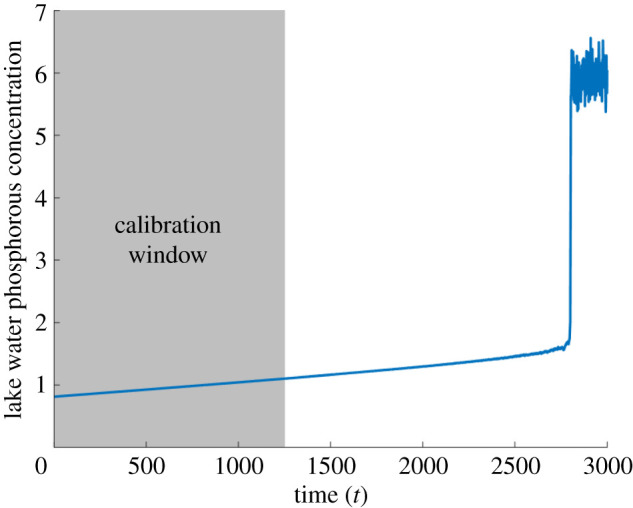
Simulated time series of the lake phosphorous concentration with linear ramping in phosphorous inflow. The system undergoes a saddle-node bifurcation at t ≈ 2800. The grey region highlights the calibration window used to fit a 1D map to the delay coordinates.

Figure 2.

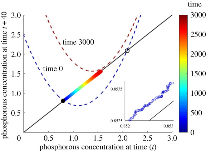
Snapshots of the fitted time-delay map from the lake phosphorous time series with delay τ = 40, taken at times t = 0 (dark blue dashed curve) and t = 3000 (dark red dashed curve). Time-series data points before the transition are shown coloured according to the corresponding time t, with a close-up of these data points shown in the inset. The stable (filled black circle) and unstable (open black circle) equilibria of the map at t = 0 are also shown.

Figure 3.

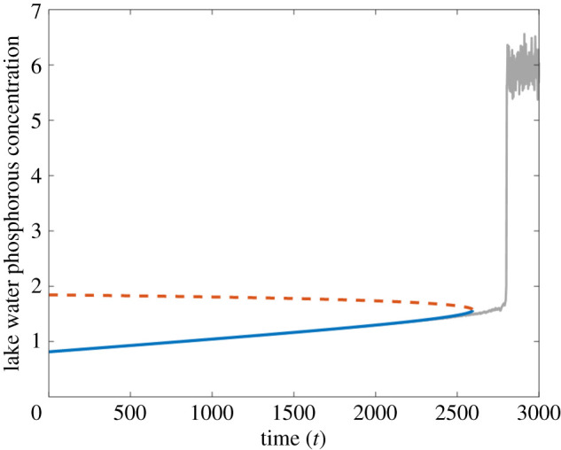
Forecast resilience profile from the lake phosphorous model. Predicted stable (blue, solid line) and unstable (orange, dashed line) equilibria, alongside the time series generated by the model (grey). The calibration window lies between t = 0 to t = 1250.

Figure 4.

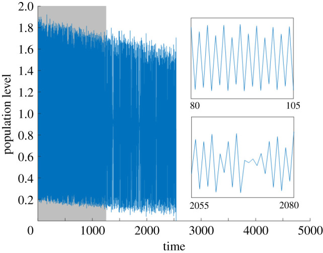
Simulated time series from the fishery model with linearly ramped harvesting (calibration window shown in grey). Subplots show stretches of the time series for which the deterministic dynamics are periodic and chaotic, respectively.

Figure 5.

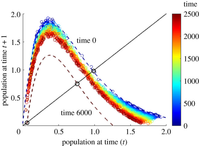
Simulated data points from the fishery model time series, coloured according to the time at which they are observed, plotted with snapshots of the time-dependent Ricker map fitted to the calibration window t ∈ [0, 1250] taken at t = 0 (dark blue dashed curve) and t = 6000 (dark red dashed curve).

Figure 6.

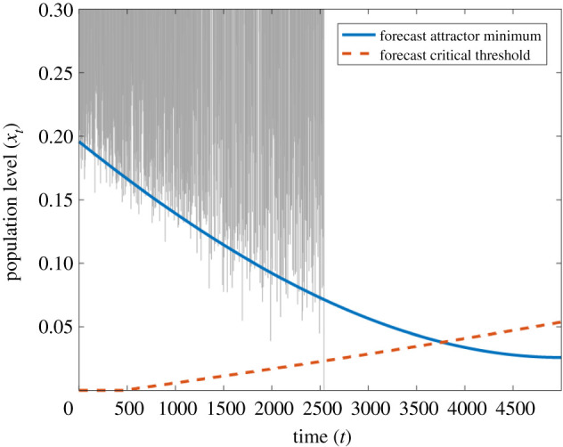
Predicted resilience profile for the harvested fish stock time series. Predicted critical threshold (orange, dashed line) and attractor minimum (blue, solid line) values, alongside the time series generated by the model (grey). The calibration window lies between t = 0 and t = 1250.

3. Application to a saddle-node bifurcation: lake water eutrophication model with ramped nutrient loading

To demonstrate how nearly-1D dynamics can be used to provide early warning signals for regime shifts, we consider a simplified model of phosphorous cycling in a lake with a slowly linearly ramped inflow of phosphorous from surrounding groundwater (see appendix A) [55].

A typical simulated time series for the phosphorous concentration in this stochastic differential equation is shown in figure 1. Initially, the system is at an equilibrium of low phosphorous concentration. As ramping of the phosphorous inflow increases, this equilibrium concentration increases with very slow acceleration, until the system suddenly jumps to a eutrophic state via a saddle-node bifurcation at t ≈ 2800. This regime shift is hard to anticipate because of its sudden nature, but it has been shown by Brock & Carpenter [55] to be accompanied by a clear increase in variance. To construct an early warning signal for this transition, we consider only the time-series data points between times 0 and 1250 as calibration ‘data’, shown by the grey region in figure 1. Although no experimental data is considered in this paper, throughout the applications sections we shall refer to simulated time series and their ‘data points’ simply as ‘time series’ and ‘data’ for the sake of brevity.

To obtain a 1D discrete-time map we can use delay embedding with a single delay variable. This entails plotting the phosphorous level at each time t with the phosphorous level at a previous time t − τ. For τ = 40, this is shown by the coloured points in figure 2 (the results are robust to variations in the choice of τ). We can then fit a simple map with linearly time-varying parameters to the delay points (x_t−τ, x_t) in the calibration window: for a non-autonomous map f(x_t, t; a), we aim to find the parameter set a which minimizes the sum of square residuals $\sum {\widehat{y_t}}^2$, where $\widehat{y_t}:=x_t-f(x_{t-\tau },t;\mathbf{a})$. In this case, a time-dependent quadratic map of the form

$$x_t=({\alpha }_0+{\alpha }_{1}t)x_{t-\tau }^2+({\beta }_0+{\beta }_{1}t)x_{t-\tau }+({\gamma }_0+{\gamma }_{1}t),$$ 3.1

is a natural, parsimonious choice to capture the saddle-node bifurcation and outperforms a linear map considerably when the Akaike Information Criterion is applied. (At first glance, this may be surprising since it seems that a straight line ought to give a better fit than the pronounced quadratics shown, because the data points lie close to the diagonal, but it makes more sense when we keep in mind the time dependence of the maps as well as the transversal response of the system to noisy perturbations that can be seen in the inset.) Extrapolation of this map beyond the times within the calibration window produces a prediction of the future system states. For the given time series and calibration window, we obtain best-fitting parameters α₀ = 1.4710, α₁ = 6.7954 × 10⁻⁵, β₀ = −3.2617, β₁ = −4.4833 × 10⁻⁴, γ₀ = 2.4913 and γ₁ = 7.4680 × 10⁻⁴. Snapshots of the fitted map at the start and end of the time series, t = 0 and t = 3000, are plotted in figure 2. In the fitted maps in figure 2, at time t = 0, we have a low-phosphorous stable equilibrium corresponding to the initial equilibrium in the original model (filled circle) and a higher unstable equilibrium (open circle) forming a threshold concentration above which eutrophication will be triggered. At t = 3000, the map is forecast to have shifted completely above the identity line, causing the two equilibria to come together and disappear in a saddle-node bifurcation, triggering a regime shift to the eutrophic state (which is not captured by the approximate discrete time map).

By tracking the equilibria of the time-dependent map along with their stability, extended beyond the calibration window, we can produce predictions for the system state, the boundary of its basin of attraction, and any bifurcations inducing a regime shift. Figure 3 shows such a forecast for the lake eutrophication model, with the original time series plotted alongside for comparison. The blue curve tracks the phosphorous concentration of the non-eutrophic state of the system. The dashed orange curve tracks the threshold concentration: if the phosphorous concentration passes above this level, a shift to the eutrophic state will be triggered. Based on the calibration data up to t = 1250, a regime shift is indicated at around 2600. This closely precedes the transition in the actual system at t ≈ 2800.

4. Application to a boundary crisis: overcompensatory population with ramped harvesting

While saddle-node bifurcations and other shifts from a regime at equilibrium are well studied, and many metric-based resilience indicators have been developed for them, non-local bifurcations such as basin-boundary crises are generally much more challenging to predict. Since nearly-1D dynamics can be obtained from time series of many systems with low-dimensional chaos in ecology and related disciplines, they offer a possible route for developing early warning signals for some of these transitions. For simplicity of presentation, we consider a 1D discrete-time system: a fishery model given by the Hassell map [56], with linearly ramped constant yield harvesting (see appendix A). Since the dynamics of this system are already 1D, a 1D map can be fitted directly to the set of consecutive points in the time series. For nearly-1D systems in general this is not possible, and peak-to-peak coordinates need to be taken (or a similar technique needs to be used) in order to fit a 1D map.

A time series obtained from this model is shown in figure 4. The Hassell map is known to display chaotic dynamics through overcompensation, and this is seen in the fish population cycles: they are irregular and show sensitivity to initial conditions. As the harvesting yield per season is ramped, the oscillations take place at lower population levels, with occasional ‘periodic windows’ in which the dynamics become more regular temporarily, until there is a collapse of the fish stock at time t ≈ 2500 due to a boundary crisis of the chaotic attractor. Essentially, as the population cycles are shifted to lower values by the increased fishing, a harvesting-driven Allee effect arises when an unstable equilibrium close to zero appears and acts as a minimum viable population level. Eventually, the minimum population level reached in the population cycles drops below this level and the fish stock collapses.

Again we consider a calibration window consisting of time points up to t = 1250, but as the data is already in discrete form, we do not need to perform delay-embedding or consider peak-to-peak maps. We can plot the x_t+1 data against the x_t data, and fit a map with parameters linearly depending on time—here we fit a Ricker map shifted in both vertical and horizontal directions

$$\begin{array}{rl}{x}_{t+1}& =[x_t-(a_0+a_{1}t)]\hspace{0.17em}\exp [(r_0+r_{1}t)(1-\frac{x_t-(a_0+a_{1}t)}{K_0+K_{1}t})]\\ & +(b_0+b_{1}t),\end{array}$$ 4.1

which is chosen as a parsimonious representation of a unimodal functional form. The best fit for such a map to this time series and calibration windows is given by the parameters r₀ = 2.580, r₁ = 2.549 × 10⁻⁶, K₀ = 0.9743, K₁ = −2.1676 × 10⁻⁶, a₀ = −0.0023, a₁ = 1.4098 × 10⁻⁶, b₀ = 0.0130 and b₁ = −9.6577 × 10⁻⁵. Snapshots of this map, together with data points from before the transition, are shown in figure 5. From the time dependence, we can extend the map beyond the calibration window and compute the critical threshold in the dynamics at each time, by finding the lowest equilibrium in the map, as well as the minimum point possibly reached in the chaotic cycles. To do this, we use the hump shape of the map which implies that the minimum of the cycles can only be reached by starting from the maximum of the map and iterating once (see electronic supplementary material, appendix b). Note that both of these extremes are computed from the maps fitted to the entire range of dynamics, instead of considering values near to the critical level alone. The difference between the minimum in the population cycles and the critical population threshold gives us the resilience of the system at each time, and tells us if a boundary crisis is possible.

By tracking the change in the population cycle minimum and the critical population threshold in time, we can obtain a resilience profile for the system as shown in figure 6. The orange dashed curve shows the critical threshold of the population level, which is predicted to increase with time, and the blue curve shows the minimum population level reached by the attractor, which is predicted to steadily decrease with time. Where these two curves cross at t ≈ 3850, we see a boundary crisis in the fitted time-dependent map. A corresponding critical transition in the original system leading to extinction of the fish population is predicted at this time. In fact, this actually happens earlier in the sample time series because noise drives the fish stock below the extinction threshold, a consequence of the resilience loss in the system. The resilience is given by the distance between the attractor minimum and the critical threshold and represents the smallest perturbation that could trigger a critical transition. However, in this case such a perturbation would need to be timed to take place when the population is at its lowest level in the chaotic cycle in order to induce a collapse.

5. Data requirements

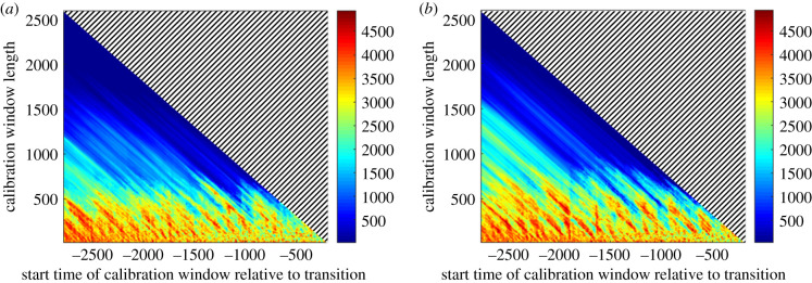
In order to gain some insight into how the characteristics of the dataset available affect the ability of nearly-1D maps to predict critical transitions, we can consider how the error in the predicted transition time changes for different windows of calibration data. A calibration window is a range of times [t₁, t₂] to which the time-dependent model is fitted, where t₁ < t₂ < t_c for a transition taking place at time t_c. Two key properties of a calibration window are its length, t₂ − t₁, and the time at which it starts, relative to the transition, t₁ − t_c. The heat maps in figure 7 show the prediction error as a function of the start time and the length of the calibration window, averaged over 10 realizations of the lake phosphorous model, for noise intensities of σ_R = 0.5% and σ_R = 1%. Here, blue regions indicate more accurate predictions, and red/orange ones indicate calibration windows giving less accurate predictions, or for which the method failed to predict a transition at all. Although we could consider that the indicator has ‘failed’ in the latter case, a considerable loss of resilience is still often predicted. Throughout the figure, a pattern of diagonal ‘streaks’ showing similarly accurate predictions is visible in spite of the averaging over multiple replicates. Since these diagonals correspond to calibration windows ending at the same time, the latest data points used for calibration have a particular significance for the accuracy of the method.

Figure 7.

Accuracy of the predictions of the transition in the lake phosphorous system as a function of the length, t₂ − t₁, and start time relative to the transition, t₁ − t_c, of the window of calibration data [t₁, t₂]. The noise intensities considered are (a) ${\sigma }_R=0.5\text{\%}$, and (b) ${\sigma }_R=1\text{\%}$. The colours represent the average absolute error in the forecast time of total resilience loss compared to that seen in the time series used for calibration. Blue regions correspond to accurate predictions and red regions to inaccurate predictions, or cases where no transition was predicted at all. Errors are averaged over 10 realizations of the model, with missed transitions being assigned an error of 5000 time points.

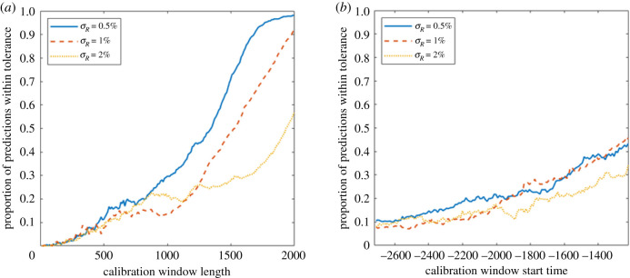
To examine how the reliability of the prediction depends on the length of available calibration data and its closeness to the transition, in figure 8 we plot the proportion of predicted transitions within 500 time points of the actual transition seen in the time series, both as a function of the length of the calibration window, t₂ − t₁, and its start time relative to the transition time, t₁ − t_c. Figure 8a shows that the length of the calibration window has a strong effect on the reliability of predictions. In order to have a greater than even chance to anticipate the saddle-node bifurcation in the lake phosphorous model, we need to have a sufficiently long calibration window available, with the required length depending on the noise intensity: around 1400 time units with ${\sigma }_R=0.5\text{\%}$, 1500 for ${\sigma }_R=1\text{\%}$ and 2000 for ${\sigma }_R=2\text{\%}$. A similar length of calibration window is necessary to reliably avoid false positives when applied to a time series without a transition (electronic supplementary material, appendix c). We also see a slight tendency for more accurate predictions the closer to the transition the time series starts (figure 8b, also visible in the shift to more prevalent blue regions in figure 7), but this is not as strong as one might expect. Note that the reason for the low proportion of acceptable predictions is that the length of the calibration window needs to be limited in order to explore a significant range of start times within the whole time series. This also holds for figure 9b.

Figure 8.

The dependence of the reliability of the predictions on the length and start time of the window of calibration data for different noise levels σ_R in the lake phosphorous system. The proportion of predicted times of total resilience loss which are within 500 time points of the actual transition time t_c (a) given a fixed length t₂ − t₁ of the calibration window and averaged over start times t₁ − t_c for t₁ ∈ [0, 600] (b) given a fixed start time t₁ − t_c and averaged over window lengths t₂ − t₁ ∈ [0, 1100]. Each set of results is averaged over 10 independent realizations of the system.

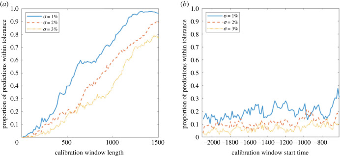
Figure 9.

The dependence of the reliability of the predictions on the length and start time of the window of calibration data for different noise levels σ in the fishery system. The proportion of predicted times of total resilience loss which are within 500 time points of the actual transition time t_c (a) given a fixed length t₂ − t₁ of the calibration window and averaged over start times t₁ − t_c for t₁ ∈ [0, 500] (b) given a fixed start time t₁ − t_c and averaged over window lengths t₂ − t₁ ∈ [0, 500]. Each set of results is averaged over 10 independent realizations of the system.

The dependence of the frequency of successful predictions on the window of calibration data for the fishery model is shown in figure 9. For this system, we take the error in the predicted transition time relative to the boundary crisis seen in the deterministic time series, rather than the stochastic time series from which the prediction is generated. This is a more fitting comparison since the fitting of time-dependent nearly-1D dynamics to the time series can only track the resilience loss caused by changes in the deterministic skeleton, while the precise time of the transition itself depends on extrinsic perturbations. Indeed, the simulated perturbations in the stochastic system essentially guarantee a considerably earlier collapse than in the deterministic case: in all the stochastic time series considered here, the crisis takes place around t = 2500 rather than ${\hat{T}}_{\det }=3718$ in the deterministic system, so that the deterministic case gives an upper bound on the time to the tipping point. Tipping points that are triggered by perturbations or noise are referred to as N-tipping points [53]. Prediction of transitions including N-tipping would involve the addition of a noise term to the time-dependent nearly-1D map, which can be done relatively straightforwardly. The data requirements for the fishery time series are similar to those of the lake phosphorous time series: the calibration window needs to be of a certain length if the method is to successfully anticipate the transition within a given accuracy, while the closeness of the calibration data to the transition has a far weaker effect.

6. Discussion

In the class of systems in which the dynamics are nearly 1D and can be well approximated by 1D discrete-time systems, there is the possibility to construct new model-based indicators for the loss of resilience and a shift to a different regime. Significantly, this can be done for challenging systems which show complicated dynamics such as chaos, as well as the more commonly studied case of systems starting at equilibrium. The approach is centred around fitting generic, parsimonious models with time-dependent parameters to the approximate 1D map in order to track how the system dynamics are changing. By doing so, we can obtain a prediction of the state of the system or its extreme values, and the thresholds beyond which the system cannot be perturbed without triggering a regime shift. This yields two important pieces of information: it tells us if and moreover when a regime shift can be expected, and it allows us to forecast the future resilience of the system, in the sense of the maximum disturbance that can be tolerated without triggering a shift. Such forecasts can either be made continuously using a moving calibration window as with metric-based early warning signals, or incorporated into an iterative forecasting framework [57].

Most existing early warning signals take metric-based approaches, in that they use trends in statistical properties of the times series, such as an increase in variance due to critical slowing down of the response to perturbations, as indicators that the system may be losing resilience or approaching a regime shift. Such indicators have many benefits in that they are generic and require no knowledge of the system monitored, at least in principle. However, these statistical trends generally do not yield quantitative estimates of the resilience of the system or forecasts of the time at which a system should undergo a transition [24,33]. One way to rectify this is to develop model-based approaches such as the one presented here to supplement metric-based indicators [32]. Model-based techniques could be applied to systems which are flagged by metric-based indicators as possibly losing resilience or approaching a critical transition, both in order to corroborate the early warning signal from the indicator and to provide extra information about the resilience loss and predict how it is likely to unfold. Although model-based methods involve the fitting of models rather than the monitoring of statistical trends, the two groups of indicators share many common assumptions. In particular, both assume a basic separation of timescales between fast state variables and slowly changing environmental conditions or parameters, as well as a distinction between intrinsic deterministic dynamics and external stochastic perturbations.

In order for the model-based approach presented here to anticipate transitions successfully, the system and the available data must satisfy additional requirements beyond the presence of nearly-1D dynamics. The assumption of a clear time-scale separation between slowly changing parameters and faster dynamical variables implies that the approach will fail in the presence of rapidly changing conditions [53]. Similarly, a particular dependence of parameters on time is required–here a linear dependence on time is assumed. Stressors in real-world systems are unlikely to increase at a precisely linear rate, but linear ramping may serve as a valid first-order approximation so long as the ramping is broadly unidirectional. When ramping in system drivers is nonlinear, predictions beyond a certain time scale will likely be inaccurate, with this time scale becoming shorter with more nonlinear ramping. Additionally, noise with too large a variance can overwhelm the time-dependence of the dynamics and cause the ‘signal’ of the gradual change in the structure of the system to become indiscernible [33]. On the other hand, in the case of systems at equilibrium such as the lake phosphorous model, sufficient noise is needed to reveal the system structure and its changes: negligible noise levels are insufficient for the system response to reveal the nearly-1D dynamics away from the equilibrium. Furthermore, a sufficiently long dataset is needed to adequately fit the time-dependent nearly-1D map, as the plots in figures 8 and 9 show. This remains a particular challenge to forecasting critical transitions in ecology, where data availability is limited.

Unlike the system properties used by many metric-based indicators, nearly-1D dynamics are not universal. There is, however, evidence that they are widespread in ecology [47,49], epidemiology [46], physiology [58,59], electronics [60] and chemical systems [61,62]. Nearly-1D dynamics are often not immediately recognizable in time series without using delay-embedding or considering peak-to-peak maps, but there are certain types of system in which they are more common. In particular, dynamics which follow low-dimensional chaotic or quasi-periodic cycles are frequently nearly-1D. Deterministic periodic systems exhibit nearly-1D dynamics which consist of jumps between a finite number of points, making the interpolation and tracking of a 1D map difficult. However, sufficient noise can change this by displacing the state from the periodic orbit and revealing more of the nearly-1D dynamics in a surrounding invariant region, even to the point of inducing stochastic chaos [63–65]. In deterministic systems at equilibrium, nearly-1D dynamics will always be given by a single point and it remains an open question for which systems noise can reveal a full nearly-1D map in this case. Some multidimensional systems show fast–slow dynamics which imply nearly-1D dynamics, but arguably they should also be seen in many more systems near tipping points: the centre manifold theorem guarantees that critical slowing down only takes place in the direction of the centre manifold [66] which will be a 1D curve for saddle-node and other types of bifurcation. Observed data points should be primarily distributed along this curve, because perturbations perpendicular to it will return more quickly than those tangent to it [67]. Time-series analysis techniques such as delay embedding may reflect this by returning nearly-1D dynamics, although the success of such techniques with substantial noise is not guaranteed [68]. Overall, however, there remains the need for similar methods for higher dimensional systems without nearly-1D dynamics. The framework presented here may be extended to such systems by, e.g. approximating their dynamics from time series using current methods such as those found in [69,70].

The additional information which we can gain by considering the nearly-1D dynamics of a system means that they can play an important role in bringing existing early warning signals closer to management decisions with the view of taking action to manage a transition or prevent it completely. Firstly, time scale is an important factor in most management strategies, because they rely on the gradual effect of physical or biological processes, the development of new technology, or simply need time to be organized [8,13]. In ecology, life-history effects and delay mean that biological interventions may only be effective on the time scale of one or more lifespans of the organisms involved [71]. The time requirements and monetary cost of management actions can necessitate estimates of the time left available in order to decide which transitions can be reversed, and which management strategies will be effective. Estimates of the resilience and critical thresholds in the run up are also useful to inform a decision as to which management measures are necessary or cost-effective—for instance, whether to take short-term measures such as keeping the state away from the threshold or longer-term measures such as moving the threshold itself [4], or whether it is even worth trying to mitigate the regime shift rather than allowing it to take place and concentrate on helping the system adapt [72,73].

Another prospect for the use of nearly-1D dynamics to guide early warning signals lies in their ability to anticipate regime shifts caused by non-local bifurcations, before which the system is not at equilibrium, but instead undergoes periodic or chaotic cycles. Such regime shifts are particularly challenging to anticipate, and many of the standard approaches in the early warning signals toolbox cannot be applied effectively at all. While these bifurcations do exhibit critical slowing down in a sense [43], statistical trends are usually lost among the intrinsic fluctuations already present, especially if they are chaotic or if the system is only close to a threshold for a small part of each cycle. The use of nearly-1D dynamics finally opens up the prospect of constructing early warning signals for these types of regime shift in certain cases.

Appendix A. Models used to produce simulated data

A.1. Lake phosphorous model

The dynamics of phosphorous in lake water are described by the following equation from [55]:

$$\frac{\text{d}x}{\text{d}t}=c_{1}U(t)-c_{2}x+c_{3}mF(x)+{\sigma }_{R}mF(x)\frac{\text{d}W}{\text{d}t}$$

and

$$F(x)=\frac{x^q}{c_4^q+x^q}.$$

x is the concentration of phosphorous in the water in g m⁻². c₁ = 0.00115 is the phosphorous inflow from groundwater, c₂ = 0.85 the outflow coefficient, c₃ = 0.019 the recycling rate, c₄ = 2.4 the recycling half-saturation coefficient, m = 200 g m⁻² the concentration of phosphorous in the lake sediment, q = 8 the recycling function exponent, and σ_R the standard deviation of stochastic perturbations to recycling (${\sigma }_R=0.5\text{\%}$ unless specified otherwise). The mass of phosphorous in the watershed soil is given by the linear function U(t) = U₀ + U₁t, where U₀ = 600 g m⁻² and U₁ = 1/6 g m⁻²〈t〉⁻¹. W is a standardized Wiener process.

A.2. Fishery model

The model for a harvested fish population with overcompensatory dynamics is given by the following equation, based on the Hassell model [56] with constant yield harvesting and multiplicative environmental noise

$$x_{t+1}=(1+\sigma \xi )[\frac{r{x}_t}{{(1+a{x}_t)}^{\beta }}-h(t)],$$

r = 13.5 is the basic growth rate, a = 0.03 the rate of density-dependent saturation, β = 90 the compensation parameter, σ is the standard deviation of the noise ($\sigma =2\text{\%}$ unless specified otherwise) and ξ is a normally distributed random variable with mean of 0 and variance of 1. Note that in the limit β = 1/a → ∞, this model convergences to the Ricker map. The harvesting yield is given by h(t) = h₀ + h₁t, where h₀ = 0, and h₁ = 1 × 10⁻⁴.

Data accessibility

The codes used to generate the results presented here can be found under https://doi.org/10.5281/zenodo.3994459.

Authors' contributions

M.W.A. contributed to the design of the study, performed the analysis and wrote the manuscript; J.H.P.D. contributed to the conception of the study and critically revised the manuscript; A.H. provided guidance on study design and analysis and critically revised the manuscript; F.H. conceived of the study, contributed to its design, and helped to draft and critically revise the manuscript.

Competing interests

We declare we have no competing interests.

Funding

No funding has been received for this article.

References

- 1.Holling CS. 1973. Resilience and stability of ecological systems. Annu. Rev. Ecol. Syst. 4, 1–23. ( 10.1146/annurev.es.04.110173.000245) [DOI] [Google Scholar]
- 2.Sutherland JP. 1974. Multiple stable points in natural communities. Am. Nat. 108, 859–873. ( 10.1086/282961) [DOI] [Google Scholar]
- 3.May RM. 1977. Thresholds and breakpoints in ecosystems with a multiplicity of stable states. Nature 269, 471–477. ( 10.1038/269471a0) [DOI] [Google Scholar]
- 4.Folke C, Carpenter S, Walker B, Scheffer M, Elmqvist T, Gunderson L, Holling C. 2004. Regime shifts, resilience, and biodiversity in ecosystem management. Annu. Rev. Ecol. Evol. Syst. 35, 557–581. ( 10.1146/annurev.ecolsys.35.021103.105711) [DOI] [Google Scholar]
- 5.Dai L, Vorselen D, Korolev KS, Gore J. 2012. Generic indicators for loss of resilience before a tipping point leading to population collapse. Science 336, 1175–1177. ( 10.1126/science.1219805) [DOI] [PubMed] [Google Scholar]
- 6.Mullon C, Fréon P, Cury P. 2005. The dynamics of collapse in world fisheries. Fish Fish. 6, 111–120. ( 10.1111/j.1467-2979.2005.00181.x) [DOI] [Google Scholar]
- 7.Carpenter SR. et al. 2011. Early warnings of regime shifts: a whole-ecosystem experiment. Science 332, 1079–1082. ( 10.1126/science.1203672) [DOI] [PubMed] [Google Scholar]
- 8.Carpenter SR, Ludwig D, Brock WA. 1999. Management of eutrophication for lakes subject to potentially irreversible change. Ecol. Appl. 9, 751–771. ( 10.1890/1051-0761(1999)009[0751:MOEFLS]2.0.CO;2) [DOI] [Google Scholar]
- 9.Carpenter SR, Brock WA. 2006. Rising variance: a leading indicator of ecological transition. Ecol. Lett. 9, 311–318. ( 10.1111/j.1461-0248.2005.00877.x) [DOI] [PubMed] [Google Scholar]
- 10.Scheffer M. 2009. Critical transitions in nature and society. Princeton, NJ: Princeton University Press. [Google Scholar]
- 11.Scheffer M. et al. 2012. Anticipating critical transitions. Science 338, 344–348. ( 10.1126/science.1225244) [DOI] [PubMed] [Google Scholar]
- 12.Boettiger C, Hastings A. 2012. Quantifying limits to detection of early warning for critical transitions. J. R. Soc. Interface 9, 2527–2539. ( 10.1098/rsif.2012.0125) [DOI] [PMC free article] [PubMed] [Google Scholar]
- 13.Biggs R, Carpenter SR, Brock WA. 2009. Turning back from the brink: Detecting an impending regime shift in time to avert it. Proc. Natl Acad. Sci. USA 106, 826–831. ( 10.1073/pnas.0811729106) [DOI] [PMC free article] [PubMed] [Google Scholar]
- 14.Contamin R, Ellison AM. 2009. Indicators of regime shifts in ecological systems: What do we need to know and when do we need to know it. Ecol. Appl. 19, 799–816. ( 10.1890/08-0109.1) [DOI] [PubMed] [Google Scholar]
- 15.Pace ML, Batt RD, Buelo CD, Carpenter SR, Cole JJ, Kurtzweil JT, Wilkinson GM. 2017. Reversal of a cyanobacterial bloom in response to early warnings. Proc. Natl Acad. Sci. USA 114, 352–357. ( 10.1073/pnas.1612424114) [DOI] [PMC free article] [PubMed] [Google Scholar]
- 16.Groffman PM. et al. 2006. Ecological thresholds: the key to successful environmental management or an important concept with no practical application? Ecosystems 9, 1–13. ( 10.1007/s10021-003-0142-z) [DOI] [Google Scholar]
- 17.Samhouri JF, Levin PS, Ainsworth CH. 2010. Identifying thresholds for ecosystem-based management. PLoS ONE 5, e8907 ( 10.1371/journal.pone.0008907) [DOI] [PMC free article] [PubMed] [Google Scholar]
- 18.McClanahan TR, Graham NAJ, MacNeil MA, Muthiga NA, Cinner JE, Bruggemann JH, Wilson SK. 2011. Critical thresholds and tangible targets for ecosystem-based management of coral reef fisheries. Proc. Natl Acad. Sci. USA 108, 17230–17233. ( 10.1073/pnas.1106861108) [DOI] [PMC free article] [PubMed] [Google Scholar]
- 19.Conversi A. et al. 2015. A holistic view of marine regime shifts. Phil. Trans. R. Soc. B 370, 20130279 ( 10.1098/rstb.2013.0279) [DOI] [Google Scholar]
- 20.Wissel C. 1984. A universal law of the characteristic return time near thresholds. Oecologia 65, 101–107. ( 10.1007/BF00384470) [DOI] [PubMed] [Google Scholar]
- 21.Kleinen T, Held H, Petschel-Held G. 2003. The potential role of spectral properties in detecting thresholds in the Earth system: application to the thermohaline circulation. Ocean Dyn. 53, 53–63. ( 10.1007/s10236-002-0023-6) [DOI] [Google Scholar]
- 22.Livina VN, Lenton TM. 2007. A modified method for detecting incipient bifurcations in a dynamical system. Geophys. Res. Lett. 34, L03712 ( 10.1029/2006GL028672) [DOI] [Google Scholar]
- 23.van Nes EH, Scheffer M. 2007. Slow recovery from perturbations as a generic indicator of a nearby catastrophic shift. Am. Nat. 169, 738–747. ( 10.1086/516845) [DOI] [PubMed] [Google Scholar]
- 24.Scheffer M, Carpenter SR, Dakos V, van Nes EH. 2015. Generic indicators of ecological resilience: inferring the chance of a critical transition. Annu. Rev. Ecol. Evol. Syst. 46, 145–167. ( 10.1146/annurev-ecolsys-112414-054242) [DOI] [Google Scholar]
- 25.Seekell DA, Carpenter SR, Pace ML, Bolnick AEDI, McPeek EMA. 2011. Conditional heteroscedasticity as a leading indicator of ecological regime shifts. Am. Nat. 178, 442–451. ( 10.1086/661898) [DOI] [PubMed] [Google Scholar]
- 26.Angeler D, Drakare S, Johnson R. 2011. Revealing the organization of complex adaptive systems through multivariate time series modeling. Ecol. Soc. 16, 5 ( 10.5751/ES-04175-160305) [DOI] [Google Scholar]
- 27.Spanbauer TL, Allen CR, Angeler DG, Eason T, Fritz SC, Garmestani AS, Nash KL, Stone JR. 2014. Prolonged instability prior to a regime shift. PLoS ONE 9, e108936 ( 10.1371/journal.pone.0108936) [DOI] [PMC free article] [PubMed] [Google Scholar]
- 28.Eason T, Garmestani AS, Stow CA, Rojo C, Alvarez-Cobelas M, Cabezas H. 2016. Managing for resilience: an information theory-based approach to assessing ecosystems. J. Appl. Ecol. 53, 656–665. ( 10.1111/1365-2664.12597) [DOI] [Google Scholar]
- 29.Dakos V, Scheffer M, van Nes EH, Brovkin V, Petoukhov V, Held H. 2008. Slowing down as an early warning signal for abrupt climate change. Proc. Natl Acad. Sci. USA 105, 14 308–14 312. ( 10.1073/pnas.0802430105) [DOI] [PMC free article] [PubMed] [Google Scholar]
- 30.Veraart AJ, Faassen EJ, Dakos V, van Nes EH, Lürling M, Scheffer M. 2012. Recovery rates reflect distance to a tipping point in a living system. Nature 481, 357–359. ( 10.1038/nature10723) [DOI] [PubMed] [Google Scholar]
- 31.Batt RD, Eason T, Garmestani A. 2019. Time scale of resilience loss: implications for managing critical transitions in water quality. PLoS ONE 14, e0223366 ( 10.1371/journal.pone.0223366) [DOI] [PMC free article] [PubMed] [Google Scholar]
- 32.Boettiger C, Hastings A. 2012. Early warning signals and the prosecutor’s fallacy. Proc. R. Soc. B 279, 4734–4739. ( 10.1098/rspb.2012.2085) [DOI] [PMC free article] [PubMed] [Google Scholar]
- 33.Perretti CT, Munch SB. 2012. Regime shift indicators fail under noise levels commonly observed in ecological systems. Ecol. Appl. 22, 1772–1779. ( 10.1890/11-0161.1) [DOI] [PubMed] [Google Scholar]
- 34.Dakos V, Carpenter SR, van Nes EH, Scheffer M. 2015. Resilience indicators: prospects and limitations for early warnings of regime shifts. Phil. Trans. R. Soc. B 370, 20130263 ( 10.1098/rstb.2013.0263) [DOI] [Google Scholar]
- 35.McCann K, Yodzis P. 1994. Nonlinear dynamics and population disappearances. Am. Nat. 144, 873–879. ( 10.1086/285714) [DOI] [Google Scholar]
- 36.Sinha S, Parthasarathy S. 1996. Unusual dynamics of extinction in a simple ecological model. Proc. Natl Acad. Sci. USA 93, 1504–1508. ( 10.1073/pnas.93.4.1504) [DOI] [PMC free article] [PubMed] [Google Scholar]
- 37.Vandermeer J, Yodzis P. 1999. Basin boundary collision as a model of discontinuous change in ecosystems. Ecology 80, 1817–1827. ( 10.1890/0012-9658(1999)080[1817:BBCAAM]2.0.CO;2) [DOI] [Google Scholar]
- 38.Cushing JM, Costantino RF, Dennis B, Desharnais R, Henson SM. 2002. Chaos in ecology: experimental nonlinear dynamics. Amsterdam, The Netherlands: Elsevier. [Google Scholar]
- 39.Ott E. 2002. Chaos in dynamical systems. Cambridge, UK: Cambridge University Press. [Google Scholar]
- 40.Schreiber SJ. 2003. Allee effects, extinctions, and chaotic transients in simple population models. Theor. Popul. Biol. 64, 201–209. ( 10.1016/S0040-5809(03)00072-8) [DOI] [PubMed] [Google Scholar]
- 41.Hastings A, Wysham DB. 2010. Regime shifts in ecological systems can occur with no warning. Ecol. Lett. 13, 464–472. ( 10.1111/j.1461-0248.2010.01439.x) [DOI] [PubMed] [Google Scholar]
- 42.Suzuki K, Yoshida T. 2015. Ecological resilience of population cycles: a dynamic perspective of regime shift. J. Theor. Biol. 370, 103–115. ( 10.1016/j.jtbi.2015.01.026) [DOI] [PubMed] [Google Scholar]
- 43.Rinaldi S, Scheffer M. 2000. Geometric analysis of ecological models with slow and fast processes. Ecosystems 3, 507–521. ( 10.1007/s100210000045) [DOI] [Google Scholar]
- 44.Lade SJ, Gross T. 2012. Early warning signals for critical transitions: a generalized modeling approach. PLOS Comp. Biol. 8, e1002360 ( 10.1371/journal.pcbi.1002360) [DOI] [PMC free article] [PubMed] [Google Scholar]
- 45.Gsell AS. et al. 2016. Evaluating early-warning indicators of critical transitions in natural aquatic ecosystems. Proc. Natl Acad. Sci. USA 113, E8089–E8095. ( 10.1073/pnas.1608242113) [DOI] [PMC free article] [PubMed] [Google Scholar]
- 46.Schaffer W, Kot M. 1985. Nearly one dimensional dynamics in an epidemic. J. Theor. Biol. 112, 403–427. ( 10.1016/S0022-5193(85)80294-0) [DOI] [PubMed] [Google Scholar]
- 47.Rinaldi S, Candaten M, Casagrandi R. 2001. Evidence of peak-to-peak dynamics in ecology. Ecol. Lett. 4, 610–617. ( 10.1046/j.1461-0248.2001.00273.x) [DOI] [Google Scholar]
- 48.Schaffer WM, Kot M. 1985. Do strange attractors govern ecological systems? BioScience 35, 342–350. ( 10.2307/1309902) [DOI] [Google Scholar]
- 49.Rinaldi S, Solidoro C. 1998. Chaos and peak-to-peak dynamics in a plankton-fish model. Theor. Popul. Biol. 54, 62–77. ( 10.1006/tpbi.1998.1368) [DOI] [PubMed] [Google Scholar]
- 50.Hastings A, Powell T. 1991. Chaos in a three-species food chain. Ecology 72, 896–903. ( 10.2307/1940591) [DOI] [Google Scholar]
- 51.Sauer T, Yorke JA, Casdagli M. 1991. Embedology. J. Stat. Phys. 65, 579–616. ( 10.1007/BF01053745) [DOI] [Google Scholar]
- 52.Akaike H. 1974. A new look at the statistical model identification. IEEE Trans. Autom. Control 19, 716–723. ( 10.1109/TAC.1974.1100705) [DOI] [Google Scholar]
- 53.Ashwin P, Wieczorek S, Vitolo R, Cox P. 2012. Tipping points in open systems: bifurcation, noise-induced and rate-dependent examples in the climate system. Phil. Trans. R. Soc. A 370, 1166–1184. ( 10.1098/rsta.2011.0306) [DOI] [PubMed] [Google Scholar]
- 54.Boer MP, Kooi BW, Kooijman SALM. 1998. Food chain dynamics in the chemostat. Math. Biosci. 150, 43–62. ( 10.1016/S0025-5564(98)00010-8) [DOI] [PubMed] [Google Scholar]
- 55.Brock WA, Carpenter SR. 2012. Early warnings of regime shift when the ecosystem structure is unknown. PLoS ONE 7, e45586 ( 10.1371/journal.pone.0045586) [DOI] [PMC free article] [PubMed] [Google Scholar]
- 56.Hassell MP. 1975. Density-dependence in single-species populations. J. Anim. Ecol. 44, 283–295. ( 10.2307/3863) [DOI] [Google Scholar]
- 57.Dietze MC. et al. 2018. Iterative near-term ecological forecasting: needs, opportunities, and challenges. Proc. Natl Acad. Sci. USA 115, 1424–1432. ( 10.1073/pnas.1710231115) [DOI] [PMC free article] [PubMed] [Google Scholar]
- 58.Piccardi C. 2001. Controlling chaotic oscillations in delay-differential systems via peak-to-peak maps. IEEE Trans. Circuits-I 48, 1032–1037. ( 10.1109/81.940197) [DOI] [Google Scholar]
- 59.Erath BD, Zañartu M, Peterson SD, Plesniak MW. 2011. Nonlinear vocal fold dynamics resulting from asymmetric fluid loading on a two-mass model of speech. Chaos 21, 033113 ( 10.1063/1.3615726) [DOI] [PubMed] [Google Scholar]
- 60.Piccardi C, Rinaldi S. 2002. Model reduction for systems with low-dimensional chaos. In Dynamics, bifurcations, and control (eds F Colonius, L Grüne), pp. 255–268. Berlin, Germany: Springer.
- 61.Scott SK, Tomlin AS. 1990. Period doubling and other complex bifurcations in non-isothermal chemical systems. Phil. Trans. R. Soc. A 332, 51–68. ( 10.1098/rsta.1990.0100) [DOI] [Google Scholar]
- 62.Petrov V, Scott SK, Showalter K. 1992. Mixed-mode oscillations in chemical systems. J. Chem. Phys. 97, 6191–6198. ( 10.1063/1.463727) [DOI] [Google Scholar]
- 63.Hastings A, Hom CL, Ellner S, Turchin P, Godfray HCJ. 1993. Chaos in ecology: is mother nature a strange attractor? Annu. Rev. Ecol. Syst. 24, 1–33. ( 10.1146/annurev.es.24.110193.000245) [DOI] [Google Scholar]
- 64.Ellner SP, Turchin P, de Roos A. 2005. When can noise induce chaos and why does it matter: a critique. Oikos 111, 620–631. ( 10.1111/j.1600-0706.2005.14129.x) [DOI] [Google Scholar]
- 65.Tél T, Lai Y-C, Gruiz M. 2008. Noise-induced chaos: a consequence of long deterministic transients. Int. J. Bifurcat. Chaos 18, 509–520. ( 10.1142/S0218127408020422) [DOI] [Google Scholar]
- 66.Kuznetsov Y. 2004. Elements of applied bifurcation theory. New York, NY: Springer. [Google Scholar]
- 67.Kuehn C. 2011. A mathematical framework for critical transitions: bifurcations, fast–slow systems and stochastic dynamics. Physica D 240, 1020–1035. ( 10.1016/j.physd.2011.02.012) [DOI] [Google Scholar]
- 68.Casdagli M, Eubank S, Farmer JD, Gibson J. 1991. State space reconstruction in the presence of noise. Physica D 51, 52–98. ( 10.1016/0167-2789(91)90222-U) [DOI] [Google Scholar]
- 69.Wang W-X, Yang R, Lai Y-C, Kovanis V, Grebogi C. 2011. Predicting catastrophes in nonlinear dynamical systems by compressive sensing. Phys. Rev. Lett. 106, 154101 ( 10.1103/PhysRevLett.106.154101) [DOI] [PMC free article] [PubMed] [Google Scholar]
- 70.Kwasniok F. 2015. Forecasting critical transitions using data-driven nonstationary dynamical modeling. Phys. Rev. E 92, 062928 ( 10.1103/PhysRevE.92.062928) [DOI] [PubMed] [Google Scholar]
- 71.Hastings A. 2016. Timescales and the management of ecological systems. Proc. Natl Acad. Sci. USA 113, 14 568–14 573. ( 10.1073/pnas.1604974113) [DOI] [PMC free article] [PubMed] [Google Scholar]
- 72.Lenton TM. 2011. Early warning of climate tipping points. Nat. Clim. Change 1, 201–209. ( 10.1038/nclimate1143) [DOI] [Google Scholar]
- 73.Crépin A-S, Biggs R, Polasky S, Troell M, de Zeeuw A. 2012. Regime shifts and management. Ecol. Econ. 84, 15–22. ( 10.1016/j.ecolecon.2012.09.003) [DOI] [Google Scholar]
Associated Data
This section collects any data citations, data availability statements, or supplementary materials included in this article.
Supplementary Materials
Data Availability Statement