Applying fixed point methods and fractional operators in the modelling of novel coronavirus 2019-nCoV/SARS-CoV-2

Abstract

This study aims to discuss the prevalence of COVID-19 in U.S, Italy, Spain, France and China, where the virus spreads most rapidly and causes tragic outcomes. Thereafter, we present new insights of existence and uniqueness solutions of the 2019-nCoV models via fractional and fractal-fractional operators by using fixed point methods.

Prelude to 2019-nCoV

2019-nCoV has been terrifying the world. The virus first seen in Wuhan, China, has spread through continents. The death toll has reached its peak in Italy, Spain, the US, and other advanced and emerging economies countries alike. The smallest creature, invisible to the eye, questions the existence of mankind. Country like U.S.A also afraid about this virus. This virus disrupts global economies. By considering the current situation of Europe and the United States, the situation of developing countries has become an unanswered question. Researchers are working hard to develop a vaccine for the virus but no progress has been made so far. From self-declared countries to well developed countries, all are working hard to stop the spread of communal infection. Health-care services are being kept up to date; nursing, medical staff and physicians are being trained, and many organisations are spreading awareness about and transmission of the issues related to this virus. Nevertheless, it is impossible to forecast the propagation of the infection due to the number of sick people and those being treated changing significantly in various countries every day. Viruses in humans have traditionally been recognized as unreliable pathogens in correlation with animals. Human mortality from viruses was very small relative to other diseases such as AIDS, cardiovascular disorders, and Cancer. However, whenever a person would have any autoimmune illness, respiratory ailments, and has weakened the immune system, it’s been stated that viruses can intensify the effects and have more significant impact on the human safety. However with the causative agent, this viral disease is a novel entry into the viral planet and thus poses unforeseen challenges. 2019-nCoV/SARS-CoV-2, widely known as Novel Coronavirus, is a separate, tangible-stranded RNA virus that belongs to the class Nidovirales [1], which is responsible for the ongoing 2019-nCoV global pandemic [2]. Human viruses were not considered to be essential pathogens as infected individual people evolve flu as symptoms and then cure themselves as an adaptive immune system that stimulus disease-resistant antibody formation [3]. Although some vaccines have been recently developed and older people are advised to take shots every year as they have been compromised Immunology, signs of common grippe have not been a concern in both developed and developing countries. Yet Novel 2019-nCoV’s spread has alarmed people around the world. It’s essential to note how the virus in alien environments is going to fare. For this purpose, interdisciplinary work involving biologists, data scientists, mathematicians and clinicians is required in order to stop the propagation of these diseases and the implementation of effective procedures, medications to control them until the condition is out of reach.

From 100 to 100 K mark 2019-nCoV cases: how China compares to other

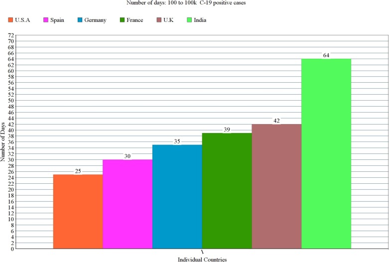
On 19 May 2020, the number of 2019-nCoV cases in India crossed the 100 k mark, almost four months after the country reported its first 2019-nCoV infection. But India’s 2019-nCoV growth rate has been much slower compared with some of the seriously affected countries of the world. According to data compiled by the family health and welfare ministry, it took 64 days for the number of 2019-nCoV cases to rise from 100 to 100 K in India (Fig. 1 ).

Fig. 1.

From 100 to 100K mark 2019-nCoV cases.

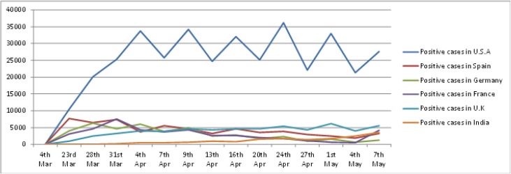
It took 25 days for the infections to grow from 100 to 100 K mark cases in the United States, the country with the highest number of cases worldwide. So far, the world has recorded $\sim$1.4 million infections per lakh population, average about 431. Italy, with the highest number of 2019-nCoV deaths reported in Europe, saw its 2019-nCoV count go from 100 to 100 K in 36 days. It currently has $\sim$2.24 lakh cases, with 372 infections per lakh population averaging. Similarly, after recording 100 cases in 42 days, UK crossed the one-lakh mark. The country has $\sim$2.4 lakh cases reported so far, with an estimated average of 361 infections per lakh population. France, which identified $\sim$1.4 lakh cases and has approximately 209 cases per lakh population, has seen its 2019-nCoV count in 39 days go from 100 to one lakh. Although it took 35 days for cases to increase from 100 to 1 lakh in Germany, which has reported $\sim$1.7 lakh infections and 210 cases per lakh population. In Spain, climbing from 100 to 100 K took 30 days for the cases. After Italy, the European nation was the second most horribly hit nation in Europe and registered $\sim$2.3 lakh infections of 2019-nCoV, resulting in around 494 cases per lakh population (see Fig. 2 for more info).

Fig. 2.

The comparison between Cases of Covid-19 and different countries.

According to data from the WHO, more than 4.5 million cases of 2019-nCoV were registered globally before 18th May 2020, which is around 60 cases per lakh population. China implemented and/or followed strict rules and regulations to defeat 2019-nCoV. When 2019-nCoV outbreaks escalated in Wuhan, China, in late February, officials went house-to house for medical examinations-forcefully isolating every person in informal hospitals and provisional quarantine centers, including extracting parents from small children who exhibited signs of 2019-nCoV, no matter how mild it might be. Healthcare professionals at the omnipresent big apartment buildings in the city were forced into action as asynchronous security officers, tracking the temperatures of all occupants, determining who could join and carrying out assessments of distributed feed ingredients and medicines. There, drones circled over the sidewalks, shouting at citizens to get inside and haranguing them for not wearing surgical masks, whilst elsewhere in China face detection tech, connected to a compulsory phone app that color-coded people based on their contagion danger, determined who should go into shopping malls, subway stations, restaurants and other public areas. We may conclude that this strict rules and regulations prevented spread of 2019-nCoV and hence China is not yet touched the mark 100 K novel strain coronavirus cases even though it has first outbreak escalated in China.

How China was able to flatten the curve compared to other nations?

Additional travel restrictions ($\sim 90\%$ of traffic) have only a marginal impact when combined with public safety measures and behavioural improvements that can promote a substantial reduction in the transmissibility of diseases. The 2019-nCoV pandemic is currently causing havoc throughout the world, handling a devastating blast to countries with a few of the world’s best health services. Though the West has not been able to handle the 2019-nCoV pandemic adequately thus far, China, Singapore, Taiwan and Thailand have taught the world how to control this extremely contagious epidemic. Although China initially botched up, its answer to 2019-nCoV rapidly adapted and improvised. Even when their response initially seemed intrusive, it was probably the only way left for the country in retrospect.

Here are the some main factors influenced the China to control the 2019-nCoV:

• •Creating and maintaining a no-travel regions and prohibiting people from entering or leaving this regions, limiting infection spread to the rest.
• •Suspending schools and places of employment after January 26th 2020, leading to a drastic decline in new infections.
• •Continuing to make testing of the coronavirus free and easy to access.
• •Extensive contact monitoring of peoples who might have met patients with novel strain coronavirus 2019-nCoV/SARS-CoV-2.
• •Establish transitional health centers, and employ 40 K health care professionals from other provinces.
• •In time supply of medical kits, food and groceries to the needy.
• •Mindfulness campaigns demanding that people always wear a mask.
• •Implementing within country travel ban and International travel ban.

Since around 27th May,2020, the total number of cases of coronavirus in China was 82,891 and the total number of deaths was 4634 and its recovery rate is $\sim 91\%$. Below Fig. 3 represents the graphical view of flatten curve against covid-19 cases. For more info, the reader can refer to [21].

Fig. 3.

Flatten curve against covid-19 cases.

Reproduction number($R_0$) of the 2019-nCoV

A set of major components describe the trajectory of an outbreak, some of which actually remain poorly known for COVID-19. The standard reproduction number($R_0$), which characterizes the average number of associated cases produced by one initial case where the community is large part susceptible to infection, helps determine the total number of people likely to be contaminated or, more exactly, the region under the outbreak trajectory. The importance of $R_0$ must be greater than equality in meaning for an outbreak to take hold. A straightforward estimate provides the fraction without containment likely to get infected. The fraction is around $1-\frac{1}{R_0}$.

In China, COVID-19 about 2.5 in the early stages of the disease, and estimated that around 60$\%$ of the population will become contaminated. For a variety of factors, that’s a really bad case situation. We’re uncertain about infant transfer, several societies are voluntary social distancing by persons and groups would have an effect internally and unlikely to be revealed, and preventive initiatives, such as the steps placed in China, would significantly minimize transmission. As an outbreak develops, the cumulative reproduction number ($R_0$) drops until it falls under equilibrium in value as the disease occurs and then declines, either due to the depletion of individuals susceptible to contamination or the impact of prevention steps. The rate of the preliminary progression of the disease, its subsequent improvement, or the associated sequential period (the duration it takes for an infectious person to transmit the Infection with others) and the possible length of the outbreak are calculated by variables such as the period of the infection, and the mean contagious period. A new study[22] indicates that the $R_0$ of extreme acute respiratory coronavirus syndrome (SARS-CoV-2) could be as high as 5.7, up from the original estimate $R_0$ of 2.28 (according to [23]). These studies often tend to presume uniform pathogenicity and virus propagation over time, and do not account for virus mutation either to or away from a more virulent strain (Fig. 4 ).

Fig. 4.

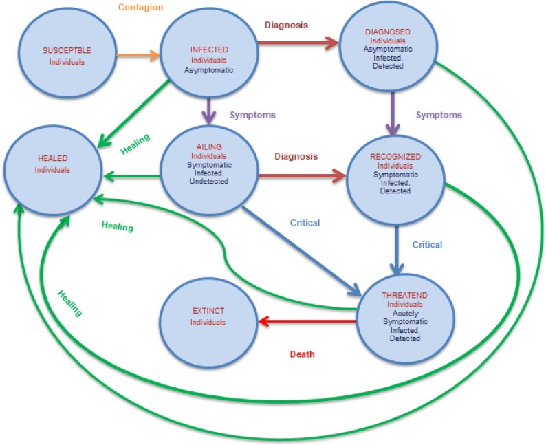
Graphical scheme describing the connections in the mathematical model SIDARTHE between various phases of the infection.

Discussion and results on existing mathematical models of the 2019-nCoV

Infectious diseases continue to exist as one of the main sources of death around the world (adding to 26% of worldwide mortality in 2001; WHO, 2002). With the sudden increase in occurrences of a SARS-CoV in 2003, Mers-CoV in 2012, Ebola in 2014 and now SARS-CoV-2: expanding worries about natural psychological warfare and/or increasing concerns about biological violence, epidemic modelling has taken on a much important to be worthy of role for strategy making from a public health viewpoint. Mathematical and/or scientific models of infectious diseases can help us to interpret disease dynamics and transmission rate. Models also allow us to permit us to re-enact the spread of diseases in various prospects and aspects in order to develop and assess various intervention methodologies to forestall or enhance contaminations and better allot accessible resources (for example, choosing the target population, time for intervention and the location). Predictive mathematical models are important for predicting the progression of the outbreak and for preparing successful response strategies. The human-to-human transmission SIR model, which defines people’s movement across three mutually incompatible periods of infection: susceptible, infected, and recovered. More complex models can depict precisely the diverse propagation of particular infectious diseases. Several models had been developed for the 2019-nCoV pandemic. Another widely applied framework is: Lin et al., extended an SEIR model (susceptible, exposed, infectious, removed), taking into account the understanding of threat and the cumulative number of cases.

Now, it is worthy to mention that some recent developments in mathematical models pertinent to the 2019-nCoV:

• •
  Altaf and Atangana[4] suggested a mathematical model of type SEIARM and it is able to depict the spread of the 2019-nCoV as follows:

  $$\left(\begin{array}{cc}\hfill & \frac{d{\mathcal{S}}_p}{d\theta }={\mathrm{\Pi }}_p-a_p{\mathcal{S}}_p-\frac{b_p{\mathcal{S}}_p({\mathcal{I}}_p+\mathrm{\Psi }{\mathcal{A}}_p)}{{\mathcal{N}}_p}-b_w{\mathcal{S}}_p\mathcal{M}\text{;}\hfill \\ \hfill & \frac{d{\mathcal{E}}_p}{d\theta }=\frac{b_p{\mathcal{S}}_p({\mathcal{I}}_p+\mathrm{\Psi }{\mathcal{A}}_p)}{{\mathcal{N}}_p}+b_w{\mathcal{S}}_p\mathcal{M}-(1-{\mathrm{\Upsilon }}_p){\omega }_p{\mathcal{E}}_p-{\mathrm{\Upsilon }}_p{\xi }_p{\mathcal{E}}_p-a_p{\mathcal{E}}_p\text{;}\hfill \\ \hfill & \frac{d{\mathcal{I}}_p}{d\theta }=(1-{\mathrm{\Upsilon }}_p){\omega }_p{\mathcal{E}}_p-({\tau }_p+a_p){\mathcal{I}}_p\text{;}\hfill \\ \hfill & \frac{d{\mathcal{A}}_p}{d\theta }={\mathrm{\Upsilon }}_p{\xi }_p{\mathcal{E}}_p-({\tau }_{\vartheta p}+a_p){\mathcal{A}}_p\text{;}\hfill \\ \hfill & \frac{d{\mathcal{R}}_p}{d\theta }={\tau }_p{\mathcal{I}}_p+{\tau }_{\vartheta p}{\mathcal{A}}_p-a_p{\mathcal{R}}_p\text{;}\hfill \\ \hfill & \frac{d\mathcal{M}}{d\theta }=c_p{\mathcal{I}}_p+e_p{\mathcal{A}}_p-\pi \mathcal{M}\text{.}\hfill \end{array}\right\}$$ (1)

  More importantly they suggested using some collected data a reproductive number$(R_0)$ about 2.4, which was in good agreement with the value suggested by WHO. The fractional model is then numerically overcome by showing several graphical data, which will further mitigate the infection. For more information pertinent to this model and mathematical terminology the reader can refer to Fig. 5 as well as [4].

• •To curtail the global spread of the 2019-nCoV needs several population-wide interventions to be implemented; nevertheless, it remains unclear whether the pacing and rigor of these steps would impact ’flattening the curve’. Very recently, Giulia Giordano et al. [5], developed a new model that correctly predicted the transformation of epidemics and assist to identify the effect of various strategies to contain the transmission of infection, such as lock-down and social distance, along with testing and contact transmitting. The model takes into account 8 levels of infection: susceptible (S), infected(I), diagnosed (D), ailing (A), recognized (R), threatened (T), healed (H) and extinct (E), collectively called SIDARTHE. See the diagrammatic representation of SIDARTHE model in Fig. 6 . The central claim of this model is the correlation amongst cases of observed and unnoticed transmission, and cases with separate classifications of SOIs (mild and moderate vs major and severe). Making a distinction between medicated and unmedicated cases enables us to underline the presumed distortion in statistics on diseases, such as the number of infected persons, transmission rate and CFR (ratio of the number of fatalities and number of confirmed cases related to the infection). In addition, this model helps to analyze and understand the impact of implementing various guidelines and regulations (e.g., more substantial disease confirmatory testing or more stringent social distance measures), typically resulting in a change in model parameters. The model aims to analyse and understand the impact of implementing the Various recommendations and procedures (For e.g., more comprehensive disease monitoring or more rigorous social isolation precautions), usually contributing to a shift in simulation results.
• •In [6], findings claimed a mathematical model-SCIRD that would take into consideration the lock-down effect and the possibility of transmission from deceased to susceptible individuals as well. Suffice it to say, the model doesn’t collect all the information into consideration the spread, nor is the model a solution for COVID-19, but the model is intended to affirm or dismiss the impact of lock-down as a potentially appropriate step to better flatten the death and infection curves.

Fig. 5.

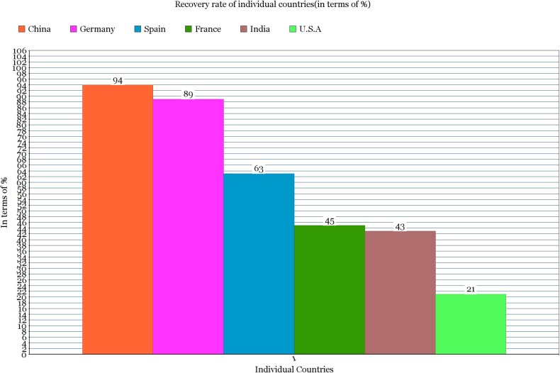
Recovery rate against individual countries.

Fig. 6.

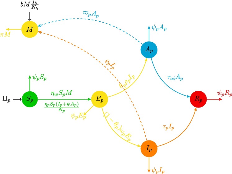
Interaction among the people and the reservoir (seafood) market.

It is therefore important to note, there is a drastic increase for utilizing mathematical modeling in the study of epidemiology diseases. Mathematical models also used for identifying/estimating various diseases growth and/or abnormal growth of tissue-resistant to a particular infection surveillance natural phenomena procedures(see for example [7], [8], [9], [10], [11]).

Results on fractional models of 2019-nCoV

Definition 5.1

[12] Let $(X,d)$ be complete metric space. A mapping $\mathcal{O}:X\to X$ is said to be a $(\xi -\mathcal{F})$-contraction, if there exist the functions $\mathcal{F}:(0,\infty )\to \mathbb{R}$ and $\xi :(0,\infty )\to (0,\infty )$ satisfying:

• $(C_1)$. $\mathcal{F}$ satisfies $({\mathfrak{C}}^{\ast }),({\mathfrak{C}}^{♢})$ and $({\mathfrak{C}}^{\prime })$;

• $(C_2)$. $\lim {\inf }_{s\to x^{+}}\xi (s)>0$ for all $x⩾0$;

• $(C_3)$. $\xi (d(x,y))+\mathcal{F}(d(\mathcal{O}x,\mathcal{O}y))⩽\mathcal{F}(d(x,y))$

where,

• $({\mathfrak{C}}^{\ast })$. F is strictly increasing;

• $({\mathfrak{C}}^{♢})$. There exists $k\in (0,1)$ such that ${\lim }_{\theta \to 0^{+}}{\theta }^{k}F(\theta )=0$;

• $({\mathfrak{C}}^{\prime })$. ${\lim }_{\theta \to 0^{+}}F(\theta )=-\infty$;

for all $x,y\in X$ such that $\mathcal{O}x\ne \mathcal{O}y$.

Theorem 5.1

[12] Let $(X,d)$ be a complete metric space and let $\mathcal{O}:X\to X$ be a $(\xi -\mathcal{F})$ -contraction and for each $x_0\in X$ . Then $\mathcal{O}$ has a unique fixed point.

This topic $(\xi -\mathcal{F})$-contraction is an extension of F-contraction. Any traditional discussions indicate that literature on this topic may infer that the concept of F-contraction is a typical generalization of the Banach contraction principle as a consequence of the uniqueness. For a extensive study on fixed points,F-contraction and fractionals the reader may refer [13], [14], [15], [16], [17], [18], [19], [20], [21], [22], [23], [24], [25], [26], [27], [28], [29], [30], [31], [32], [33], [34].

The 2019-nCoV model of type SEIARM via fractional integral for Mittag-Leffler kernel

We present the existence of fixed point for $(\xi -\mathcal{F})$-contractions to the following 2019-nCoV model of type SEIARM.

$$\left(\begin{array}{cc}\hfill & {\mathcal{S}}_p(\theta )-{\mathcal{S}}_p(0)=\frac{1-\alpha }{C_{19}(\alpha )}\mathbb{A}(\theta ,{\mathcal{S}}_p)+\frac{\alpha }{C_{19}(\alpha )\mathrm{\Gamma }(\alpha )}{\int }_0^{\theta }\mathbb{A}(\nu ,{\mathcal{S}}_p){(\theta -\nu )}^{\alpha -1}d\nu \hfill \\ \hfill & {\mathcal{E}}_p(\theta )-{\mathcal{E}}_p(0)=\frac{1-\alpha }{C_{19}(\alpha )}\mathbb{B}(\theta ,{\mathcal{S}}_p)+\frac{\alpha }{C_{19}(\alpha )\mathrm{\Gamma }(\alpha )}{\int }_0^{\theta }\mathbb{B}(\nu ,{\mathcal{S}}_p){(\theta -\nu )}^{\alpha -1}d\nu \hfill \\ \hfill & {\mathcal{I}}_p(\theta )-{\mathcal{I}}_p(0)=\frac{1-\alpha }{C_{19}(\alpha )}\mathbb{C}(\theta ,{\mathcal{S}}_p)+\frac{\alpha }{C_{19}(\alpha )\mathrm{\Gamma }(\alpha )}{\int }_0^{\theta }\mathbb{C}(\nu ,{\mathcal{S}}_p){(\theta -\nu )}^{\alpha -1}d\nu \hfill \\ \hfill & {\mathcal{A}}_p(\theta )-{\mathcal{A}}_p(0)=\frac{1-\alpha }{C_{19}(\alpha )}\mathbb{D}(\theta ,{\mathcal{S}}_p)+\frac{\alpha }{C_{19}(\alpha )\mathrm{\Gamma }(\alpha )}{\int }_0^{\theta }\mathbb{D}(\nu ,{\mathcal{S}}_p){(\theta -\nu )}^{\alpha -1}d\nu \hfill \\ \hfill & {\mathcal{R}}_p(\theta )-{\mathcal{R}}_p(0)=\frac{1-\alpha }{C_{19}(\alpha )}\mathbb{E}(\theta ,{\mathcal{S}}_p)+\frac{\alpha }{C_{19}(\alpha )\mathrm{\Gamma }(\alpha )}{\int }_0^{\theta }\mathbb{E}(\nu ,{\mathcal{S}}_p){(\theta -\nu )}^{\alpha -1}d\nu \hfill \\ \hfill & {\mathcal{M}}_p(\theta )-{\mathcal{M}}_p(0)=\frac{1-\alpha }{C_{19}(\alpha )}\mathbb{F}(\theta ,{\mathcal{S}}_p)+\frac{\alpha }{C_{19}(\alpha )\mathrm{\Gamma }(\alpha )}{\int }_0^{\theta }\mathbb{F}(\nu ,{\mathcal{S}}_p){(\theta -\nu )}^{\alpha -1}d\nu \hfill \\ \hfill \end{array}\right\}$$ (2)

Here we prove the existence and unique solution of the 2019-nCoV model of type SEIARM.

Consider the Banach space $\mathcal{C}(I)$ of all continuous functions $x:I\to \mathbb{R}$ equipped with Bielecki’s norm

$$||x||={\displaystyle \underset{\theta \in I}{\sup }}{e}^{-\theta }|x(\theta )|$$

In order to prove our Theorem, above stated theorem plays a vital role. Moreover, we need the following assumptions:

• $({\mathcal{H}}_1)$. $\lim \underset{a\to {\theta }^{+}}{\inf }\xi (a)>0\mathrm{for}\mathrm{all}t⩾0$;

• $({\mathcal{H}}_2)$. $\frac{(1-\alpha )\mathrm{\Gamma }(\alpha )+{\theta }^e}{C_{19}(\alpha )\mathrm{\Gamma }(\alpha )}<\frac{{\sigma }_n}{{\sigma }_{n+1}(1+{\sigma }_n({\sigma }_n-{\sigma }_{n-1}))}{e}^{-\theta {\sigma }_n}$;

• $({\mathcal{H}}_3)$. $\mathbb{A}(\theta ,{\mathcal{S}}_{p_1})-\mathbb{A}(\theta ,{\mathcal{S}}_{p_2})|<|{\mathcal{S}}_{p_1}(\theta )-{\mathcal{S}}_{p_2}(\theta )|$.

Theorem 5.2

If ${\mathcal{H}}_1,{\mathcal{H}}_2$ and ${\mathcal{H}}_3$ satisfied, then the 2019-nCoV model of type SEIARM has a unique solution in $\mathcal{C}(I)$ .

Proof. Consider the operator $\mathcal{O}:\mathcal{C}(I)\to \mathcal{C}(I)$ as follows,

$${\mathcal{OS}}_p(\theta )={\mathcal{S}}_p(0)=\frac{1-\alpha }{C_{19}(\alpha )}\mathbb{A}(\theta ,{\mathcal{S}}_p)+\frac{\alpha }{C_{19}(\alpha )\mathrm{\Gamma }(\alpha )}{\int }_0^{\theta }\mathbb{A}(\nu ,{\mathcal{S}}_p){(\theta -\nu )}^{\alpha -1}d\nu \text{;}{\mathcal{S}}_p\in \mathcal{C}(I)\text{.}$$ (3)

A fixed point of the operator $\mathcal{O}$ will be a solution of Eq. (2). In order to fulfil all the assumptions of Theorem 5.1, let us consider a function $\mathcal{F}(x)=-\frac{1}{x},x>0$ and $\xi :(0,\infty )\to (0,\infty )$ of the form:

$$\xi (x)=\left\{\begin{array}{c}-x+{\sigma }_1,0<x<{\sigma }_1\hfill \\ -x+{\sigma }_n,{\sigma }_{n-1}⩽x<{\sigma }_n,n⩾2\hfill \end{array}\right)$$

In this case one can calculate that the contractive condition takes the following form:

$$\xi (d(x,y))+\mathcal{F}(d(\mathcal{O}x,\mathcal{O}y))⩽\mathcal{F}(d(x,y))$$

$$\Rightarrow -d(x,y)+{\sigma }_n+\mathcal{F}(d(\mathcal{O}x,\mathcal{O}y))⩽\mathcal{F}(d(x,y))$$

$$\Rightarrow -||x-y||+{\sigma }_n+\mathcal{F}(||\mathcal{O}x-\mathcal{O}y||)⩽\mathcal{F}(||x-y||)$$

$$\Rightarrow {\sigma }_n-||x-y||-\frac{1}{||\mathcal{O}x-\mathcal{O}y||}⩽-\frac{1}{||x-y||}$$

$$\Rightarrow {\sigma }_n-||x-y||-\frac{1}{||x-y||}⩽\frac{1}{||\mathcal{O}x-\mathcal{O}y||}$$

$$\Rightarrow \frac{[{\sigma }_n-||x-y||]||x-y||+1}{||x-y||}⩽\frac{1}{||\mathcal{O}x-\mathcal{O}y||}$$

$$\Rightarrow ||\mathcal{O}x-\mathcal{O}y||⩽\frac{||x-y||}{[{\sigma }_n-||x-y||]||x-y||+1}$$

for all $x,y\in \mathcal{C}(I)$ satisfying ${\sigma }_{n-1}⩽||x-y||<{\sigma }_n$ when $n⩾2$ and $0<||x-y||<{\sigma }_1$ for $n=1$. We will show that $\mathcal{O}$ satisfies the conditions of Theorem 5.1. Fix $n⩾2$ and take any $\mathbb{A}(\nu ,{\mathcal{S}}_{p_1}),\mathbb{A}(\nu ,{\mathcal{S}}_{p_2})\in \mathcal{C}(I)$ such that ${\sigma }_{n-1}⩽||x-y||<{\sigma }_n$. Observe that for each $\nu \in I$, we have,

$$\mathbb{A}(\nu ,{\mathcal{S}}_{p_1})-\mathbb{A}(\nu ,{\mathcal{S}}_{p_2})⩽e^{\nu }{\displaystyle \underset{\nu \in I}{\sup }}{e}^{-\nu }$$

$$\mathbb{A}(\nu ,{\mathcal{S}}_{p_1})-\mathbb{A}(\nu ,{\mathcal{S}}_{p_2})⩽e^{\nu }{\sigma }_n⩽e^{\theta }{\sigma }_n$$

Consider,

$$\begin{array}{cc}|{\mathcal{OS}}_{p_1}(\theta )-{\mathcal{OS}}_{p_2}(\theta )|\hfill & =|\frac{1-\alpha }{C_{19}(\alpha )}\mathbb{A}(\theta ,{\mathcal{S}}_{p_1})+\frac{\alpha }{C_{19}(\alpha )\mathrm{\Gamma }(\alpha )}{\int }_0^{\theta }\mathbb{A}(\nu ,{\mathcal{S}}_{p_1}){(\theta -\nu )}^{\alpha -1}d\nu \hfill \\ \hfill & -\frac{1-\alpha }{C_{19}(\alpha )}\mathbb{A}(\theta ,{\mathcal{S}}_{p_2})-\frac{\alpha }{C_{19}(\alpha )\mathrm{\Gamma }(\alpha )}{\int }_0^{\theta }\mathbb{A}(\nu ,{\mathcal{S}}_{p_2}){(\theta -\nu )}^{\alpha -1}d\nu |\hfill \\ \hfill & ⩽|\frac{1-\alpha }{C_{19}(\alpha )}||\mathbb{A}(\theta ,{\mathcal{S}}_{p_1})-\mathbb{A}(\theta ,{\mathcal{S}}_{p_2})|\hfill \\ \hfill & +|\frac{\alpha }{C_{19}(\alpha )\mathrm{\Gamma }(\alpha )}||{\int }_0^{\theta }{(\theta -\nu )}^{\alpha -1}d\nu ||\mathbb{A}(\theta ,{\mathcal{S}}_{p_1})-\mathbb{A}(\theta ,{\mathcal{S}}_{p_2})|\hfill \\ \hfill & ⩽|\frac{1-\alpha }{C_{19}(\alpha )}||\mathbb{A}(\theta ,{\mathcal{S}}_{p_1})-\mathbb{A}(\theta ,{\mathcal{S}}_{p_2})|\hfill \\ \hfill & +|\frac{\alpha }{C_{19}(\alpha )\mathrm{\Gamma }(\alpha )}||\mathbb{A}(\theta ,{\mathcal{S}}_{p_1})-\mathbb{A}(\theta ,{\mathcal{S}}_{p_2})||{\left(\frac{{(\theta -\nu )}^{\alpha }}{\alpha }\right)}_0^{\theta }|\hfill \\ \hfill & ⩽|\mathbb{A}(\theta ,{\mathcal{S}}_{p_1})-\mathbb{A}(\theta ,{\mathcal{S}}_{p_2})||\frac{1-\alpha }{C_{19}(\alpha )}+\frac{{\theta }^{\alpha }}{C_{19}(\alpha )\mathrm{\Gamma }(\alpha )}|\hfill \\ \hfill & ⩽|\mathbb{A}(\theta ,{\mathcal{S}}_{p_1})-\mathbb{A}(\theta ,{\mathcal{S}}_{p_2})||\frac{(1-\alpha )\mathrm{\Gamma }(\alpha )+{\theta }^{\alpha }}{C_{19}(\alpha )\mathrm{\Gamma }(\alpha )}|e^{-\theta {\sigma }_{n+1}}{e}^{\theta {\sigma }_{n+1}}\hfill \\ \hfill & ⩽|\mathbb{A}(\theta ,{\mathcal{S}}_{p_1})-\mathbb{A}(\theta ,{\mathcal{S}}_{p_2})|\frac{{\sigma }_n}{{\sigma }_{n+1}(1+{\sigma }_n({\sigma }_n-{\sigma }_{n-1}))}{e}^{-\theta {\sigma }_n}{e}^{-\theta {\sigma }_{n+1}}{e}^{\theta {\sigma }_{n+1}}\hfill \end{array}$$ (4)

Next, we have,

$$\begin{array}{cc}1+||{\mathcal{S}}_{p_1}-{\mathcal{S}}_{p_2}||({\sigma }_n-||{\mathcal{S}}_{p_1}-{\mathcal{S}}_{p_2}||)\hfill & <1+{\sigma }_n({\sigma }_n-{\sigma }_{n-1})\hfill \\ \hfill & ⩽|\mathbb{A}(\theta ,{\mathcal{S}}_{p_1})-\mathbb{A}(\theta ,{\mathcal{S}}_{p_2})|\frac{{\sigma }_n}{(1+||{\mathcal{S}}_{p_1}-{\mathcal{S}}_{p_2}||({\sigma }_n-||{\mathcal{S}}_{p_1}-{\mathcal{S}}_{p_2}||)){\sigma }_{n+1}}\hfill \\ \hfill & \times e^{-\theta {\sigma }_n}{e}^{-\theta {\sigma }_{n+1}}{e}^{\theta {\sigma }_{n+1}}\hfill \end{array}$$ (5)

and since ${\sigma }_{n+1}>1,-\nu {\sigma }_{n+1}⩽-\nu$ for all $\nu \in I$. In consequence, the following holds:

$$\begin{array}{cc}|{\mathcal{OS}}_{p_1}(\theta )-{\mathcal{OS}}_{p_2}(\theta )|\hfill & ⩽|\mathbb{A}(\theta ,{\mathcal{S}}_{p_1})-\mathbb{A}(\theta ,{\mathcal{S}}_{p_2})|\frac{{\sigma }_n}{(1+||{\mathcal{S}}_{p_1}-{\mathcal{S}}_{p_2}||({\sigma }_n-||{\mathcal{S}}_{p_1}-{\mathcal{S}}_{p_2}||)){\sigma }_{n+1}}{e}^{-\theta {\sigma }_{n+1}}{e}^{\theta ({\sigma }_{n+1}-{\sigma }_n)}\hfill \\ \hfill & <\frac{{\sigma }_n||{\mathcal{S}}_{p_1}(\theta )-{\mathcal{S}}_{p_2}(\theta )||}{(1+||{\mathcal{S}}_{p_1}-{\mathcal{S}}_{p_2}||({\sigma }_n-||{\mathcal{S}}_{p_1}-{\mathcal{S}}_{p_2}||)){\sigma }_{n+1}}{e}^{\theta ({\sigma }_{n+1}-{\sigma }_n)}\hfill \end{array}$$ (6)

Using the properties of the sequence $({\sigma }_n)$, we get,

$$e^{-\theta }|{\mathcal{OS}}_{p_1}(\theta )-{\mathcal{OS}}_{p_2}(\theta )|⩽\frac{||{\mathcal{S}}_{p_1}(\theta )-{\mathcal{S}}_{p_2}(\theta )||}{1+||{\mathcal{S}}_{p_1}(\theta )-{\mathcal{S}}_{p_2}(\theta )||({\sigma }_n-||{\mathcal{S}}_{p_1}(\theta )-{\mathcal{S}}_{p_2}(\theta )||)}$$ (7)

By following the same pattern as above, we get,

$$e^{-\theta }|{\mathcal{OE}}_{p_1}(\theta )-{\mathcal{OE}}_{p_2}(\theta )|⩽\frac{||{\mathcal{E}}_{p_1}(\theta )-{\mathcal{E}}_{p_2}(\theta )||}{1+||{\mathcal{E}}_{p_1}(\theta )-{\mathcal{E}}_{p_2}(\theta )||({\sigma }_n-||{\mathcal{E}}_{p_1}(\theta )-{\mathcal{E}}_{p_2}(\theta )||)}$$ (8)

$$e^{-\theta }|{\mathcal{OI}}_{p_1}(\theta )-{\mathcal{OI}}_{p_2}(\theta )|⩽\frac{||{\mathcal{I}}_{p_1}(\theta )-{\mathcal{I}}_{p_2}(\theta )||}{1+||{\mathcal{I}}_{p_1}(\theta )-{\mathcal{I}}_{p_2}(\theta )||({\sigma }_n-||{\mathcal{I}}_{p_1}(\theta )-{\mathcal{I}}_{p_2}(\theta )||)}$$ (9)

$$e^{-\theta }|{\mathcal{OA}}_{p_1}(\theta )-{\mathcal{OA}}_{p_2}(\theta )|⩽\frac{||{\mathcal{A}}_{p_1}(\theta )-{\mathcal{A}}_{p_2}(\theta )||}{1+||{\mathcal{A}}_{p_1}(\theta )-{\mathcal{A}}_{p_2}(\theta )||({\sigma }_n-||{\mathcal{A}}_{p_1}(\theta )-{\mathcal{A}}_{p_2}(\theta )||)}$$ (10)

$$e^{-\theta }|{\mathcal{OR}}_{p_1}(\theta )-{\mathcal{OR}}_{p_2}(\theta )|⩽\frac{||{\mathcal{R}}_{p_1}(\theta )-{\mathcal{R}}_{p_2}(\theta )||}{1+||{\mathcal{R}}_{p_1}(\theta )-{\mathcal{R}}_{p_2}(\theta )||({\sigma }_n-||{\mathcal{R}}_{p_1}(\theta )-{\mathcal{R}}_{p_2}(\theta )||)}$$ (11)

$$e^{-\theta }|{\mathcal{OM}}_{p_1}(\theta )-{\mathcal{OM}}_{p_2}(\theta )|⩽\frac{||{\mathcal{M}}_{p_1}(\theta )-{\mathcal{M}}_{p_2}(\theta )||}{1+||{\mathcal{M}}_{p_1}(\theta )-{\mathcal{M}}_{p_2}(\theta )||({\sigma }_n-||{\mathcal{M}}_{p_1}(\theta )-{\mathcal{M}}_{p_2}(\theta )||)}$$ (12)

Thus, $\mathcal{O}$ gratified all the conditions of the above Theorem 5.1. Hence $\mathcal{O}$ has a fixed point which yields a solution which gives the existence of solution for 2019-nCoV model of type SEIARM.

The 2019-nCoV model of type SCIRD via fractal-fractional integral for Mittag-Leffler kernel

In this section, we consider,

$$\begin{array}{cc}{}_0^{\mathit{FFM}}{D}_{\theta }^{\alpha ,\beta }\hfill & y(\theta )=g(\theta ,y(\theta ))\hfill \\ \hfill & y(0)=y_0\hfill \end{array}$$ (13)

Applying the fractal-fractional integral with Mittag-Leffler kernel according to [6], we transform the above equation into

$$y(\theta )=y(0)+\frac{1-\alpha }{C_{19}(\alpha )}{\theta }^{1-\beta }g(\theta ,y(\theta ))+\frac{\alpha }{C_{19}(\alpha )\mathrm{\Gamma }(\alpha )}{\int }_0^{\theta }g(\psi ,y(\psi )){(\theta -\psi )}^{\alpha -1}{\psi }^{1-\beta }d\psi$$ (14)

Below is the 2019-nCoV model of type SCIRD associated with fractal-fractional integral with Mittag-Leffler kernel:

$$\left(\begin{array}{cc}\hfill & \mathcal{S}(\theta )=\mathcal{S}(0)+\frac{1-\alpha }{C_{19}(\alpha )}{\theta }^{1-\beta }\mathcal{A}(\theta ,\mathcal{S}(\theta ),\mathcal{C}(\theta ),\mathcal{I}(\theta ),\mathcal{R}(\theta ),\mathcal{D}(\theta ))\hfill \\ \hfill & +\frac{\alpha }{C_{19}(\alpha )\mathrm{\Gamma }(\alpha )}{\int }_0^{\theta }\mathcal{A}(\psi ,\mathcal{S}(\psi ),\mathcal{C}(\psi ),\mathcal{I}(\psi ),\mathcal{R}(\psi ),\mathcal{D}(\psi )){\psi }^{1-\beta }{(\theta -\psi )}^{\alpha -1}d\psi \hfill \\ \hfill & \mathcal{C}(\theta )=\mathcal{C}(0)+\frac{1-\alpha }{C_{19}(\alpha )}{\theta }^{1-\beta }\mathcal{B}(\theta ,\mathcal{S}(\theta ),\mathcal{C}(\theta ),\mathcal{I}(\theta ),\mathcal{R}(\theta ),\mathcal{D}(\theta ))\hfill \\ \hfill & +\frac{\alpha }{C_{19}(\alpha )\mathrm{\Gamma }(\alpha )}{\int }_0^{\theta }\mathcal{B}(\psi ,\mathcal{S}(\psi ),\mathcal{C}(\psi ),\mathcal{I}(\psi ),\mathcal{R}(\psi ),\mathcal{D}(\psi )){\psi }^{1-\beta }{(\theta -\psi )}^{\alpha -1}d\psi \hfill \\ \hfill & \mathcal{I}(\theta )=\mathcal{I}(0)+\frac{1-\alpha }{C_{19}(\alpha )}{\theta }^{1-\beta }\mathcal{C}(\theta ,\mathcal{S}(\theta ),\mathcal{C}(\theta ),\mathcal{I}(\theta ),\mathcal{R}(\theta ),\mathcal{D}(\theta ))\hfill \\ \hfill & +\frac{\alpha }{C_{19}(\alpha )\mathrm{\Gamma }(\alpha )}{\int }_0^{\theta }\mathcal{C}(\psi ,\mathcal{S}(\psi ),\mathcal{C}(\psi ),\mathcal{I}(\psi ),\mathcal{R}(\psi ),\mathcal{D}(\psi )){\psi }^{1-\beta }{(\theta -\psi )}^{\alpha -1}d\psi \hfill \\ \hfill & \mathcal{R}(\theta )=\mathcal{R}(0)+\frac{1-\alpha }{C_{19}(\alpha )}{\theta }^{1-\beta }\mathcal{D}(\theta ,\mathcal{S}(\theta ),\mathcal{C}(\theta ),\mathcal{I}(\theta ),\mathcal{R}(\theta ),\mathcal{D}(\theta ))\hfill \\ \hfill & +\frac{\alpha }{C_{19}(\alpha )\mathrm{\Gamma }(\alpha )}{\int }_0^{\theta }\mathcal{D}(\psi ,\mathcal{S}(\psi ),\mathcal{C}(\psi ),\mathcal{I}(\psi ),\mathcal{R}(\psi ),\mathcal{D}(\psi )){\psi }^{1-\beta }{(\theta -\psi )}^{\alpha -1}d\psi \hfill \\ \hfill & \mathcal{D}(\theta )=\mathcal{D}(0)+\frac{1-\alpha }{C_{19}(\alpha )}{\theta }^{1-\beta }\mathcal{E}(\theta ,\mathcal{S}(\theta ),\mathcal{C}(\theta ),\mathcal{I}(\theta ),\mathcal{R}(\theta ),\mathcal{D}(\theta ))\hfill \\ \hfill & +\frac{\alpha }{C_{19}(\alpha )\mathrm{\Gamma }(\alpha )}{\int }_0^{\theta }\mathcal{E}(\psi ,\mathcal{S}(\psi ),\mathcal{C}(\psi ),\mathcal{I}(\psi ),\mathcal{R}(\psi ),\mathcal{D}(\psi )){\psi }^{1-\beta }{(\theta -\psi )}^{\alpha -1}d\psi \hfill \\ \hfill \end{array}\right\}$$ (15)

We apply Theorem 5.1 to verify the existence problems of the unique solutions for Mittag-Leffler Kernal Covid model. We look for the solution of Eq. (15) in a subset $\mathcal{C}$ of the Banach space X of continues functions defined as below equipped with the supremum norm of the form:

$$\mathcal{C}=\{x\in X/{\displaystyle \underset{\theta \in I}{\sup }}{e}^{-\theta }|x(\theta )|\}$$

where $\mathcal{C}(I,X)$ be the Banach space of all continuous functions from I into X.

Here the Bielecki’s norm is defined as:

$$||x||={\displaystyle \underset{\theta \in I}{\sup }}{e}^{-\theta }|x(\theta )|\mathrm{for}x\in \mathcal{C}(I,X)\text{.}$$

In order to obtain our claims, we will need the following assumptions.

• $({\mathcal{Z}}_1)$. ${\mathcal{S}}_1(0)={\mathcal{S}}_2(0)=0$;
• $({\mathcal{Z}}_2)$. $\lim \underset{a\to {\theta }^{+}}{\inf }\xi (a)>0\mathrm{for}\mathrm{all}t⩾0$;
• $({\mathcal{Z}}_3)$. $\frac{{\theta }^{1-\beta }}{C_{19}(\alpha )}\left[1-\alpha +\frac{\alpha {\theta }^{\alpha }\mathrm{\Gamma }(2-\beta )}{\mathrm{\Gamma }(2-\beta +\alpha )}\right]<\frac{{\alpha }_n}{{\alpha }_{n+1}(1+{\alpha }_n({\alpha }_n-{\alpha }_{n-1}))}{e}^{-\theta {\alpha }_n}$;
• $({\mathcal{Z}}_4)$. $|{\mathcal{S}}_1(\theta ,\mathcal{S}(\theta ),\mathcal{C}(\theta ),\mathcal{I}(\theta ),\mathcal{R}(\theta ),\mathcal{D}(\theta ))-{\mathcal{S}}_2(\theta ,\mathcal{S}(\theta ),\mathcal{C}(\theta ),\mathcal{I}(\theta ),\mathcal{R}(\theta ),\mathcal{D}(\theta ))|<|{\mathcal{S}}_1(\theta )-{\mathcal{S}}_2(\theta )|$

Theorem 5.3

If ${\mathcal{Z}}_1,{\mathcal{Z}}_2,{\mathcal{Z}}_3$ and ${\mathcal{Z}}_4$ satisfied, then the 2019-nCoV model of type SCIRD has a unique solution in $\mathcal{C}(I)$ .

Proof. Consider the operator $\mathcal{O}:\mathcal{C}(I,X)\to \mathcal{C}(I,X)$ as follows.

$$\left(\begin{array}{cc}\hfill & \mathcal{OS}(\theta )=\mathcal{S}(0)+\frac{1-\alpha }{C_{19}(\alpha )}{\theta }^{1-\beta }\mathcal{A}(\theta ,\mathcal{S}(\theta ),\mathcal{C}(\theta ),\mathcal{I}(\theta ),\mathcal{R}(\theta ),\mathcal{D}(\theta ))\hfill \\ \hfill & +\frac{\alpha }{C_{19}(\alpha )\mathrm{\Gamma }(\alpha )}{\int }_0^{\theta }\mathcal{A}(\psi ,\mathcal{S}(\psi ),\mathcal{C}(\psi ),\mathcal{I}(\psi ),\mathcal{R}(\psi ),\mathcal{D}(\psi )){\psi }^{1-\beta }{(\theta -\psi )}^{\alpha -1}d\psi \hfill \\ \hfill & \mathcal{OC}(\theta )=\mathcal{C}(0)+\frac{1-\alpha }{C_{19}(\alpha )}{\theta }^{1-\beta }\mathcal{B}(\theta ,\mathcal{S}(\theta ),\mathcal{C}(\theta ),\mathcal{I}(\theta ),\mathcal{R}(\theta ),\mathcal{D}(\theta ))\hfill \\ \hfill & +\frac{\alpha }{C_{19}(\alpha )\mathrm{\Gamma }(\alpha )}{\int }_0^{\theta }\mathcal{B}(\psi ,\mathcal{S}(\psi ),\mathcal{C}(\psi ),\mathcal{I}(\psi ),\mathcal{R}(\psi ),\mathcal{D}(\psi )){\psi }^{1-\beta }{(\theta -\psi )}^{\alpha -1}d\psi \hfill \\ \hfill & \mathcal{OI}(\theta )=\mathcal{I}(0)+\frac{1-\alpha }{C_{19}(\alpha )}{\theta }^{1-\beta }\mathcal{C}(\theta ,\mathcal{S}(\theta ),\mathcal{C}(\theta ),\mathcal{I}(\theta ),\mathcal{R}(\theta ),\mathcal{D}(\theta ))\hfill \\ \hfill & +\frac{\alpha }{C_{19}(\alpha )\mathrm{\Gamma }(\alpha )}{\int }_0^{\theta }\mathcal{C}(\psi ,\mathcal{S}(\psi ),\mathcal{C}(\psi ),\mathcal{I}(\psi ),\mathcal{R}(\psi ),\mathcal{D}(\psi )){\psi }^{1-\beta }{(\theta -\psi )}^{\alpha -1}d\psi \hfill \\ \hfill & \mathcal{OR}(\theta )=\mathcal{R}(0)+\frac{1-\alpha }{C_{19}(\alpha )}{\theta }^{1-\beta }\mathcal{D}(\theta ,\mathcal{S}(\theta ),\mathcal{C}(\theta ),\mathcal{I}(\theta ),\mathcal{R}(\theta ),\mathcal{D}(\theta ))\hfill \\ \hfill & +\frac{\alpha }{C_{19}(\alpha )\mathrm{\Gamma }(\alpha )}{\int }_0^{\theta }\mathcal{D}(\psi ,\mathcal{S}(\psi ),\mathcal{C}(\psi ),\mathcal{I}(\psi ),\mathcal{R}(\psi ),\mathcal{D}(\psi )){\psi }^{1-\beta }{(\theta -\psi )}^{\alpha -1}d\psi \hfill \\ \hfill & \mathcal{OD}(\theta )=\mathcal{D}(0)+\frac{1-\alpha }{C_{19}(\alpha )}{\theta }^{1-\beta }\mathcal{E}(\theta ,\mathcal{S}(\theta ),\mathcal{C}(\theta ),\mathcal{I}(\theta ),\mathcal{R}(\theta ),\mathcal{D}(\theta ))\hfill \\ \hfill & +\frac{\alpha }{C_{19}(\alpha )\mathrm{\Gamma }(\alpha )}{\int }_0^{\theta }\mathcal{E}(\psi ,\mathcal{S}(\psi ),\mathcal{C}(\psi ),\mathcal{I}(\psi ),\mathcal{R}(\psi ),\mathcal{D}(\psi )){\psi }^{1-\beta }{(\theta -\psi )}^{\alpha -1}d\psi \hfill \\ \hfill \end{array}\right\}$$ (16)

A fixed point of the operator $\mathcal{O}$ be a solution of Eq. (15). In order to fulfil all the assumptions of Theorem 5.1, let us consider a function $\mathcal{F}(x)=\log (x)\text{;}x>0$ and $\xi :(0,\infty )\to (0,\infty )$ of the form:

$$\xi (x)=\left\{\begin{array}{c}-x+{\sigma }_1,0<x<{\sigma }_1\hfill \\ -x+{\sigma }_n,{\sigma }_{n-1}⩽x<{\sigma }_n,n⩾2\text{.}\hfill \end{array}\right)$$

Now, from the hypothesis of the theorem we have,

$$\xi (d(x,y))+\mathcal{F}(d(\mathcal{O}x,\mathcal{O}y))⩽\mathcal{F}(d(x,y))$$

$$\Rightarrow -d(x,y)+{\sigma }_n+\log (d(\mathcal{O}x,\mathcal{O}y))⩽\log (d(x,y))$$

$$\Rightarrow -||x-y||+{\sigma }_n+\log (||\mathcal{O}x-\mathcal{O}y||)⩽\log (||x-y||)$$

$$\Rightarrow \log \left(\frac{||\mathcal{O}x-\mathcal{O}y||}{||x-y||}\right)⩽||x-y||-{\sigma }_n$$

$$\Rightarrow \frac{||\mathcal{O}x-\mathcal{O}y||}{||x-y||}⩽e^{||x-y||-{\sigma }_n}$$

$$\Rightarrow ||\mathcal{O}x-\mathcal{O}y||⩽||x-y||e^{||x-y||-{\sigma }_n}$$ (17)

for all $x,y\in \mathcal{C}(I,X)$ satisfying ${\sigma }_{n-1}⩽||x-y||<{\sigma }_n$ when $n⩾2$ and $0<||x-y||<{\sigma }_1$ for $n=1$. Now our task is to show that $\mathcal{O}$ satisfies Eq. (17).

Now consider,

$$\begin{array}{cc}\hfill & |\mathcal{OS}(\theta )-{\mathcal{OS}}^{\ast }(\theta )|\hfill \\ \hfill & =\mathcal{S}(0)+\frac{1-\alpha }{C_{19}(\alpha )}{\theta }^{1-\beta }\mathcal{A}(\theta ,\mathcal{S}(\theta ),\mathcal{C}(\theta ),\mathcal{I}(\theta ),\mathcal{R}(\theta ),\mathcal{D}(\theta ))\hfill \\ \hfill & +\frac{\alpha }{C_{19}(\alpha )\mathrm{\Gamma }(\alpha )}{\int }_0^{\theta }\mathcal{A}(\psi ,\mathcal{S}(\psi ),\mathcal{C}(\psi ),\mathcal{I}(\psi ),\mathcal{R}(\psi ),\mathcal{D}(\psi )){\psi }^{1-\beta }{(\theta -\psi )}^{\alpha -1}d\psi \hfill \\ \hfill & -{\mathcal{S}}^{\ast }(0)-\frac{1-\alpha }{C_{19}(\alpha )}{\theta }^{1-\beta }{\mathcal{A}}^{\ast }(\theta ,\mathcal{S}(\theta ),\mathcal{C}(\theta ),\mathcal{I}(\theta ),\mathcal{R}(\theta ),\mathcal{D}(\theta ))\hfill \\ \hfill & -\frac{\alpha }{C_{19}(\alpha )\mathrm{\Gamma }(\alpha )}{\int }_0^{\theta }{\mathcal{A}}^{\ast }(\psi ,\mathcal{S}(\psi ),\mathcal{C}(\psi ),\mathcal{I}(\psi ),\mathcal{R}(\psi ),\mathcal{D}(\psi )){\psi }^{1-\beta }{(\theta -\psi )}^{\alpha -1}d\psi \hfill \\ \hfill & =|\frac{1-\alpha }{C_{19}(\alpha )}{\theta }^{1-\beta }\left[\mathcal{A}(\theta ,\mathcal{S}(\theta ),\mathcal{C}(\theta ),\mathcal{I}(\theta ),\mathcal{R}(\theta ),\mathcal{D}(\theta ))-{\mathcal{A}}^{\ast }(\theta ,\mathcal{S}(\theta ),\mathcal{C}(\theta ),\mathcal{I}(\theta ),\mathcal{R}(\theta ),\mathcal{D}(\theta ))\right]\hfill \\ \hfill & +\frac{\alpha }{C_{19}(\alpha )\mathrm{\Gamma }(\alpha )}\left[\mathcal{A}(\psi ,\mathcal{S}(\psi ),\mathcal{C}(\psi ),\mathcal{I}(\psi ),\mathcal{R}(\psi ),\mathcal{D}(\psi ))-{\mathcal{A}}^{\ast }(\psi ,\mathcal{S}(\psi ),\mathcal{C}(\psi ),\mathcal{I}(\psi ),\mathcal{R}(\psi ),\mathcal{D}(\psi ))\right]\hfill \\ \hfill & \times {\int }_0^{\theta }{\psi }^{1-\beta }{(\theta -\psi )}^{\alpha -1}d\psi |\hfill \\ \hfill & ⩽\frac{1-\alpha }{C_{19}(\alpha )}|{\theta }^{1-\beta }[\mathcal{A}(\theta ,\mathcal{S}(\theta ),\mathcal{C}(\theta ),\mathcal{I}(\theta ),\mathcal{R}(\theta ),\mathcal{D}(\theta ))-{\mathcal{A}}^{\ast }(\theta ,\mathcal{S}(\theta ),\mathcal{C}(\theta ),\mathcal{I}(\theta ),\mathcal{R}(\theta ),\mathcal{D}(\theta ))]|\hfill \\ \hfill & +\frac{\alpha }{C_{19}(\alpha )\mathrm{\Gamma }(\alpha )}|{\int }_0^{\theta }{\psi }^{1-\beta }{(\theta -\psi )}^{\alpha -1}d\psi |\hfill \\ \hfill & |\left[\mathcal{A}(\psi ,\mathcal{S}(\psi ),\mathcal{C}(\psi ),\mathcal{I}(\psi ),\mathcal{R}(\psi ),\mathcal{D}(\psi ))-{\mathcal{A}}^{\ast }(\psi ,\mathcal{S}(\psi ),\mathcal{C}(\psi ),\mathcal{I}(\psi ),\mathcal{R}(\psi ),\mathcal{D}(\psi ))\right]|\hfill \\ \hfill \\ \hfill & <\frac{1-\alpha }{C_{19}(\alpha )}|{\theta }^{1-\beta }|{\displaystyle \underset{\theta \in I}{\sup }}|\mathcal{A}(\theta ,\mathcal{S}(\theta ),\mathcal{C}(\theta ),\mathcal{I}(\theta ),\mathcal{R}(\theta ),\mathcal{D}(\theta ))-{\mathcal{A}}^{\ast }(\theta ,\mathcal{S}(\theta ),\mathcal{C}(\theta ),\mathcal{I}(\theta ),\mathcal{R}(\theta ),\mathcal{D}(\theta ))|\hfill \\ \hfill & +\frac{\alpha }{C_{19}(\alpha )\mathrm{\Gamma }(\alpha )}|{\int }_0^{\theta }{\psi }^{1-\beta }{(\theta -\psi )}^{\alpha -1}d\psi |\hfill \\ \hfill & {\displaystyle \underset{\theta \in I}{\sup }}|\mathcal{A}(\psi ,\mathcal{S}(\psi ),\mathcal{C}(\psi ),\mathcal{I}(\psi ),\mathcal{R}(\psi ),\mathcal{D}(\psi ))-{\mathcal{A}}^{\ast }(\psi ,\mathcal{S}(\psi ),\mathcal{C}(\psi ),\mathcal{I}(\psi ),\mathcal{R}(\psi ),\mathcal{D}(\psi ))|\hfill \\ \hfill \\ \hfill & <{\displaystyle \underset{\theta \in I}{\sup }}|\mathcal{A}(\theta ,\mathcal{S}(\theta ),\mathcal{C}(\theta ),\mathcal{I}(\theta ),\mathcal{R}(\theta ),\mathcal{D}(\theta ))-{\mathcal{A}}^{\ast }(\theta ,\mathcal{S}(\theta ),\mathcal{C}(\theta ),\mathcal{I}(\theta ),\mathcal{R}(\theta ),\mathcal{D}(\theta ))|\hfill \\ \hfill & \left[\frac{1-\alpha }{C_{19}(\alpha )}|{\theta }^{1-\beta }|+\frac{\alpha }{C_{19}(\alpha )\mathrm{\Gamma }(\alpha )}|{\int }_0^{\theta }{\psi }^{1-\beta }{(\theta -\psi )}^{\alpha -1}d\psi |\right]\hfill \\ \hfill & <{\displaystyle \underset{\theta \in I}{\sup }}|\mathcal{A}(\theta ,\mathcal{S}(\theta ),\mathcal{C}(\theta ),\mathcal{I}(\theta ),\mathcal{R}(\theta ),\mathcal{D}(\theta ))-{\mathcal{A}}^{\ast }(\theta ,\mathcal{S}(\theta ),\mathcal{C}(\theta ),\mathcal{I}(\theta ),\mathcal{R}(\theta ),\mathcal{D}(\theta ))|\hfill \\ \hfill & \left[\frac{1-\alpha }{C_{19}(\alpha )}|{\theta }^{1-\beta }|+\frac{\alpha }{C_{19}(\alpha )\mathrm{\Gamma }(\alpha )}|{\int }_0^{\frac{\pi }{2}}{\theta }^{1-\beta }{\sin }^{2-2\beta }\gamma {\theta }^{\alpha -1}{\cos }^{2\alpha -2}\gamma 2t\sin \gamma \cos \gamma d\gamma |\right]\hfill \\ \hfill \end{array}$$ (18)

$$\begin{array}{cc}\hfill & <{\displaystyle \underset{\theta \in I}{\sup }}|\mathcal{A}(\theta ,\mathcal{S}(\theta ),\mathcal{C}(\theta ),\mathcal{I}(\theta ),\mathcal{R}(\theta ),\mathcal{D}(\theta ))-{\mathcal{A}}^{\ast }(\theta ,\mathcal{S}(\theta ),\mathcal{C}(\theta ),\mathcal{I}(\theta ),\mathcal{R}(\theta ),\mathcal{D}(\theta ))|\hfill \\ \hfill & \left[\frac{1-\alpha }{C_{19}(\alpha )}|{\theta }^{1-\beta }|+\frac{\alpha }{C_{19}(\alpha )\mathrm{\Gamma }(\alpha )}|2{\theta }^{\alpha -\beta +1}{\int }_0^{\frac{\pi }{2}}{\sin }^{3-2\beta }\gamma {\cos }^{2\alpha -\theta }\gamma d\gamma |\right]\hfill \\ \hfill & <{\displaystyle \underset{\theta \in I}{\sup }}|\mathcal{A}(\theta ,\mathcal{S}(\theta ),\mathcal{C}(\theta ),\mathcal{I}(\theta ),\mathcal{R}(\theta ),\mathcal{D}(\theta ))-{\mathcal{A}}^{\ast }(\theta ,\mathcal{S}(\theta ),\mathcal{C}(\theta ),\mathcal{I}(\theta ),\mathcal{R}(\theta ),\mathcal{D}(\theta ))|\hfill \\ \hfill & \left[\frac{1-\alpha }{C_{19}(\alpha )}|{\theta }^{1-\beta }|+\frac{\alpha }{C_{19}(\alpha )\mathrm{\Gamma }(\alpha )}|2{\theta }^{\alpha -\beta +1}\frac{1}{2}\beta \left(\frac{4-2\beta }{2},\frac{2\alpha }{2}\right)|\right]\hfill \\ \hfill & \mathrm{since}\alpha >0\&0<\beta \le 1\text{.}\hfill \\ \hfill & <{\displaystyle \underset{\theta \in I}{\sup }}|\mathcal{A}(\theta ,\mathcal{S}(\theta ),\mathcal{C}(\theta ),\mathcal{I}(\theta ),\mathcal{R}(\theta ),\mathcal{D}(\theta ))-{\mathcal{A}}^{\ast }(\theta ,\mathcal{S}(\theta ),\mathcal{C}(\theta ),\mathcal{I}(\theta ),\mathcal{R}(\theta ),\mathcal{D}(\theta ))|\hfill \\ \hfill & \left[\frac{1-\alpha }{C_{19}(\alpha )}|{\theta }^{1-\beta }|+\frac{\alpha }{C_{19}(\alpha )\mathrm{\Gamma }(\alpha )}|{\theta }^{\alpha -\beta +1}\beta (2-\beta ,\alpha )|\right]\hfill \\ \hfill & <{\displaystyle \underset{\theta \in I}{\sup }}|\mathcal{A}(\theta ,\mathcal{S}(\theta ),\mathcal{C}(\theta ),\mathcal{I}(\theta ),\mathcal{R}(\theta ),\mathcal{D}(\theta ))-{\mathcal{A}}^{\ast }(\theta ,\mathcal{S}(\theta ),\mathcal{C}(\theta ),\mathcal{I}(\theta ),\mathcal{R}(\theta ),\mathcal{D}(\theta ))|\hfill \\ \hfill & \left[\frac{1-\alpha }{C_{19}(\alpha )}|{\theta }^{1-\beta }|+\frac{\alpha }{C_{19}(\alpha )\mathrm{\Gamma }(\alpha )}|{\theta }^{\alpha -\beta +1}\frac{\mathrm{\Gamma }(2-\beta )\mathrm{\Gamma }(\alpha )}{\mathrm{\Gamma }(2-\beta +\alpha )}|\right]\hfill \\ \hfill & <{\displaystyle \underset{\theta \in I}{\sup }}|\mathcal{A}(\theta ,\mathcal{S}(\theta ),\mathcal{C}(\theta ),\mathcal{I}(\theta ),\mathcal{R}(\theta ),\mathcal{D}(\theta ))-{\mathcal{A}}^{\ast }(\theta ,\mathcal{S}(\theta ),\mathcal{C}(\theta ),\mathcal{I}(\theta ),\mathcal{R}(\theta ),\mathcal{D}(\theta ))|\hfill \\ \hfill & |\left[\frac{{\theta }^{1-\beta }}{C_{19}(\alpha )}\left(1-\alpha +\frac{\alpha {\theta }^{\alpha }}{\mathrm{\Gamma }(\alpha )}\frac{\mathrm{\Gamma }(2-\beta )\mathrm{\Gamma }(\alpha )}{\mathrm{\Gamma }(2-\beta +\alpha )}\right)\right]|\hfill \\ \hfill & <{\displaystyle \underset{\theta \in I}{\sup }}|\mathcal{A}(\theta ,\mathcal{S}(\theta ),\mathcal{C}(\theta ),\mathcal{I}(\theta ),\mathcal{R}(\theta ),\mathcal{D}(\theta ))-{\mathcal{A}}^{\ast }(\theta ,\mathcal{S}(\theta ),\mathcal{C}(\theta ),\mathcal{I}(\theta ),\mathcal{R}(\theta ),\mathcal{D}(\theta ))|\hfill \\ \hfill & |\left[\frac{{\theta }^{1-\beta }}{C_{19}(\alpha )}\left(1-\alpha +\alpha {\theta }^{\alpha }\frac{\mathrm{\Gamma }(2-\beta )}{\mathrm{\Gamma }(2-\beta +\alpha )}\right)\right]|\hfill \\ \hfill & <{\displaystyle \underset{\theta \in I}{\sup }}|\mathcal{A}(\theta ,\mathcal{S}(\theta ),\mathcal{C}(\theta ),\mathcal{I}(\theta ),\mathcal{R}(\theta ),\mathcal{D}(\theta ))-{\mathcal{A}}^{\ast }(\theta ,\mathcal{S}(\theta ),\mathcal{C}(\theta ),\mathcal{I}(\theta ),\mathcal{R}(\theta ),\mathcal{D}(\theta ))|\hfill \\ \hfill & \frac{{\sigma }_n}{{\sigma }_{n+1}(1+{\sigma }_n({\sigma }_n-{\sigma }_{n-1}))}{e}^{-\theta {\sigma }_n}{e}^{-\theta {\sigma }_{n+1}}{e}^{\theta {\sigma }_{n+1}}\hfill \end{array}$$ (19)

Further, we have,

$$e^{{\sigma }_n-||\mathcal{A}(\theta )-{\mathcal{A}}^{\ast }(\theta )||}<1+{\sigma }_n({\sigma }_n-{\sigma }_{n-1})\text{.}$$

From above, we can write,

$$\begin{array}{cc}|\mathcal{OS}(\theta )-{\mathcal{OS}}^{\ast }(\theta )|\hfill & ⩽{\displaystyle \underset{\theta \in I}{\sup }}|\mathcal{A}(\theta ,\mathcal{S}(\theta ),\mathcal{C}(\theta ),\mathcal{I}(\theta ),\mathcal{R}(\theta ),\mathcal{D}(\theta ))-{\mathcal{A}}^{\ast }(\theta ,\mathcal{S}(\theta ),\mathcal{C}(\theta ),\mathcal{I}(\theta ),\mathcal{R}(\theta ),\mathcal{D}(\theta ))|\hfill \\ \hfill & \times \frac{{\sigma }_n}{{\sigma }_{n+1}(e^{{\sigma }_n-||\mathcal{A}(\theta )-{\mathcal{A}}^{\ast }(\theta )||})}{e}^{-\theta {\sigma }_n}{e}^{-\theta {\sigma }_{n+1}}{e}^{\theta {\sigma }_{n+1}}\hfill \\ \hfill \end{array}$$ (20)

and since ${\sigma }_{n+1}>1\text{;}-\psi {\sigma }_{n+1}⩽-\psi$ for all $\psi \in I$. In consequence the following holds.

$$\begin{array}{cc}|\mathcal{OS}(\theta )-{\mathcal{OS}}^{\ast }(\theta )|\hfill & ⩽{\displaystyle \underset{\theta \in I}{\sup }}|\mathcal{A}(\theta ,\mathcal{S}(\theta ),\mathcal{C}(\theta ),\mathcal{I}(\theta ),\mathcal{R}(\theta ),\mathcal{D}(\theta ))-{\mathcal{A}}^{\ast }(\theta ,\mathcal{S}(\theta ),\mathcal{C}(\theta ),\mathcal{I}(\theta ),\mathcal{R}(\theta ),\mathcal{D}(\theta ))|\hfill \\ \hfill & \times \frac{{\sigma }_n}{{\sigma }_{n+1}(e^{{\sigma }_n-||\mathcal{A}(\theta )-{\mathcal{A}}^{\ast }(\theta )||})}{e}^{-\theta {\sigma }_{n+1}}{e}^{\theta ({\sigma }_{n+1}-{\sigma }_n)}\hfill \\ \hfill \end{array}$$ (21)

Using the properties of the sequence $({\sigma }_n)$, we get,

$$e^{-\theta }|\mathcal{OS}(\theta )-{\mathcal{OS}}^{\ast }(\theta )|⩽||\mathcal{A}(\theta )-{\mathcal{A}}^{\ast }(\theta )||e^{||\mathcal{A}(\theta )-{\mathcal{A}}^{\ast }(\theta )||-{\sigma }_n}\text{;}$$

$$\Rightarrow {\displaystyle \underset{\theta \in I}{\sup }}{e}^{-\theta }|\mathcal{OS}(\theta )-{\mathcal{OS}}^{\ast }(\theta )|⩽||\mathcal{A}(\theta )-{\mathcal{A}}^{\ast }(\theta )||e^{||\mathcal{A}(\theta )-{\mathcal{A}}^{\ast }(\theta )||-{\sigma }_n}\text{;}$$

$$\Rightarrow ||\mathcal{OS}(\theta )-{\mathcal{OS}}^{\ast }(\theta )||⩽||\mathcal{A}(\theta )-{\mathcal{A}}^{\ast }(\theta )||e^{||\mathcal{A}(\theta )-{\mathcal{A}}^{\ast }(\theta )||-{\sigma }_n}\text{.}$$

By following the same pattern as above, we get,

$$||\mathcal{OC}(\theta )-{\mathcal{OC}}^{\ast }(\theta )||⩽||\mathcal{B}(\theta )-{\mathcal{B}}^{\ast }(\theta )||e^{||\mathcal{B}(\theta )-{\mathcal{B}}^{\ast }(\theta )||-{\sigma }_n}\text{.}$$

$$||\mathcal{OI}(\theta )-{\mathcal{OI}}^{\ast }(\theta )||⩽||\mathcal{C}(\theta )-{\mathcal{C}}^{\ast }(\theta )||e^{||\mathcal{C}(\theta )-{\mathcal{C}}^{\ast }(\theta )||-{\sigma }_n}\text{.}$$

$$||\mathcal{OR}(\theta )-{\mathcal{OR}}^{\ast }(\theta )||⩽||\mathcal{D}(\theta )-{\mathcal{D}}^{\ast }(\theta )||e^{||\mathcal{D}(\theta )-{\mathcal{D}}^{\ast }(\theta )||-{\sigma }_n}\text{.}$$

$$||\mathcal{OD}(\theta )-{\mathcal{OD}}^{\ast }(\theta )||⩽||\mathcal{E}(\theta )-{\mathcal{E}}^{\ast }(\theta )||e^{||\mathcal{E}(\theta )-{\mathcal{E}}^{\ast }(\theta )||-{\sigma }_n}\text{.}$$

Thus $\mathcal{O}$ satisfied Eq. (17). Hence all the conditions of Theorem 5.1 satisfied. Thus the 2019-nCoV model of type SCIRD has a unique solution.

Conclusion

There is a drastic increase for utilizing mathematical modeling in the study of epidemiology diseases. Mathematical models may predict how infectious diseases advance to demonstrate the possible result of an outbreak, and help support initiatives in public health. In the present situation, the 2019-nCoV terrifies the world. In this article, we presented new insights of existence and uniqueness solutions of the 2019-nCoV models via fractional and fractal-fractional operators by using fixed point methods. A few words about possible extensions of the preceding conclusions:

• •Fixed point method for correlation between the weather conditions and 2019-nCoV model of type SEIARM in India.
• •Fixed point method for correlation between the weather conditions and 2019-nCoV model of type SCIRD in Spain.
• •Fixed point method for correlation between the weather conditions and 2019-nCoV model of type SIDARTHE in Italy.

Funding

Funding is not applicable for this research paper.

Authors contributions

All authors contributed equally and significantly in writing this article. All authors read and approved the final manuscript.

Declaration of Competing Interest

The authors declare that they have no known competing financial interests or personal relationships that could have appeared to influence the work reported in this paper.

References

- 1.Cascella M, Rajnik M, Cuomo A, Dulebohn SC, Di Napoli R. Features, evaluation and treatment coronavirus (COVID-19), StatPearls. StatPearls PublishingStatPearls Publishing LLC: Treasure IslandFL; 2020. [PubMed]
- 2.Huang C., Wang Y., Li X. Clinical features of patients infected with 2019 novel coronavirus in Wuhan, China. Lancet. 2020;395:497–506. doi: 10.1016/S0140-6736(20)30183-5. [DOI] [PMC free article] [PubMed] [Google Scholar]
- 3.Wrammert J. Rapid cloning of high-affinity human monoclonal antibodies against influenza virus. Nature. 2008;453:667–671. doi: 10.1038/nature06890. [DOI] [PMC free article] [PubMed] [Google Scholar]
- 4.Khan M.A., Atangana A. Modeling the dynamics of novel coronavirus (2019-nCov) with fractional derivative. Alexandria Eng J. 2020 doi: 10.1016/j.aej.2020.02.033. [DOI] [Google Scholar]
- 5.Giordano G., Blanchini F., Bruno R. Modelling the COVID-19 epidemic and implementation of population-wide interventions in Italy. Nat Med. 2020 doi: 10.1038/s41591-020-0883-7. [DOI] [PMC free article] [PubMed] [Google Scholar]
- 6.Atangana Abdon. Modelling the spread of COVID-19 with new fractal-fractional operators: can the lockdown save mankind before vaccination? Chaos Solitons Fractals. 2020;136 doi: 10.1016/j.chaos.2020.109860. 109860. [DOI] [PMC free article] [PubMed] [Google Scholar]
- 7.Qureshi Sania, Atangana Abdon. Fractal-fractional differentiation for the modeling and mathematical analysis of nonlinear diarrhea transmission dynamics under the use of real data. Chaos Solitons Fractals. 2020;136 109812. [Google Scholar]
- 8.Atangana Abdon, Alabaraoye Ernestine. Solving a system of fractional partial differential equations arising in the model of HIV infection of CD4+ cells and attractor one-dimensional Keller-Segel equations. Adv Diff Eqs. 2013;2013(1):94. [Google Scholar]
- 9.Wang Shuihua, Du Sidan, Atangana Abdon, Liu Aijun, Zeyuan Lu. Application of stationary wavelet entropy in pathological brain detection. Multimedia Tools Appl. 2018;77(3):3701–3714. [Google Scholar]
- 10.Atangana Abdon, Jain Sonal. The role of power decay, exponential decay and Mittag-Leffler function’s waiting time distribution: application of cancer spread. Physica A. 2018;512:330–351. [Google Scholar]
- 11.Altaf Muhammad, Khan, Atangana Abdon. Dynamics of ebola disease in the framework of different fractional derivatives. Entropy. 2019;21(3):303. doi: 10.3390/e21030303. [DOI] [PMC free article] [PubMed] [Google Scholar]
- 12.Wardowski D. Solving existence problems via F-contractions. Proc Am Math Soc. 2018;146(4):1585–1598. [Google Scholar]
- 13.Kumari P., Agarwal R., Asifa T. A new approach to the solution of non-linear integral equations via various -contractions. Symmetry. 2019;11(206) [Google Scholar]
- 14.Karapnar E., Kumari P., Lateef D. A new approach to the solution of the fredholm integral equation via a fixed point on extended b-metric spaces. Symmetry. 2018;10(10):512. [Google Scholar]
- 15.Abdeljawad Thabet. Solutions of he nonlinear integral equation and fractional differential equation using the technique of a fixed point with a numerical experiment in extended b-metric space. Symmetry. 2019;11(5):686. [Google Scholar]
- 16.Kumari Panda. Unification of the fixed point in integral type metric spaces. Symmetry. 2018;10(12):732. [Google Scholar]
- 17.Panda Sumati Kumari, Alqahtani Obaid, Karapinar Erdal. Some fixed-point theorems in b-dislocated metric space and applications. Symmetry. 2018;10(12):691. [Google Scholar]
- 18.Kumari Panda Sumati, Panthi Dinesh. Connecting various types of cyclic contractions and contractive self-mappings with Hardy-Rogers self-mappings. Fixed Point Theory Appl. 2016;2016(1):15. [Google Scholar]
- 19.Kumari Panda Sumati, Panthi Dinesh. Cyclic contractions and fixed point theorems on various generating spaces. Fixed Point Theory Appl. 2015;2015(1):153. [Google Scholar]
- 20.Kumari, Sumati P., Zoto Kastriot, Panthi Dinesh. d-Neighborhood system and generalized F-contraction in dislocated metric space. SpringerPlus. 2015;4(1):368. doi: 10.1186/s40064-015-1095-3. [DOI] [PMC free article] [PubMed] [Google Scholar]
- 21.URL:/https://en.wikipedia.org/wiki/COVID-19.
- 22.Sanche S., Lin Y., Xu C., Romero-Severson E., Hengartner N., Ke R. High contagiousness and rapid spread of severe acute respiratory syndrome coronavirus. Emerg Infect Dis. 2020;26(7) doi: 10.3201/eid2607.200282. 14701477. [DOI] [PMC free article] [PubMed] [Google Scholar]
- 23.Zhang S., Diao M., Yu W., Pei L., Lin Z., Chen D. Estimation of thereproductive number of novel coronavirus (COVID-19) and the probable outbreak size on the Diamond Princess cruise ship: a data driven analysis. Int J Infect Dis. 2020;93:201–204. doi: 10.1016/j.ijid.2020.02.033. [DOI] [PMC free article] [PubMed] [Google Scholar]
- 24.Logeswari K., Ravichandran C. A new exploration on existence of fractional neutral integro-differential equations in the concept of Atangana-Baleanu derivative. Physica A. 2020;544 123454. [Google Scholar]
- 25.Jothimani K. New results on controllability in the framework of fractional integrodifferential equations with nondense domain. Eur Phys J Plus. 2019;134(9):441. [Google Scholar]
- 26.Abdeljawad Thabet. Solutions of boundary value problems on extended-Branciari b-distance. J Inequalities Appl. 2020;2020(1):1–16. [Google Scholar]
- 27.Ravichandran C. On new approach of fractional derivative by Mittag-Leffler kernel to neutral integro-differential systems with impulsive conditions. Chaos Solitons Fractals. 2020;139 110012. [Google Scholar]
- 28.Panda Sumati Kumari, Karapinar Erdal, Atangana Abdon. A numerical schemes and comparisons for fixed point results with applications to the solutions of Volterra integral equations in dislocated extended b-metricspace. Alexandria Eng J. 2020;59(2):815–827. [Google Scholar]
- 29.Panda Sumati Kumari, Abdeljawad Thabet, Ravichandran C. Novel fixed point approach to Atangana-Baleanu fractional and -Fredholm integral equations. Alexandria Eng J. 2020;59(4):1959–1970. [Google Scholar]
- 30.Panda Sumati Kumari, Abdeljawad Thabet, Kumara Swamy K. New numerical scheme for solving integral equations via fixed point method using distinct (omega -F)-contractions. Alexandria Eng J. 2020;59(4):2015–2026. [Google Scholar]
- 31.Panda Sumati Kumari, Abdeljawad Thabet, Ravichandran C. A complex valued approach to the solutions of Riemann-Liouville integral, Atangana-Baleanu integral operator and non-linear Telegraph equation via fixed point method. Chaos Solitons Fractals. 2020;130 109439. [Google Scholar]
- 32.Shaikh A.S., Shaikh I.N., Nisar K.S. A mathematical model of COVID-19 using fractional derivative: outbreak in India with dynamics of transmission and control. Adv Diff Equ. 2020;2020:373. doi: 10.1186/s13662-020-02834-3. [DOI] [PMC free article] [PubMed] [Google Scholar]
- 33.Naveed M., Rafiq M., Raza A., Ahmed N., Khan I. Mathematical analysis of novel coronavirus (2019-nCov) delay pandemic model. CMC-Comput Mater Continua. 2020;64(3):1401–1414. [Google Scholar]
- 34.Shaikh A.S., Jadhav V.S., Timol M.G., Nisar K.S., Khan I. Analysis of the COVID-19 pandemic spreading in india by an epidemiological model and fractional differential operator. Preprints. 2020;2020050266 doi: 10.20944/preprints202005.0266.v1. [DOI] [Google Scholar]