

Abstract
COVID‐19‐related disruptions led to a historic rise in the spread between livestock and wholesale meat prices. Concerns about concentration and allegations of anticompetitive behavior have led to several inquiries and civil suits by the U.S. Department of Agriculture and the U.S. Department of Justice, with increases in price differentials serving as a focal point. This article notes the difference between price spreads and marketing margins, outlines corresponding economic theory, and describes the empirical evidence on wholesale meat and livestock price dynamics in the wake of COVID‐19 disruptions. At one point during the pandemic, beef and pork packers were both operating at about 60% of the previous year's processing volume. We explore how such a massive supply shock would be expected to affect marketing margins even in the absence of anticompetitive behavior. Moreover, we document how margin measurements are critically sensitive to the selection of data and information utilized. Finally, we conclude with some discussion around policy proposals that would pit industry concentration against industry coordination and economies of scale.
Keywords: Beef, Cattle, COVID‐19, Hog, Marketing Margin, Pork, Price Spread
JEL codes: Q11, Q13
No grocery category, perhaps exempting toilet paper, attracted more attention than meat during the spring 2020 novel coronavirus (COVID‐19) outbreak. Agricultural economists were thrust into the spotlight and appeared in virtually every major newspaper, television network, and cable news program to help explain whether and why meat supplies were declining and prices were increasing. At the same time that wholesale and retail meat prices were elevating, livestock prices were falling (see Martinez, Maples, and Benavidez (2021) in this volume), increasing the farm‐to‐wholesale marketing margin, often casually defined as the difference between the farm‐level price for livestock and the wholesale price for meat.1 , 2 The divergent farm and wholesale price movements added fuel to a fire that has been long simmering. In August 2019, a fire in a Tyson beef‐packing plant in Kansas temporary halted about 6% of the nation's processing capacity and resulted in a marked increase in the farm‐to‐wholesale price spread. Controversy over the rise in the price spread reached such a level that the U.S. Senate Agricultural Committee held hearings on the matter, and the U.S. Department of Agriculture (USDA) subsequently launched an investigation (Bunge and Kendall 2020; USDA‐AMS 2020).
The controversy surrounding the August packing plant fire was but a mere prelude to the unprecedented COVID‐19‐related disruptions and historic rise in beef and pork marketing margins. At present, there are at least three federal civil suits brought against the four largest beef packers (Cargill, JBS, National Beef, and Tyson). In April 2020, the USDA expanded their fire‐related investigation of beef packers to include price movements amidst the COVID‐19 pandemic. Then, in June 2020, the U.S. Department of Justice announced a formal probe into potential anticompetitive behavior of the four largest beef packers.
In addition to litigation, COVID‐19 impacts on the meat and livestock sectors have led to a flurry of policy proposals by members of the U.S. Congress on both sides of the aisle. The proposals include calls to relax rules around requirements that packing plants use federal inspectors for meat shipped across state lines, mandates that a certain percentage of cattle be sold in negotiated markets, a ban on “factory farming,” compensation for pork producers for euthanized animals, admonitions to break up the big packers and limit international trade, proposals to subsidize small and medium‐size packers, and more. These developments highlight the need to understand the drivers and consequences of recent dynamics in the meat and livestock markets.
This article describes the empirical evidence on wholesale meat and livestock price dynamics in the wake of COVID‐19 disruptions. At one point during the pandemic, beef and pork packers were both operating at about 60% of the previous year's processing volume. We also outline the economic theory behind the determination of marketing margins. We explore how such a massive supply shock would be expected to affect marketing margins even in the absence of anticompetitive behavior. Finally, we conclude with some discussion on impacts of some policy proposals that may pit industry concentration or coordination against industry coordination and economies of scale.
Market Dynamics
Livestock and Poultry Processing during COVID‐19
Meat and livestock prices and processing volumes were extraordinarily volatile during the COVID‐19 pandemic. The volatility in mid‐March 2020 was initially caused by the spike in grocery demand and the collapse in demand at food service establishments. Later, in April and May, much larger supply‐side disruptions occurred as a result of the slowdown and shutdown of beef and pork processing plants. Figure 1 shows the year‐over‐year change in the daily number of federally inspected (FI) cattle and hogs processed, excluding weekends and holidays as reported by the USDA Agricultural Marketing Service and complied by the Livestock Marketing Information Center (LMIC).3 The USDA Estimated Daily Livestock Slaughter Under Federal Inspection report (SJ_LS710) provides an estimated national daily and week‐to‐date figure that is subject to revision. As could be expected, several revisions to this data occurred during COVID‐19 disruptions. Here we present values from the Actual Slaughter Under Federal Inspection report (SJ_LS711), which is released with a two‐week lag and is based on official Food Safety and Inspection Service slaughter data.
Figure 1.
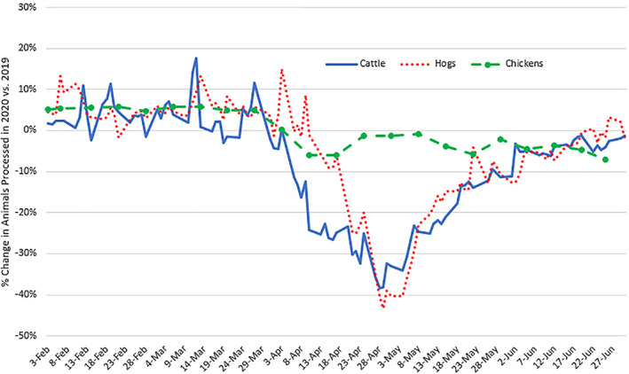
Percent Change in Daily Number of Cattle and Hogs Slaughtered on Weekdays and Weekly Number of Young Chickens Slaughtered in 2020 vs. 2019 [Color figure can be viewed at wileyonlinelibrary.com]
Throughout February and March 2020, cattle, hog, and chicken slaughter were averaging about 5% greater than the same time period in 2019. This reflected both large livestock supplies entering 2020 and industry efforts to pull slaughter forward into the first quarter. However, beginning in April 2020, the effects of COVID‐19 on beef‐ and pork‐packing plants began to appear. Given shutdowns in the rest of the economy, many packing plant workers began staying home, slowing processing volumes. Then, testing revealed workers in a number of packing plants were infected with COVID‐19, leading to a succession of temporary plant shutdowns and further reductions in operating capacity of plants that remained opened.
The worst of the troubles occurred in the last week of April and first of May 2020, when daily processing volumes for beef and pork were both about 40% below the prior year's volumes. Looking at the weekly data (including weekends and holidays), the low point was the week ending May 2, 2020, when beef and pork processing were both 35% below the same week in 2019. The slightly higher slaughter levels reflected in the weekly reports primarily came from extra Saturday operations, especially for hogs.
For the eight weeks following April 5, federally inspected (FI) cattle slaughter averaged 22% lower than the same period in 2019, a decrease of over 1.14 million head, which is nearly two weeks of typical cattle slaughter for that time of the year. For hogs, the reduction was 13% or 2.36 million head, about a week's worth of typical slaughter. These backlogs created significant strain on the livestock supply chains.
Looking at the different classes of livestock and regional slaughter volumes reveals significant differences in the relative impacts of the COVID‐19 pandemic. Not all plants and animal classes were similarly affected. Of most concern was steer and heifer slaughter capabilities as opposed to total cattle slaughter, which also includes dairy cows, beef cows, and bulls.4 Steer and heifer slaughter averaged 79% of total FI cattle slaughter in 2019. Barrow and gilt slaughter accounted for 97% of FI hog slaughter in 2019 with the remainder including sows and boars. For the week ending May 2, FI steer and heifer volumes were 41% lower compared to the same week in 2019 while barrow and gilt volumes were 36% lower.
Much discussion centered on national aggregate FI slaughter volumes, plant‐specific closures, reopenings, and slowdown announcements. State and regional impacts were equally important. The U.S. Federally Inspected Slaughter by Region report (SJ_LS713), also lagged two weeks, shows a breakout of all classes of slaughtered cattle and hogs by region. In 2019, 52% of steer and heifer slaughter occurred in Region 7, including the states of Iowa, Kansas, Missouri, and Nebraska. For the week ending May 2, Region 7 FI steer and heifer slaughter was 48% below the levels of a year earlier. The following week, Region 7 slaughter was down 44% while nationally the year‐over‐year reduction was 34%.
On April 28, 2020, President Donald Trump signed an executive order invoking the Defense Production Act, classifying meat and poultry processors as essential infrastructure in order to help ensure continued operations (Trump 2020). Packers, working with the USDA, state and local public health officials, labor unions, and under guidance from the Centers for Disease Control (CDC) and the Occupational Safety and Health Administration (OSHA) instituted several pandemic‐induced measures, including temperature testing workers, distancing workers inside plants, and installing partitions between workers. By the first week of June 2020, slaughter volumes had recovered and were running about 5% below 2019 production levels for cattle and slightly above 2019 levels for hogs. Still, in aggregate, beef and pork processing was functioning below maximum physical capacity as operational capacity continued to be constrained partly because of the engineered controls and reduced labor availability. By the end of June, cattle slaughter had recovered to 2019 levels and hog slaughter was running above the prior year's levels.
For sake of comparison, figure 1 also reports the year‐over‐year change in the weekly number of young broiler chickens slaughtered. Unlike cattle and hog processing, chicken processing was relatively unscathed by COVID‐19. From February through the end of June 2020, weekly broiler processing was never more than 6% higher or 7% lower than during the same time period in 2019. It is unclear exactly why chicken processing was less affected than beef and pork, but possible explanations include greater use of automation, lower worker density, and differing geographic plant locations. For more on impacts of COVID‐19 on the broiler industry see Maples et al. (2021).
Beef and Pork Wholesale & Livestock Price Patterns
Figure 2 shows weekly Choice boxed beef price from January to the end of June 2020 alongside the negotiated 5‐Area weighted average live FOB steer price (over 80% Choice) as reported by USDA‐AMS and complied by LMIC. The weekly Choice boxed beef price is calculated by the LMIC from the USDA Market News report (LM_XB403), National Daily Boxed Beef Cutout and Boxed Beef Cuts – Negotiated Sales – Afternoon. These values are for negotiated or cash sales, with delivery within twenty‐one calendar days and within the domestic market.5 The 5‐Area Weekly Weighted Average Direct Slaughter Cattle report (LM_CT150) includes cash or spot market purchases where the price is determined through buyer–seller interaction. For negotiated sales, the price is agreed upon at the time the deal is struck and delivery may be up to thirty days. These cutout and steer price series are the ones commonly reported in the media and appear in legal complaints.
Figure 2.
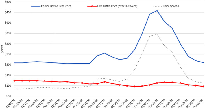
Weekly Wholesale Boxed Beef Value, Live Cattle Price, and Price Spread [Color figure can be viewed at wileyonlinelibrary.com]
Prior to March 2020, wholesale prices were fairly flat, averaging just above $210/cwt. Live steer prices were trending slightly downward over this period, going from about $124/cwt at the first of the year down to $108/cwt by mid‐March. The initial impact of COVID‐19, resulting from reduced food service activity and the spike in demand at groceries, is apparent in the wholesale price data which jumped to $255/cwt at the end of March before falling back down as grocery demand subsided after the initial dramatic adjustment in consumer purchases. Mirroring the reduction in slaughter volumes shown in figure 1, wholesale beef prices increased markedly (figure 2), reaching an apex of $459/cwt for the week ending May 15, 2020. This peak is the highest reported wholesale Choice boxed beef price (in nominal terms) on record.
The price spread, calculated in this case as the difference between the wholesale boxed beef and live steer prices rose in tandem with the wholesale price rise, increasing from an average of about $89/cwt in January and February to a high of $347/cwt in mid‐May, a 292% increase. Figure 2 shows that the rise in the price spread is explained primarily by the rise in wholesale beef prices not by a fall in cattle prices.6 Over the period shown in figure 2 (January 3–June 27, 2020), the coefficient of variation for cattle prices was 8.3%, whereas the coefficient of variation for wholesale boxed beef prices was 30%, implying much greater volatility in wholesale beef prices than cattle prices. A simple regression of log price spread on log wholesale and farm prices indicates a 1% increase in wholesale price is associated with a 1.66% increase in the price spread, whereas a 1% decrease in cattle prices is only associated with a 1.05% increase in the spread.
Because of the long‐standing controversy surrounding the beef marketing margin, figure 3 shows the inflation‐adjusted price spread plotted over a longer period going back to January 2005. The figure reveals the unprecedented nature of COVID‐19, with the price spread in May 2020 more than double previous highs. It is also evident that the price spread has become increasingly volatile over the past five years, highlighting the need to better understand the determinants of changes.
Figure 3.
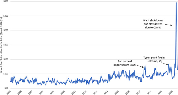
Inflation‐adjusted Weekly Farm to Wholesale Beef Price Spread, January 2005 to June 2020 [Color figure can be viewed at wileyonlinelibrary.com]
Figure 4 shows changes in wholesale pork and dressed hog prices. The overall pattern of price and margin movements in figure 4 for pork is similar to that for beef (figure 2), albeit with less dramatic price movements. The pork margin reflects a farm‐level price measured on a carcass (or dressed) basis (we use the national barrows and gilts weighted average base purchase price across all producer‐sold hogs in the National Daily Direct Hog Prior Day Report–Slaughtered Swine (LM_HG201) by the USDA‐AMS and complied by the LMIC), as relatively few hogs are marketed on a live weight price basis. As was the case for beef, the significant increase in the price spread in May is more explained by the increase in wholesale pork prices than hog prices. The farm‐to‐wholesale pork price spread averaged about $9/cwt in January and February 2020, reaching a peak of almost $44/cwt in early and mid‐May, a 388% increase.
Figure 4.
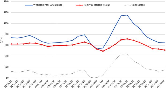
Weekly Wholesale Pork Cutout Value, Dressed Hog Price, and Price Spread [Color figure can be viewed at wileyonlinelibrary.com]
The Theory of Marketing Margin Changes
Before addressing a number of key issues in the measurement and interpretation of marketing margins and price spreads, we first present some basic economic insights on the drivers of changes in marketing margins. The theory of marketing margins has been outlined in previous works such as Gardner (1975), Wohlgenant (2001), and Tomek and Kaiser (2014), among others. Given the increase in price spreads shown in figures 2, 3, 4 associated with COVID‐19, we focus attention on how disruptions in meat processing might affect margins.
Graphical Analysis
The fact that wholesale meat prices can increase at the same time livestock prices are falling can seem almost paradoxical, but these divergent price movements have a straightforward economic explanation. When a packing plant temporarily ceases operations, for instance due to fire or worker illnesses, packers' demand for cattle or hogs falls. That is, a plant closure results in an excess supply of livestock relative to the ability of packers to process them. Plant closures cause a reduction in demand for fed cattle and hogs. As a result, livestock prices fall (see also Tonsor and Schulz 2020).
At the same time, a plant closure means fewer cattle and hogs getting turned into burgers and bacon. A plant closure results in less meat on the market. That is, there is a reduction in meat supply. Grocers, restaurants, and exporters are left vying for a smaller temporary supply of meat, which results in meat prices being bid up. The combined effect of rising wholesale meat prices and falling livestock prices results in an increasing price spread.
The economics are demonstrated more formally in Figure 5. Consider a market in equilibrium prior to any significant disruption. Restaurants and grocery stores want meat for their customers, resulting in the downward sloping “Wholesale Meat Demand” curve. Packer's acquire livestock, process them, and supply meat to the wholesale market, and this relationship is given by the upward sloping line labeled “Packer Meat Supply0”. The intersection of these two lines determines the wholesale price of meat,
Figure 5.
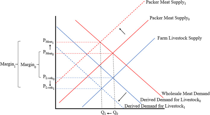
Impacts of a Disruption in the Meat Processing Sector on the Marketing Margin Assuming Fixed Proportions [Color figure can be viewed at wileyonlinelibrary.com]
Because packers need livestock to supply meat to the retail market, they have a derived demand for livestock given by the downward sloping line labeled “Derived Demand for Livestock0.” Livestock producers supply cattle and hogs to the market (as described by the upward sloping blue line marked “Farm Livestock Supply”). The intersection of these two curves determines the price of livestock, at a quantity equal to Q 0 .
To keep matters simple, figure 5 is drawn assuming a model of fixed proportions, meaning every pound of livestock on the farm is equal to a constant fraction of wholesale meat sold (implying the packers cannot substitute labor, packaging, further disassembly, or other marketing inputs for livestock in producing wholesale beef). The difference in the wholesale price of meat, , and the price of livestock,, is the wholesale marketing margin, Margin 0 .
Now, consider an event, such as lost workers and reduced operations from COVID‐19, which hinders the ability of packers to supply meat. This shifts the packer supply curve upward and to the left. As can be seen in figure 5, the result is that wholesale beef prices rise from to .
In addition to packer's supply curve shifting, they cannot utilize as many livestock because they no longer have the capacity to process them. As a result, the derived demand for livestock by the packers also falls. The result is that livestock prices fall from to , and the quantity of meat/livestock sold falls from Q 0 to Q 1 , and the marketing margin increases from Margin 0 to Margin 1 .7
A Simple Model
The determinants of changes in the marketing margin might be seen more clearly using an equilibrium displacement model as outlined by Alston (1991) or Wohlgenant (1993, 2011). We use a straightforward model that makes a number of assumptions such as constant returns to scale, parallel shifts in supply and demand curves, constant elasticities, and perfectly elastic supply of marketing inputs. We also assume away issues like trade and imperfect competition. It might seem strange to assume away the very issue that is at the center of attention (imperfect competition), but the model will show how changes in marketing margins can occur even if there is perfect competition, and we will be able to explore the extent to which observed empirical changes in margins can be explained by a model of marketing margins that assume perfect competition. As reviewed by Wohlgenant (2001), it should be noted that there is a large body of work that has explored the determinants of marketing margins using models similar to that employed here including the seminal work by Gardner (1975). Various extensions to the original model have been proposed that relax the assumption of perfect competition (Holloway 1991) and risk neutrality (Brorsen et al. 1985).
Changes in wholesale meat demand by restaurants and grocery stores are given by
| (1) |
where and are the proportionate changes in the retail quantity and price (e.g., ), respectively, η is the own‐price elasticity of demand, and δ is an exogenous demand shock representing a proportionate increase in retailer/consumer willingness‐to‐pay. The supply of meat and the demand for livestock are given by
| (2) |
| (3) |
where is the proportionate change in the farm‐level quantity of livestock supplied to the packer, is the proportionate changes in livestock price, S is the share of the total cost of producing wholesale meat attributable to livestock, σ is the elasticity of substitution between livestock and marketing inputs in producing meat, and γ is the change in marketing costs. The supply of livestock is
| (4) |
where ε is the own‐price supply elasticity and k is an exogenous supply shifter. Equations (1), (3), (4)) outline a system of equations with four endogenous variables (, , , and ), three exogenous shocks ( δ , γ , and k ), and four parameters ( ε , η , σ , and S ). Solving the system of equations for the farm and retail price yields the following equilibrium values:
| (5) |
| (6) |
There are several ways to define the margin. If the margin is interpreted as a ratio, MR = P/w , as in Gardner (1975), then proportionate changes in this ratio are given by . However, recent legal complaints have focused on the price spread: M = P − w , in which proportionate changes are given by
| (7) |
where the 0 subscript denotes initial equilibrium values (note: and are the inverses of the margin mark‐ups expressed relative to the retail and farm prices, respectively).8 By plugging (5) and (6) into (7), changes in marketing margin are:
| (8) |
Equation (8) clearly shows that changes in marketing margin are a complex mix of shocks to supply, demand, and marketing costs, in addition to magnitudes of elasticities of supply, demand, and substitution. How does an increase in marketing costs influence the margin? Differentiating (8) with respect to γ yields the following:
| (9) |
Given that η < 0, the expression above is positive, and the extent to which the margin changes in response to a change in marketing costs depends on the elasticities of supply and demand as well as the elasticity of substitution between livestock and marketing inputs.9
Margin Definition and Measurement Details
Definitions
Marketing margins can be defined as “… the costs of performing marketing functions required to get live animals from the producer to the consumer” (Ikerd and Ward 1983). This definition is intuitive as it recognizes that cost must be incurred, and reflected in the final product price, in transforming live animals into consumable products. The magnitude of the spread will vary by commodity and even within commodities, depending upon the amount of intermediate processing (Ross 1984). The more processing required, the larger the spread will be. If the intended use of the farm‐to‐wholesale price spread is to demonstrate how marketing costs between farm and wholesale are changing over time, the commonly utilized data is at best a rough indicator which can capture general trends and deviations from trend. The price spread does not provide any direct indication of whether observed price changes are cost‐justified (Mathews et al. 1999). Going further, aggregate marketing margins do not separately measure costs or profits for any one type of firm or industry group. Brester, Marsh, and Atwood (2009) empirically demonstrate that marketing margins are not reliable measures of changes in producer surplus, given exogenous shocks to various economic factors.
Margins for meat packers and livestock producers fluctuate over time, and even within segments, as market leverage ebbs and flows, meaning price spreads between wholesale and farm levels are not precise reflections of marketing costs at any point in time. Over a long‐run horizon, price spreads conceivably reflect marketing costs plus economic profits. However, because of rigidities and lags, at any point in time, the simple spread is not necessarily precise enough for monitoring short‐run or likely even intermediate‐run marketing cost changes.
Occasionally, “gross margin” is mistakenly used for price spread. The two concepts are different. A gross margin is the difference between revenue received and (some) expenses paid by a participant in the marketing system. For example, a packer's gross margin, on a per head slaughtered basis, represents the value of the carcass plus the value of the byproducts less the value of the animal. Data is not readily available on fixed or operating costs (e.g., wages, salaries, administrative expenses, transportation, utilities, insurance, etc.) to calculate a net margin. Even if such data were available, it would be plant and/or firm specific; as such, the net margin would vary within the industry. Because the gross margin only applies for one specific stage in marketing, e.g., meat packing, it does not include costs, beyond the value of the animal, that are included in the price spread. The price spread essentially lumps together costs for several segments, while gross margins apply only to costs for specific segments (Ross 1984). Consequently, we use the term price spread in situations comparing $/cwt data series and marketing margin when making $/head assessments.
Measurement Issues with a Focus on Beef
The preceding section on recent trends in price spreads provides one account of market dynamics that is broadly reflective of the public debate. However, in this section we show that there are a multitude of ways that said margins can be calculated, depending on the intended use of the data.
Estimates of beef margins are provided by USDA‐ERS (2020), LMIC (2020)), and private industry sources (e.g., Sterling Marketing, Inc. 2020). Approaches can vary in terms of which prices are used, if fixed or variable costs are considered, and whether calculations reflect changes in operational throughput. Furthermore, confusion can easily occur given whether calculations are on a $/head and $/cwt basis, if the farm price is based on dressed or live weight sales, and how one calculates the wholesale meat price, given that packers can purchase livestock and convert them into meat products in different ways with resulting different values.
To provide context on how sensitive marketing margin estimates are to methods used, and hence how conclusions regarding economic impacts can be substantially altered, we derive estimates of the marketing margin on a $/head basis considering the following scenarios starting with livestock and wholesale prices and sequentially adding additional considerations.
Packer Gross Margin: No consideration of volumes or costs.
Packer Approximated Net Margin: No consideration of COVID‐19 cost increases.
Packer Approximated Net Margin with COVID‐19 Costs.
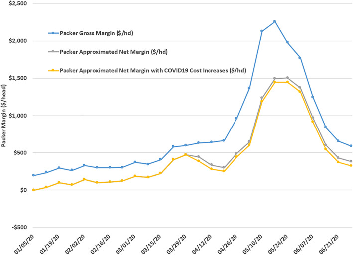
Scenario 1 reflects the process of simply subtracting a livestock purchase price from revenue implied by wholesale meat and drop credit values (see figure 6). Specific variables utilized here include the negotiated weekly weighted‐average, 5‐area total all grades live steer price ($/cwt), and corresponding average weight (pounds) to estimate the total price ($/head) paid for livestock (USDA‐AMS 2020b). To estimate the value of a carcass we use the weekly comprehensive cutout value (USDA‐AMS 2020c) which is the most representative of all wholesale beef transactions.10 We also use steer byproduct drop values (USDA‐AMS 2020d) compiled to a weekly series by LMIC. To derive a $/head margin value, we assume a 2% loss (shrink) from a hot to cold carcass and use each week's average live and dressed weights to obtain hot carcass yields. Combined this results in a Packer Gross Margin estimate which is in $/head units.
Figure 6.
Alternative Calculations of Farm to Wholesale Beef Marketing Margin, January 2004–June 2020 (weighted average 5‐area total all grades fed cattle and comprehensive cutout prices) [Color figure can be viewed at wileyonlinelibrary.com]
In Scenario 2, we proceed from gross margin to net margin values and hence estimates on fixed and variable costs are needed along with operation volume. We use the weekly FI steer and heifer slaughter volume in a current week compared to the same week the prior year to reflect increases and decreases in packing sector operation (USDA‐AMS 2020e). Specifically, we use relative processing volume to identify the share of capacity that actually generates revenue (reflected in the Packer Gross Margin) while the remaining share does not generate revenue.11
Beyond considering volume adjustments, we incorporate operational costs. Cost structures vary widely within the industry and only periodically are estimates made publicly available. However, one analyst remarked: “We think a packer needs to get a little over $200/head to cover processing costs and overhead…” in the June 21, 2018 Daily Livestock Report (DLR 2018). Little guidance exist on how this $200/head estimate is split over fixed and variable costs so we conservatively assume a 50/50 allocation. That is, we presume for the representative situation that $100/head in fixed costs and $100/head in variable costs reasonably represent the pre‐COVID‐19 cost situation for the beef packing sector. This results in a Packer Approximated Net Margin which, by definition, is lower than gross margin estimates. In the week ending May 16, 2020, where Packer Gross Margin peaked, accounting for volumes, fixed costs, and variable costs results in a Packer Approximated Net Margin that is $762/head lower ($2,256 vs. $1,494). The fact this difference in margins exceeds the sum of fixed and variables costs may initially be surprising but is important as it reflects the critical impact of operation volume on revenue generation as well.
Finally, in Scenario 3 we go further and attempt to incorporate a cost inflation reflecting COVID‐19 induced adjustments for the packing sector. Specifically, we presume a $20/head increase in fixed costs and $40/head increase in variable costs applies beginning the week ending April 5, 2020. We admittedly have little guidance on these estimates and include them to reflect the widely recognized efforts to increase provision of PPE, increase labor wages, etc. In the week ending May 16, accounting for volumes, fixed costs, variable costs, and COVID‐19‐induced costs results in a Packer Approximated Net Margin with COVID‐19 Costs, which is $811/head lower ($2,256 vs. $1,445).
To further highlight how the approach taken has a significant impact on conclusions consider the results in table 1. Here margin estimates for the week ending May 16th are presented for the actual processing rate of 74% as well as alternatives of 60% and 90% of prior year volumes.
Table 1.
Beef Marketing Margins by Processing Rate Implied for Week Ending May 16, 2020
| Processing rate (% of prior year) | Packer gross margin ($/hd) | Packer approximated net margin ($/hd) | Packer approximated net margin with COVID‐19 cost increases ($/hd) |
|---|---|---|---|
| 73.94% | $2,256 | $1,494 | $1,445 |
| 60% | $2,256 | $1,194 | $1,150 |
| 90% | $2,256 | $1,841 | $1,785 |
Key points include noting that ignoring costs and volume aspects results in the erroneous conclusions that marketing margins are the same regardless of the processing rate accomplished by a facility. Accounting for both fixed and variable costs obviously results in lower margin conclusions, but of central importance is the observation that plants are incentivized to operate at higher processing rates. Examining the difference in margins when facilities operate at 90% of capacity versus 60% clearly demonstrates this key point. While specific margin estimates are functions of wholesale meat prices, livestock prices, and costs these qualitative differences hold across price and cost levels.
To better assess COVID‐19 impacts and the industry's well‐debated “bottleneck” challenge, it is useful to back up and consider what might have been expected given past relationships of packer margins with livestock prices, boxed beef prices, and slaughter volumes. Here we use the Packer Gross Margin and Packer Approximated Net Margin estimates discussed above for the January 2004–December 2018 period to facilitate further assessment. We start with data in 2004 given changes in wholesale meat price information and stop in 2018 to avoid related complications with the August 2019 Holcomb, Kansas packing plant fire event. Simple regressions of these two alternative margin series are summarized in table 2.
Table 2.
Relationship between Alternative Beef Marketing Margin Estimates, Prices, and Slaughter Volume
| Variable | Packer gross margin ($/hd) | Packer approximated net margin ($/hd) |
|---|---|---|
| Intercept | 45.096 | −271.377 |
| Wtd Avg Fed Cattle Price ($/cwt) | −11.065 | −11.093 |
| Comp. Cutout Value ($/cwt) | 7.599 | 7.654 |
| FI Slaughter (Steers & Heifers) as % of Last Year | – | 111.391 |
| Adjusted R Square | 0.882 | 0.885 |
| Observations | 783 | 783 |
Note: All presented coefficients are statistically significant at the 1% level.
In the first model, Packer Gross Margin is regressed against fed cattle and cutout prices without any control for volume changes consistent with how the Packer Gross Margin is often reported. The positive intercept estimate would suggest that if cattle and wholesale beef prices were $0, packers would have a positive gross margin of $45/head. This is inconceivable and reinforces the importance of controlling for production volumes in any margin assessment.
When alternatively, the Packer Approximated Net Margin series is regressed against prices and volume changes, a more reasonable set of results is obtained. The negative intercept estimate of $271 indicates that if volume did not change from the prior year and both cattle and beef prices were $0, margins would be negative—a much more viable conclusion. Consistent with expectations, margins decline as cattle procurement prices increase and margins increase as boxed beef prices escalate, all else equal. The positive coefficient on volume changes indicates that for each 1% increase (decrease) in throughput, compared to the prior year, gross margins increase (decrease) by $1.11/head.
Across these regressions two additional key points are revealed. First, the ratio of cattle and boxed beef price coefficients is remarkably close to the biologically driven dressing percentage. Specifically, the comprehensive cutout price coefficient is 69% the magnitude of the weighted average fed cattle price (in absolute terms). Meanwhile, for the 2004–2018 period the implied dressing percentage in USDA's 5‐Area Weekly Weighted Average Direct Slaughter cattle (LM_CT150) report averaged 65.2%. The very similar relationships revealed by these regressions is noteworthy. There is nothing in a simple regression that forces this relative price impact estimate, rather this reflects the inner workings of cattle‐buying and wholesale beef‐selling markets that are revealed here to be strongly in line with base biology of dressing yield percentage (which varies over time).12 On balance, the more competitive markets are in an industry, the more economists would anticipate similar findings. Conversely, if there was undue market power or forces at play in either the fed cattle or wholesale beef market it seems very unlikely this regression finding would persist.
Secondly, these regressions can be used to directly speak to the 2020 situation.13 For the week ending May 2, the sector operated at 59% of the prior year's steer and heifer slaughter volume. Between March 1 and May 2, fed cattle prices declined about $16/cwt and boxed beef prices increased about $96/cwt. Using these three changes and the estimates in the last column in table 2 leads to a predicted increase of $957/head in the marketing margin―of which, 77% ($734) is tied to higher wholesale meat prices. Meanwhile, our calculations for what occurred indicate the Packer Approximated Net Margin increased by $460/head. The key point is yes, the marketing margin widened notably but this was predictable and consistent with economic theory. The fact that the actual margin change was about 50% less than the $957/head projected by the Packer Approximated Net Margin model in table 2, using pre‐COVID‐19 data is noteworthy.
As a final example to document the sensitivity of margin estimates to procedures employed, consider the impact of changing presumed fed cattle prices. In 2017, USDA began publishing the National Weekly Fed Cattle Comprehensive (LM_CT200) report which combines negotiated formula net, forward contract net, and negotiated grid net purchase information into a single weekly price series. As such, this report reflects a larger volume of fed cattle transactions and arguably provides a more representative estimate of what packers pay (and producers receive) for fed cattle than the negotiated 5‐Area (total all grade, weighted average) price used in our margin assessments. In fact, in the first six months of 2020, a total of 1.04 million head were reported in the 5‐Area (LM_CT150) series while over 9.3 million head were reported in the comprehensive (LM_CT200) series (total of live and dressed volumes). As shown in figure 7, for the entire April–June period in 2020 the Packer Approximated Net Margin series is much lower when the comprehensive (LM_CT200) price is used. This difference was largest, averaging 31% lower, in April.
Figure 7.
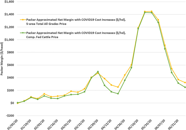
Impact of Fed Cattle Price Selection on Farm to Wholesale Beef Marketing Margin Calculations, January 2004–June 2020 [Color figure can be viewed at wileyonlinelibrary.com]
While not directly incorporated into the calculations here, it should be noted that amid COVID‐19 disruptions, some packing plants made changes to fabrication, leaving more whole muscles/primals intact and keeping less offal in order to maximize line speed as much as possible. This impacts both the revenue side and costs sides of the marketing margin equation. Furthermore, the exact magnitude of COVID‐19 based cost increases and the proportion that are fixed in nature will notably influence margins going forward. Accordingly, additional research documenting these adjustments is encouraged.
Discussion
It is not surprising that during a human pandemic, casting wide impacts throughout society, seemingly paradoxical observations of livestock prices declining while wholesale meat prices are increasing would garner widespread scrutiny. Given harm to producers and consumers caused by the adverse price movements and the economic importance of industries and stakeholders involved, this study attempts to add clarity and nuance to the discussion. The overriding goal of this paper was to provide data‐driven and economic‐guided insights to document the situation and improve related dialogue. This study provides price spread and marketing margin details for the U.S. beef cattle and pork swine industries, documents how economist expectations on directional impacts have been affirmed using multiple approaches, and demonstrates important impacts that data and calculations have on final conclusions.
Operating a packing plant at lower capacity with workers spaced out for social distancing is costly. It is also costly to close down, refrigerate empty buildings, pay employees who aren't at work, pay overtime, install partitions between workers, deal with legal challenges, etc. We document the impact of these costs and encourage additional work to more precisely quantify these impacts if, and when, additional data becomes available. Presumably, if it was in a packer's interest to significantly reduce capacity, they could have closed down any of their plants prior to the emergence of COVID‐19. The fact that they did not voluntarily shut down processing facilities suggests they believe they are better off trying to run near capacity―a fact affirmed by our work here. Beyond the immediate economic incentives, there were also broader societal considerations related to keeping plants operational related to issues surrounding worker safety but also food availability for consumers.
All that said, it is of course, possible that packers were more profitable during COVID‐19‐related disruptions. Unexpected, exogenous shocks will cause changes in the economic well‐being of packers, livestock producers, and consumers, even if none are directly responsible for the changes. Even though we cannot observe an individual packers' costs, we can observe the market's perception of their profitability―at least for publicly traded firms.14 On balance, changes in the stock prices of companies with significant packing operations do not suggest substantial windfalls corresponding with COVID‐19 driven developments, and indeed the performance of publicly traded packing companies has lagged that of the overall market since the first of the year. Perhaps market developments are rationale responses to massive shocks from a common enemy to society, COVID‐19. Nonetheless, issues related to competitive behavior in the meat‐packing sector have been contentious for some time (Wohlgenant 2013).
Because price spreads and margins are often discussed in the context of concentration and potential anticompetitive behavior, it is useful to review changes (or lack thereof) in scale concentration over time. Here we draw on data for FI plants and head slaughtered by size group for cattle provided in USDA National Agricultural Statistics Service (USDA‐NASS, 2020b) Livestock Slaughter Annual Summary reports. In 1998, FI packing plants that slaughtered more than one million cattle per year slaughtered 17.9 million head, or 51.7%, of the FI cattle slaughter. More than 20 years later, in 2019, plants with over one million head per year capacity slaughtered 17.3 million head, or 52.4%, of the FI slaughter. The total volume slaughtered by the largest plants is down, and it is a stretch to characterize a 0.7% rise in slaughter market share over 22 years as a takeover. This suggests that smaller FI slaughter facilities, in aggregate, are maintaining market share. In 2019, packing plants that slaughtered between one and 9,999 head collectively slaughtered 424,700 head, or 1.3%, of the FI cattle slaughter annually, 3.3% for plants slaughtering between 10,000 and 99,999 head, and 43.1% for plants slaughtering between 100,000 and 999,999 head. This compares to 1.5%, 4.7% and 42.1%, respectively, in 1998.
The US has fewer FI cattle slaughter plants than it had 20 years ago. But the current number of FI plants is the highest since 2004. In 1998, the US had 795 FI cattle slaughter plants. Plant numbers bottomed at 626 in 2007 and 627 in 2012, before reaching 670 in 2019. In 2019, 71.6% of FI slaughter plants each slaughtered between 1 and 999 head annually, 16.0% slaughtered between 1,000 and 9,999 head, and 10.6% slaughtered between 10,000 and 999,999. This compares to 71.7%, 14.8% and 11.7%, respectively, in 1998. Plants that each slaughtered over one million head only comprised 1.8% of the total number of US. FI cattle slaughter facilities in both 1998 and 2019. Nonetheless, it remains the case that roughly 60% of total beef‐and pork‐processing capacity is provided by the 10 largest beef‐ and the 15 largest pork‐packing plants (National Pork Board 2019).
Economies of scale are an important component of meat processing. The ability to spread costs (such as labor, overhead, transportation, etc.) over a larger throughput allows larger facilities to produce higher volumes at lower costs per animal than smaller facilities can (e.g., MacDonald and Ollinger 2000, 2005). However, with the COVID‐19‐related disruptions in meat packing and the resulting backlog of animals, the sheer abilities of scale is an important consideration. Efforts to find alternative outlets outside the conventional or typical processing channels for market‐ready animals were fruitful when FI slaughter capacity was severely impacted. However, an upper bound exists on state‐inspected, custom‐exempt, and on‐farm slaughter as these facilities face many constraints such as physical infrastructure, equipment, cooler space, and availability of skilled labor.
Consumers desire meat products, packers need producers to raise livestock, and producers need packers to convert livestock into end‐user goods. Changes in industry structure, the nature of price discovery and public reporting, and economic signals to align production effort with consumer demand have long been core to the viability of the US meat‐livestock industry. The modern realities of a pandemic response include multiple calls for government intervention and industry adjustment. The concepts of derived demand and supply for livestock and wholesale meat, as well as long‐term implications of possibly adding costs to a sector that has evolved around efficiencies and economies of scale central to prepandemic operation must be considered. There is a tradeoff between a system that provides efficiency and affordable meat for consumers in “normal times” and the costs associated with adding capacity, flexibility, and resiliency to a sector for “abnormal” times. We concur with USDA‐AMS (2020) in their assessment of related industry developments: “it is important that any proposals aimed at addressing these complex issues and others associated with the disruptions caused by the Holcomb fire and COVID‐19 receive careful consideration and thorough vetting given their potential to affect everyone whose livelihood depends on the sales of cattle, beef, or related products.” Hopefully this study serves as a launching point in related assessments.
Jayson L. Lusk is a distinguished professor and head of the Department of Agricultural Economics at Purdue University. Glynn T. Tonsor is a professor at the Department of Agricultural Economics at Kansas State University. Lee L. Schulz is an associate professor at the Department of Economics at Iowa State University.
Editor in Charge: Craig Gundersen.
Footnotes
In this paper, we focus on the farm‐to‐wholesale margin because publicly reported farm and wholesale price data are released in a timely and operational manner. At the retail level, the complexity dramatically increases because of the number of different products involved and alternative market outlets (e.g., grocery store, food service, online shopping, and export) along will the lag in data being released. Furthermore, much of the litigation has focused on the packing sector.
There is an important distinction between price spreads and marketing margins, which we discuss later in the paper.
There are approximately 800 livestock slaughter plants in the United States operating under Federal Inspection (FI) and about 1,900 Non‐Federally Inspected (NFI), either state‐inspected or custom‐exempt, slaughter plants (USDA NASS 2020). This includes slaughter of cattle, calves, sheep, lambs, and hogs. Slaughter from state‐inspected Talmadge‐Aiken plants (where the USDA has contracted with state agency inspectors to carry out federal inspection) is included in FI totals. FI slaughter accounts for the majority of volume. Total commercial US cattle slaughter in 2019 was 33.555 million head, of which 33.069 million head, or 98.6%, was FI. Similarly, total commercial US hog slaughter in 2019 was 129.913 million head, of which 129.211 million head, or 99.5%, was FI.
Steers and heifers are the primary output of the US beef supply chain. Slaughter cows and bulls are residual outputs of dairy enterprises and beef‐breeding herds. The beef cattle industry has some flexibility to adjust cattle flows and timing at the calf and feeder cattle and cull cow and bull stages of production. The production and marketing windows for finished cattle are much narrower, as finished fed cattle are not readily storable. Bottlenecks and backlogs in the pork supply chain, with barrows and gilts being the primary output, are especially acute given the shorter biological lags.
There are some important caveats to mention with respect to the wholesale meat prices discussed here. Wholesale meat prices are summarized by a USDA reported carcass equivalent or “cutout” basis. A carcass equivalent is not a price per se, but a value derived from individual meat cut prices put on a carcass equivalent basis. So, it is a rather broad measure and has many assumptions. A set of yields are used to aggregate individual cuts into primal components (rib, chuck, round, loin, brisket, short plate, and flank for beef). Then another set of yield proportions are applied to primals to derive the aggregate cutout, which is a carcass equivalent value. Note that the yields are fixed for a period of time by USDA and updated periodically using industry input. Changes in the reported cutout values are due to the underlying prices for cuts which are weighted by quantity sold. This weighted average causes items sold in largest quantity to have the most effect on the cutout. Further details regarding USDA boxed beef reports are available at https://www.ams.usda.gov/sites/default/files/media/USDADailyBoxedBeefReport.pdf.
A similar phenomenon was observed after the Holcomb, Kansas packing plant fire in August 2019.
It is possible to use an unexpected reduction in packer supply (e.g., a plant closure from a random fire) to estimate the elasticity of wholesale demand for meat and the derived demand for livestock. As figure 5 shows, neither of these curves shifted, thus any price changes occur because of movements along these curves, which enables one to estimate of the slope of the curve. Following the Tyson plant fire in August 2019, about 6% of national processing capacity was lost (i.e., quantity of meat supplied fell by 6%) and boxed beef prices increased by about 13%, yielding an estimate of the elasticity of demand for wholesale beef of −6%/13% = −0.46, which is very similar to the wholesale demand for Choice beef estimated by Lusk et al. (2001) of −0.43 using a conventional econometric approach.
Although the expression for is simpler than that for , we focus on the latter because the two are not always the same sign, and the latter has been given more attention in legal complaints. Attention has focused on the difference in wholesale and farm prices, and as such, we focus on that difference here. However, as pointed out by Wohlgenant (2001), the margin should be defined as: because the farm price needs to be expressed in retail equivalent units. Under the assumption of fixed proportions, σ = 0, Q = x , and M = P − w .
It would be possible to empirically implement the model using elasticity estimates for a livestock industry to infer the size of the marking cost increase, γ , that would be needed to generate the increase in price spreads observed in figures 2 and 4. However, the model expresses equilibrium outcome predictions, which are longer‐run effects after supply responds, packers exercise ability to substitute nonanimal inputs for livestock, whereas the figures show immediate price impacts, where the market has not yet achieved an equilibrium.
Includes all sales types, all delivery periods, and all delivery locations. An overview of the comprehensive boxed beef cutout report is available at https://www.ams.usda.gov/sites/default/files/media/Comprehensive%20Boxed%20Beef%20Cutout%20Overview%20PDF.pdf.
The Packer Approximated Net Margin is calculated as: (Packer Gross Margin – Variable Cost)*(FI Slaughter this Week / FI Slaughter Last Year Same Week) – Fixed Costs.
Derivation of carcass revenue incorporates dressing yields implied by live and dressed cattle transactions and average weights while derivation of cattle procurement costs reflects average weights. That is, there is nothing in the calculation of margins here that “forces” regression results to align with biological yield relationships.
Unique aspects of COVID‐19 should make analysts cautious in heavily relying on pre‐COVID based‐models. However, use of pre‐COVID‐19 models provides a data‐driven framework not feasible from use of qualitative or merely observational approaches.
The price of a stock reflects the market's expectations of a firm's profitability, and one widely accepted model of stock price determination is that stock prices reflect the net‐present value of all future dividends (i.e., profits) paid to shareholders.
References
- Alston, Julian M. 1991. Research Benefits in a Multimarket Setting: A Review. Review of Marketing and Agricultural Economics 59: 23–52. [Google Scholar]
- Brester, Gary W. , Marsh John M., and Atwood Joseph A.. 2009. Evaluating the Farmer's‐Share‐of‐the‐Retail‐ Dollar Statistic. Journal of Agricultural and Resource Economics 34: 213–236. [Google Scholar]
- Brorsen, Wade B. , Chavas Jean‐Paul, Grant Warren R., and Schnake L.D.. 1985. Marketing Margins and Price Uncertainty: The Case of the US Wheat Market. American Journal of Agricultural Economics 67(3): 521–528. [Google Scholar]
- Bunge, Jacob , and Kendall Brent. 2020. Justice Department Issues Subpoenas to Beef‐Processing Giants. Wall Street Journal. June 5, 2020, https://www.wsj.com/articles/justice-department-issues-subpoenas-to-beef-processing-giants-11591371745
- Daily Livestock Report . 2018. June 22, 2018 issue. http://www.dailylivestockreport.com/documents/dlr%2006-22-18.pdf
- Gardner, Bruce L. 1975. The Farm‐Retail Price Spread in a Competitive Food Industry. American Journal of Agricultural Economics 57(3): 399–409. [Google Scholar]
- Holloway, Garth J. 1991. The Farm‐Retail Price Spread in an Imperfectly Competitive Food Industry. American Journal of Agricultural Economics 73(4): 979–989. [Google Scholar]
- Ikerd, John E. , and Ward Clement E.. 1983. Price Spreads: Cattlemen's Share and Effects on Cattle Prices. Stillwater, OK: Oklahoma State University Extension Facts, No. 470.
- Livestock Marketing Information Center (LMIC) . 2020. https://lmic.info/content/about-lmic
- Lusk, Jayson L. , Marsh Thomas L., Schroeder Ted C., and Fox John A.. 2001. Wholesale Demand for USDA Quality Graded Boxed Beef and Effects of Seasonality. Journal of Agricultural and Resource Economics 26: 91–106. [Google Scholar]
- MacDonald, James M. , and Ollinger Michael E.. 2000. Scale Economies and Consolidation in Hog Slaughter. American Journal of Agricultural Economics 82(2): 334–346. [Google Scholar]
- MacDonald, James M. , and Ollinger Michael E.. 2005. Technology, Labor Wars, and Producer Dynamics: Explaining Consolidation in Beefpacking. American Journal of Agricultural Economics 87: 1020–1033. [Google Scholar]
- Maples, Joshua G. , Thompson Jada M., Anderson John D., and Anderson David P.. 2021. Estimating Covid‐19 Impacts on the Broiler Industry. Applied Economic Perspectives and Policy 43(1): 315–328. 10.1002/aepp.13089. [DOI] [Google Scholar]
- Martinez, Charles C. , Maples Joshua G., and Benavidez Justin. 2021. Beef Cattle Markets and COVID‐19. Applied Economic Perspectives and Policy 43(1): 304–314. [Google Scholar]
- Mathews, Kenneth H. , Hahn William F., Nelson Kenneth E., Duewer Lawrence A., and Gustafson Ronald A.. 1999. U.S. Beef Industry: Cattle Cycles, Price Spreads, and Packer Concentration. Washington DC: U.S. Department of Agriculture, Technical Bulletin 1874.
- National Pork Board . 2019. Estimated Daily U.S. Slaughter Capacity by Plant. September 30, 2019. https://www.pork.org/facts/stats/u-s-packing-sector/
- Ross, JohnW . 1984. Farm‐to‐Retail Price Spreads for Livestock. Reciprocal Meat Conference Proceedings 37, 129–133. https://www.meatscience.org/docs/default-source/publications-resources/rmc/1984/farm-to-retail-price-spreads-for-livestock.pdf?sfvrsn=ac1fbbb3_2
- Sterling Marketing, Inc ., 2020. Sterling Beef Profit Tracker. https://cdn.farmjournal.com/s3fs-public/inline-files/Beef%20Tracker%2041520.pdf
- Tomek, William G. , and Kaiser Harry M.. 2014. Agricultural Product Prices. Ithaca, NY: Cornell University Press. [Google Scholar]
- Tonsor, Glynn and Schulz Lee. 2020. Assessing Impact of Packing Plant Utilization on Livestock Prices. Kansas State University, Department of Agricultural Economics, KSU‐AgEcon‐GTT‐2020.2, April 4. https://www.agmanager.info/livestock-meat/marketing-extension-bulletins/price-risk/assessing-impact-packing-plant-utilization
- Trump, Donald J . 2020. Executive Order on Delegating Authority Under the DPA with Respect to Food Supply Chain Resources During the National Emergency Caused by the Outbreak of COVID‐19. U.S. White House. April 28. Available online at: https://www.whitehouse.gov/presidential-actions/executive-order-delegating-authority-dpa-respect-food-supply-chain-resources-national-emergency-caused-outbreak-covid-19/
- USDA Agricultural Marketing Service (USDA‐AMS) . 2020. Boxed Beef & Fed Cattle Price Spread Investigation Report. July 22, 2020. https://www.ams.usda.gov/sites/default/files/media/CattleandBeefPriceMarginReport.pdf
- USDA‐AMS . 2020b. 5‐Area Weekly Weighted Average Direct Slaughter Cattle. https://www.ams.usda.gov/mnreports/ams_2477.pdf
- USDA‐AMS . 2020c. National Comprehensive Boxed Beef Cutout – All Fed Steer/Heifer Sales. https://www.ams.usda.gov/mnreports/lm_xb463.txt
- USDA‐AMS . 2020d. USDA By‐Product Drop Value (Steer) FOB Central U.S. https://www.ams.usda.gov/mnreports/nw_ls441.txt
- USDA‐AMS . 2020e. Actual Slaughter Under Federal Inspection. https://www.ams.usda.gov/mnreports/sj_ls711.txt
- USDA‐ERS . 2020. Meat Price Spreads. https://www.ers.usda.gov/data-products/meat-price-spreads/
- USDA National Agricultural Statistics Service (USDA‐NASS) . 2020. Livestock Slaughter 2019 Summary. April 22. https://downloads.usda.library.cornell.edu/usda-esmis/files/r207tp32d/34850245n/5712mr72x/lsan0420.pdf
- USDA‐NASS . n.d. Livestock Slaughter; Various Reports. 2020b. https://usda.library.cornell.edu/concern/publications/rx913p88g
- Wohlgenant, Michael K. 1993. Distribution of Gains from Research and Promotion in Multi‐Stage Production Systems: The Case of the US Beef and Pork Industries. American Journal of Agricultural Economics 75: 642–651. [Google Scholar]
- Wohlgenant, Michael K. 2001. Marketing margins: Empirical analysis. In Handbook of Agricultural Economics, Vol 1, ed. Gardner Bruce L. and Rausser Gordon C., 933–970. Amsterdam: Elsevier. [Google Scholar]
- Wohlgenant, Michael K. 2011. Consumer demand and welfare in equilibrium displacement models. In Oxford Handbook of The Economics of Food Consumption and Policy, ed. Lusk Jayson L., Roosen Jutta, and Shogren Jason F., 292–319. Oxford, UK: Oxford University Press. [Google Scholar]
- Wohlgenant, Michael K. 2013. Competition in the US Meatpacking Industry. Annual Review of Resource Economics 5: 1–12. [Google Scholar]