Faraday waves in soft elastic solids

Abstract

Recent experiments have observed the emergence of standing waves at the free surface of elastic bodies attached to a rigid oscillating substrate and subjected to critical values of forcing frequency and amplitude. This phenomenon, known as Faraday instability, is now well understood for viscous fluids but surprisingly eluded any theoretical explanation for soft solids. Here, we characterize Faraday waves in soft incompressible slabs using the Floquet theory to study the onset of harmonic and subharmonic resonance eigenmodes. We consider a ground state corresponding to a finite homogeneous deformation of the elastic slab. We transform the incremental boundary value problem into an algebraic eigenvalue problem characterized by the three dimensionless parameters, that characterize the interplay of gravity, capillary and elastic waves. Remarkably, we found that Faraday instability in soft solids is characterized by a harmonic resonance in the physical range of the material parameters. This seminal result is in contrast to the subharmonic resonance that is known to characterize viscous fluids, and opens the path for using Faraday waves for a precise and robust experimental method that is able to distinguish solid-like from fluid-like responses of soft matter at different scales.

1. Introduction

In 1831, Faraday first observed standing capillary waves at the free surface of several fluids on a thin plate subjected to a periodic vertical oscillation [1]. Notably, he remarked that the characteristic frequency of the emerging patterns was half that of the driving frequency of the imposed vibration. This seminal observation of subharmonic resonance later inspired Lord Rayleigh in 1883 to propose a theoretical explanation based on a parametric oscillator governed by the Mathieu equation [2]. The analytic solution of the linear stability analysis for an ideal fluid was given after several decades by Benjamin and Ursell, showing a marginal stability diagram alternating loci of subharmonic and harmonic (i.e. isochronous) resonance [3].

The later analysis for a viscous fluid has shown that the dominance of a resonance mode over the other is mainly controlled by the ratio between the basin height and the typical length-scale of the viscous boundary at the free surface [4,5]. Subharmonic resonance dominates in the nearly inviscid case, while bicritical points where both modes emerge simultaneously are encountered in shallow basins since the viscous effects are enhanced by the presence of the bottom rigid substrate [6]. The emergence of Faraday waves having a critical wavenumber is observed when the acceleration of the vertical oscillation reaches a critical threshold. Cubic terms are the weakest nonlinearities allowed to resonate with subharmonic linear eigenmodes in the associated amplitude equations, thus controlling the morphological transition to a large variety of ordered patterns [7]. Similar to other supercritical fluid instabilities [8], in the subharmonic regime, the selection and the weakly nonlinear development of such patterns is mainly driven by the shape of the edge constraints of the basin [9,10]. In the case where subharmonic and harmonic eigenmodes compete near the instability threshold, the patterns can arrange to a superlattice, localize in space and display chaotic motion on a slow timescale [11]. In experimental conditions with flexible boundaries, Faraday waves enable a localized wave particle interaction reminiscent of quantum mechanics, resulting into complex dynamics of self-propagation [12,13].

In this work, we aim to characterize the interaction of elastic, gravity and capillary waves for the onset of Faraday instability in soft solids. The elastic behaviour of the medium has been recently found to have a dramatic regularizing effect on some well-known dynamic phenomena in fluid mechanics, such as Rayleigh-Plateau [14,15] or Rayleigh-Taylor instabilities [16–18]. Despite the recent experimental interest in this subject, very little is known about the elastic effects on the propagation of Faraday waves. For non-Newtonian solutions of polymers, it has been observed that the instability threshold increases with respect to the Newtonian case as the driving frequency increases, suggesting that viscosity of the solution conversely decreases [19]. For linear viscoelastic fluids, the resonant mode becomes harmonic in the range where elastic forces are of the same order as the surface tension at the free boundary [20,21]. Moreover, the corresponding instability diagram is strongly affected by variations of the liquid relaxation time [22]. For soft solids, recent experiments reported the dispersion relations of standing waves in soft agarose gels [23], paving the way for a positive use of Faraday instability to measure the rheological properties of complex matter at scales where capillary-gravity and Rayleigh waves interact.

This work is organized as follows. In §2, we show some recent experimental results highlighting the emergence of standing waves in soft slabs subjected to a vertical oscillation. In §3, we define the nonlinear elastic problem and identify its homogeneous solution as the ground state. In §4, we derive the incremental boundary value problem that is solved using the Floquet theory, considering both harmonic and subharmonic resonance modes. In §5a, we define the dimensionless parameters governing the problem and in §5b, we collect both the numerical and the analytical results of the linear stability analysis. Finally, we collect in §5c the results of the marginal stability analysis with respect to the governing dimensionless parameters, adding with few concluding remarks in §6.

2. Experimental investigation of Faraday waves in soft materials

We have observed Faraday waves on agarose gels using the experimental set-up shown in figure 1a. Here, a square plexiglass container with edge length 9 cm is affixed to a mechanical shaker which vertically drives the container over a range of frequencies $f_d=30-90\hspace{0.17em}\text{Hz}$ to give the images presented in figure 1b. The amplified signal of a function generator is used to drive the shaker, and the container acceleration is measured using an accelerometer mounted to the tank support. The soft materials used in these experiments are agarose gels made by dissolving agarose powder (Sigma Aldrich Type VI-A) in warm deionized water. The liquid is then allowed to gel in a container having a height h = 24 mm. The rheology of the gels are measured using an Anton Paar MCR-302 rheometer which admits a complex modulus G′ + iG″. The storage modulus is typically many orders of magnitude larger than the loss modulus G′ ≫ G″ implying that these gels behave as an elastic solid with shear modulus in the range μ = 1 − 300 Pa. Because our gels are soft, they are also subject to surface tension effects and the observed properties of the Faraday waves depend upon the resistance to motion caused by both shear modulus μ and surface tension γ with the relative importance quantified by the elastocapillary length ℓ = γ/μ. An advantage of exploring these soft agarose hydrogels is that these materials are often used in cell-printing applications for tissue engineering because they are capable of sustaining biological function. Studying Faraday wave formation in these gels may facilitate methods for patterning cells in a hydrogel matrix.

Figure 1.

Faraday waves in soft gels: (a) schematic of experimental set-up, (b) typical wave pattern for a gel with shear modulus μ = 19 Pa in a square container, as it depends upon driving frequency f, and (c) typical instability tongue plotting critical acceleration a against frequency f for a given mode in a circular container.

Above a critical acceleration threshold, waves appear on the gel surface as shown in figure 1b, which tend to exhibit square-wave symmetry and align with the container geometry. For low driving frequency, the surface wave exhibits a discrete mode number and finite bandwidth over which that mode can be excited [7,9]. The bandwidth is illustrated in the typical instability tongue shown in figure 1c. Here, the resonance frequency ≈11 Hz coincides with the minimum value of the threshold acceleration. In general, for high driving frequency, the instability tongues become clustered closer together, there is no longer a finite bandwidth, the spatial wavenumber k is continuous, and the container geometry does not affect the wave pattern, as shown by [24] using irregular container geometries. The wavenumber k increases with the driving frequency and for accelerations much above threshold the waves lose their symmetry and become chaotic in nature. In our theoretical development, we assume the wavenumber is continuous and this corresponds to the high-frequency limit. We have also measured the critical acceleration for Faraday wave onset using essentially the same set-up shown in figure 1, except using a circular tank. The HeNe laser beam (632.8 nm) shown in the figure is directed at the gel surface, and the reflected beam is captured by a position sensitive detector (PSD). The PSD output gives the location of the centroid of the light striking the detector which, in these experiments, is essentially the location of the laser spot on the detector. The vertically oscillating gel surface results in an oscillating signal from the PSD whose frequency is obtained via an FFT to yield the surface wave frequency f_o. In our experiments, we observe that f_o = 0.5f_d, a subharmonic response which is a signature of Faraday waves. We have obtained Faraday wave tongues by fixing f_d, performing an amplitude sweep and locating the threshold acceleration a_c. By repeating this for a range of f_d, Faraday wave tongues are traced out in a − f_d space. An example of such a tongue is presented in figure 1c for the case of an agarose gel having an elasticity of μ = 3.5 Pa.

3. The nonlinear elastic problem and its ground state

Let ${\mathbb{E}}^3$ be the three-dimensional Euclidean space, we consider a soft hyperelastic body with a reference domain ${\mathrm{\Omega }}_0\in {\mathbb{E}}^3$ in its undeformed state. The body is infinitely long along the Z direction, so that a plane strain assumption can be made, hence

$${\mathrm{\Omega }}_0=\{\mathit{X}=[X,Y,Z]\in {\mathbb{E}}^3:X\in (0,L),Y\in (0,H),Z\in \mathbb{R}\},$$

where H is the reference height, L is the reference length and X is the material position vector. The body is attached to a rigid substrate at Y = 0 and free to slide at the lateral walls X = 0, X = L, being subjected to its own weight and to a vertical sinusoidal oscillation of amplitude a and frequency ω, as sketched in figure 2. We consider in the following a Cartesian coordinate system that is fixed with the rigid substrate, with unit material vectors E_i, with i = X, Y, Z,

Figure 2.

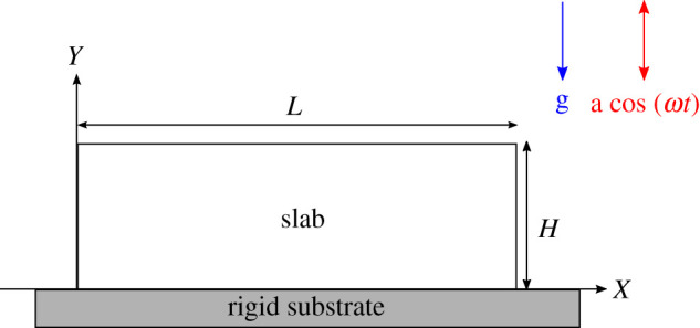
Sketch of the reference configuration of the model: L is the reference length of the elastic slab and H is its reference height. It is clamped to a rigid substrate and it is subjected to its own weight and to a vertical sinusoidal oscillation with amplitude a and frequency ω. (Online version in colour.)

The actual position vector is given by x = χ(X, t), where $\mathit{\chi }:{\mathrm{\Omega }}_0\to \mathrm{\Omega }\in {\mathbb{E}}^3$ is a one-to-one mapping at time t, so that the kinematics of motion is described by the geometrical deformation tensor $\mathsf{F}=\text{Grad}\hspace{0.17em}\mathit{x}=\mathrm{\partial }\mathit{x}/\mathrm{\partial }\mathit{X}$. We also assume that the body is made of an incompressible neo–Hookean material with strain energy density given by

$$W(\mathsf{F})=\frac{\mu }{2}(\text{tr}\hspace{0.17em}\mathsf{C}-2)-p(\text{det}\hspace{0.17em}\mathsf{F}-1),$$ 3.1

where μ is the shear modulus, $\mathsf{C}={\mathsf{F}}^T\mathsf{F}$ is the right Cauchy–Green tensor and p is the Lagrangian multiplier enforcing the internal constraint of incompressibility. Using the constitutive assumption in equation (3.1), the nominal stress tensor $\mathsf{S}$ and the Cauchy stress tensors $\mathsf{T}$ are given, respectively, by [25]

$$\mathsf{S}=\frac{\mathrm{\partial }W(\mathsf{F})}{\mathrm{\partial }\mathsf{F}}-p{\mathsf{F}}^{-1}=\mu {\mathsf{F}}^T-p{\mathsf{F}}^{-1},\mathsf{T}=\mathsf{F}\mathsf{S}.$$ 3.2

Thus, the balance of linear momentum for the elastic body reads

$$\text{Div}\hspace{0.17em}\mathsf{S}+\rho G(t){\mathit{E}}_y=\rho \frac{{\mathrm{\partial }}^2\mathit{u}}{\mathrm{\partial }{t}^2}\text{in }{\mathrm{\Omega }}_0,$$ 3.3

where $\mathrm{Div}$ is the material divergence operator, ρ is the material density, u(X) = χ(X) − X is the displacement vector, G(t) = g − acos (ωt) is the time-dependent gravitational acceleration in the moving framework.

The nonlinear elastic problem is complemented by the following boundary conditions:

$$\{\begin{array}{ll}\mathit{u}\cdot {\mathit{E}}_X=({\lambda }_x-1)X,\mathit{u}\cdot {\mathit{E}}_Y=0& \text{for }Y=0\\ {\mathsf{S}}^T{\mathit{E}}_Y=\gamma \mathcal{K}{\mathsf{F}}^{-T}{\mathit{E}}_Y& \text{for }Y=H\\ {\mathit{E}}_Y\cdot {\mathsf{S}}^T{\mathit{E}}_X=0& \text{for }X=0,X=L\\ \mathit{u}\cdot {\mathit{E}}_X=0& \text{for }X=0\\ \mathit{u}\cdot {\mathit{E}}_X=({\lambda }_x-1)L& \text{for }X=L,\end{array}$$ 3.4

where λ_x is the applied horizontal stretch at the side boundaries X = 0 and X = L, γ is the surface tension at the free boundary Y = H and $\mathcal{K}$ is the oriented curvature of the free surface due to the Young–Laplace law [26]. The homogeneous deformation field u₀ solving the boundary value problem equations (3.3)–(3.4) is given by

$${\mathit{u}}_0={\mathit{\chi }}_0(\mathit{X})-\mathit{X}=\{\begin{array}{l}{u}_x=({\lambda }_x-1)X\\ u_y=(\frac{1}{{\lambda }_x}-1)Y\end{array}.$$ 3.5

This basic solution maps the ground state with the geometrical deformation tensor ${\mathsf{F}}_0$ given by

$${\mathsf{F}}_0=\left[\begin{array}{cc}{\lambda }_x& 0\\ 0& \frac{1}{{\lambda }_x}\end{array}\right].$$ 3.6

From equation (3.3) and the second boundary condition in equation (3.4), with ${\mathcal{K}}_0=0$ due to the imposed deformation field ${\mathsf{F}}_0$ in equation (3.6), the expression of the Lagrange multiplier p₀ in the ground state is given by

$$p_0\hspace{0.17em}(X,Y,t)=\frac{\mu }{{\lambda }_x^2}+\frac{\rho }{{\lambda }_x}\hspace{0.17em}(a\cos (\omega t)+g)(Y-H),$$ 3.7

so that the body is subjected to a hydrostatic pressure linearly dependent on Y and periodically oscillating over the time t.

4. Incremental equations

In order to investigate the stability of such a homogeneous deformation, the theory of incremental deformations superposed on finite strains will be used [25]. Let us superpose an infinitesimal displacement δu over the finite strain mapping the homogeneous ground state x = χ₀(X), as follows:

$$\overline{\mathit{x}}=\mathit{x}+\delta \mathit{u}={\mathit{\chi }}_0(\mathit{X})+{\mathit{\chi }}^1(\mathit{x}),$$ 4.1

where $\overline{\mathit{x}}$ is the perturbed position vector and χ¹(x):Ω → Ω′ is the incremental mapping that takes the finitely deformed position vector x into the perturbed configuration Ω′. Let Γ = grad χ¹(x) = ∂χ¹(x)/∂x be the spatial displacement gradient associated with the incremental deformation. Hence, we can define the perturbed deformation gradient

$$\overline{\mathsf{F}}={\mathsf{F}}_0+\delta \mathsf{F}={\mathsf{F}}_0+\mathrm{\Gamma }{\mathsf{F}}_0,$$ 4.2

where $\delta \mathsf{F}$ is the increment of the basic deformation gradient $\mathsf{F}$. The perturbed nominal stress tensor is given by

$$\overline{\mathsf{S}}={\mathsf{S}}_0+\delta {\mathsf{S}}_0,$$ 4.3

where ${\mathsf{S}}_0=\mathsf{S}(F_0,p_0)$ is the stress tensor in the ground state given in equation (3.2) and $\delta {\mathsf{S}}_0$ is its increment. In particular, we can compute the push-forward of the increment $\delta {\mathsf{S}}_0$, such as

$$\delta \mathsf{S}={\mathsf{F}}_0\hspace{0.17em}\delta {\mathsf{S}}_0={\mathcal{A}}_0:\mathsf{\Gamma }+p_0\hspace{0.17em}\delta {\mathsf{F}}_0-\delta p\hspace{0.17em}\mathsf{I},$$

where, using [27],

$${({\mathcal{A}}_0)}_{jikl}=\mu {\mathsf{B}}_{jk}{\delta }_{il},$$

is the fourth-order tensor of the instantaneous elastic moduli, $\mathsf{B}={\mathsf{F}}_0{\mathsf{F}}_0^T$ the left Cauchy–Green tensor, δ_il is the Kronecker-delta, the operator (:) denotes the double contraction of the indices, i.e. ${({\mathcal{A}}_0:\mathsf{\Gamma })}_{ij}={({\mathcal{A}}_0)}_{ijhk}\hspace{0.17em}{\mathsf{\Gamma }}_{kh}$, $\mathsf{I}$ is the identity tensor and δp is the increment of the Lagrangian multiplier.

With respect with the finitely deformed coordinates x = λ_x X and y = Y/λ_x, the incremental equilibrium equations and the incremental incompressibility constraint read, respectively,

$$\text{div}\hspace{0.17em}\delta \mathsf{S}=\rho \hspace{0.17em}\frac{{\mathrm{\partial }}^2\delta \mathit{u}}{\mathrm{\partial }{t}^2}\text{in }\mathrm{\Omega }$$ 4.4

and

$$\text{tr}\hspace{0.17em}\mathrm{\Gamma }=0\text{in }\mathrm{\Omega }.$$ 4.5

Using ${\mathcal{K}}_0=0$, the incremental boundary conditions read

$$\begin{array}{rl}\hspace{0.17em}& \delta \mathit{u}=\mathbf{0}\text{for }y=0,\end{array}$$ 4.6

$$\begin{array}{rl}\hspace{0.17em}& \delta {\mathsf{S}}^T\hspace{0.17em}{\mathit{E}}_Y=\gamma \delta \mathcal{K}{\mathit{E}}_Y\text{for }y=H/{\lambda }_x\end{array}$$ 4.7

$$\begin{array}{rl}\hspace{0.17em}& {\mathit{E}}_y\cdot \delta {\mathsf{S}}^T{\mathit{E}}_x=0\text{for }x=0,\hspace{0.17em}x={\lambda }_{x}L\end{array}$$ 4.8

$$\begin{array}{rl}\hspace{0.17em}& \delta \mathit{u}\cdot {\mathit{E}}_x=0\text{for }x=0,\hspace{0.17em},x={\lambda }_{x}L,\end{array}$$ 4.9

where the expression of the incremental curvature can be obtained by a standard variational argument following [28] and it is given by

$$\delta \mathcal{K}=\frac{1}{{\lambda }_x^3}\frac{{\mathrm{\partial }}^2{u}_y}{\mathrm{\partial }{x}^2}.$$

Since the effective gravitational acceleration is a periodic function, the solutions to the boundary value problem given by equations (4.4)–(4.7) are assumed to be of the Floquet form. By imposing the incompressibility constraint, i.e. tr Γ = 0, we can introduce a stream function ψ(x, y, t) [29,30] such that the incremental displacement δu is given by

$$\delta \mathit{u}=\frac{\mathrm{\partial }\psi (x,y,t)}{\mathrm{\partial }y}\hspace{0.17em}{\mathit{e}}_x-\frac{\mathrm{\partial }\psi (x,y,t)}{\mathrm{\partial }x}\hspace{0.17em}{\mathit{e}}_y.$$ 4.10

In particular, we make the following ansatz of the Floquet type:

$$\psi (x,y,t)={\text{e}}^{\eta t}({\text{e}}^{\text{i}kx}+{\text{e}}^{-\text{i}kx})\sum _{n=-\mathrm{\infty }}^{+\mathrm{\infty }}{\psi }_{1,n}(y)\hspace{0.17em}{\text{e}}^{\text{i}n\omega t},$$ 4.11

where k is the horizontal spatial wavenumber, ω is the frequency of the external oscillation imposed and η is the Floquet exponent equal to

$$\eta =s+\text{i}\alpha \omega ,$$ 4.12

with s = s(k) and α = α(k) being real and having finite values. Such a functional dependence along the x-direction suitably describes both the infinite geometry, where k is assumed to be a continuous variable, and a finite length L, so that k = 2πm/(λ_x L), with any integer mode m. The mathematical formulation of ψ implies that we are considering a linear superposition of waves with different amplitudes along the y-directions, multiple frequencies of ω and the same wavelength along the x-direction.

Since we are interested in the onset of Faraday instability in this system model, we set s = 0 and we consider both the subharmonic and the harmonic resonance modes in the following.

(a). Subharmonic resonance

In the subharmonic case (SH), i.e. setting α = 1/2, the stream function and the incremental Lagrange multiplier read

$$\psi (x,y,t)={\text{e}}^{\text{i}\omega t/2}({\text{e}}^{\text{i}kx}+{\text{e}}^{-\text{i}kx})\sum _{n=-\mathrm{\infty }}^{+\mathrm{\infty }}{\mathrm{\Psi }}_{1,n}(y)\hspace{0.17em}{\text{e}}^{\text{i}n\omega t}$$ 4.13

and

$$\delta p(x,y,t)={\text{e}}^{\text{i}\omega t/2}({\text{e}}^{\text{i}kx}+e^{-\text{i}kx})\sum _{n=-\mathrm{\infty }}^{+\mathrm{\infty }}{p}_{1,n}^{\text{SH}}(y)e^{\text{i}n\omega t},$$ 4.14

where the eigenmodes satisfy the reality conditions

$${\mathrm{\Psi }}_{1,-n}={\mathrm{\Psi }}_{1,n-1}^{\ast };p_{1,-n}^{\text{SH}}={(p_{1,n-1}^{\text{SH}})}^{\ast }\hspace{0.17em}\text{SUBHARMONIC (SH)},$$ 4.15

and the superscript ${\hspace{0.17em}}^{\ast }$ denotes the complex conjugate. The unknowns of the incremental problem are $p_{1,n}^{\text{SH}}$ and the amplitude of the n-wave, i.e. Ψ_1,n. From the first component of equation (4.4), we obtain the expression for $p_{1,n}^{\text{SH}}$, such as

$$\begin{array}{rl}{p}_{1,n}^{\text{SH}}(y)=-\frac{i}{4k^3{\lambda }_x^2}& (4a{k}^2{\lambda }_x^2\rho {\mathrm{\Psi }}_{1,n-1}(y)+4a{k}^2{\lambda }_x^2\rho {\mathrm{\Psi }}_{1,n+1}(y)+4g{k}^2{\lambda }_x^2\rho {\mathrm{\Psi }}_{1,n}(y)\\ \hspace{0.17em}& \hspace{0.17em}\hspace{0.17em}-\hspace{0.17em}4k^2{\lambda }_x^4\mu {({\mathrm{\Psi }}_{1,n}(y))}^{\prime }+4{\lambda }_x^2{n}^2\rho {\omega }^2{({\mathrm{\Psi }}_{1,n}(y))}^{\prime }+4{\lambda }_x^{2}n\rho {\omega }^2{({\mathrm{\Psi }}_{1,n}(y))}^{\prime }\\ \hspace{0.17em}& \hspace{0.17em}\hspace{0.17em}+\hspace{0.17em}{\lambda }_x^2\rho {\omega }^2{({\mathrm{\Psi }}_{1,n}(y))}^{\prime }+4\mu {({\mathrm{\Psi }}_{1,n}(y))}^{‴}).\end{array}$$ 4.16

Then, by substituting equation (4.16) into the second component of equation (4.4), we obtain a fourth-order differential equation given by

$$A_{SH}\hspace{0.17em}{({\mathrm{\Psi }}_{1,n})}^{⁗}(y)+B_{SH}\hspace{0.17em}{({\mathrm{\Psi }}_{1,n})}^{″}(y)+C_{SH}\hspace{0.17em}{\mathrm{\Psi }}_{1,n}(y)=0,$$ 4.17

where

$$A_{SH}=\frac{\mu }{k^3{\lambda }_x^2};B_{SH}=\frac{\rho {(2n\omega +\omega )}^2}{4k^3}-\frac{({\lambda }_x^4+1)\mu }{k{\lambda }_x^2};\hspace{0.17em}{C}_{SH}=\frac{(4k^2{\lambda }_x^2\mu -\rho {(2n\omega +\omega )}^2)}{4k}.$$

The general solutions of equation (4.17) is

$${\mathrm{\Psi }}_{1,n}(y)={\text{S}}_{1,n}\cosh (Q_{n}y)+{\text{S}}_{2,n}\sinh (Q_{n}y)+{\text{S}}_{3,n}\cosh (ky)+{\text{S}}_{4,n}\sinh (ky),$$ 4.18

where

$$Q_n=\frac{{\lambda }_x}{H}\sqrt{k^2{H}^2{\lambda }_x^2-\frac{{(1+2n)}^2}{4}\frac{{\omega }^2{H}^2}{\mu /\rho }}.$$ 4.19

To find the expressions for the constant S_i,n with i = 1, 2, 3, 4, we have to impose equations (4.6) and (4.7). Accordingly, S_i,n with i = 1, 2, 3 can be rewritten as a function of S_4,n, such as

$${\text{S}}_{1,n}=-{\text{S}}_{3,n};{\text{S}}_{2,n}=-\frac{k\hspace{0.17em}{\text{S}}_{4,n}}{Q_n}\text{and}\hspace{0.17em}{\text{S}}_{3,n}={\text{S}}_{4,n}{G}_n,$$ 4.20

where

$$G_n=-\frac{k(k^2\sinh \left(\frac{H{Q}_n}{{\lambda }_x}\right)-2k{Q}_n\sinh \left(\frac{Hk}{{\lambda }_x}\right)+Q_n^2\sinh \left(\frac{H{Q}_n}{{\lambda }_x}\right))}{k^2{Q}_n(\cosh \left(\frac{H{Q}_n}{{\lambda }_x}\right)-2\cosh \left(\frac{Hk}{{\lambda }_x}\right))+Q_n^3\cosh \left(\frac{H{Q}_n}{{\lambda }_x}\right)}.$$ 4.21

Finally, from the second component of equation (4.7), we get the following recursion relation:

$${\zeta }_n{\text{S}}_{4,n}=a\hspace{0.17em}({\tau }_n{\text{S}}_{4,n-1}+{\sigma }_n{\text{S}}_{4,n+1}),$$ 4.22

where the complete form of ζ_n, τ_n, σ_n are reported in appendix A.

Following the linear analysis for viscous fluids [6], we can rewrite the recursion relation equation (4.22) into a matrix form, such as

$$\underset{\mathcal{B}}{\underbrace{\left[\begin{array}{cccccc}⋮& ⋮& ⋮& ⋮& ⋮& ⋮\\ \dots & {\zeta }_{-2}& 0& 0& 0& \dots \\ \dots & 0& {\zeta }_{-1}& 0& 0& \dots \\ \dots & 0& 0& {\zeta }_0& 0& \dots \\ \dots & 0& 0& 0& {\zeta }_1& \dots \\ ⋮& ⋮& ⋮& ⋮& ⋮& ⋮\end{array}\right]}}\left[\begin{array}{c}⋮\\ {\text{S}}_{4,-2}\\ {\text{S}}_{4,-1}\\ {\text{S}}_{4,0}\\ {\text{S}}_{4,1}\\ ⋮\end{array}\right]=a\underset{\mathcal{C}}{\underbrace{\left[\begin{array}{cccccc}⋮& ⋮& ⋮& ⋮& ⋮& ⋮\\ \dots & 0& {\sigma }_{-1}& 0& 0& \dots \\ \dots & {\tau }_{-2}& 0& {\sigma }_0& 0& \dots \\ \dots & 0& {\tau }_{-1}& 0& {\sigma }_1& \dots \\ \dots & 0& 0& {\tau }_0& 0& \dots \\ ⋮& ⋮& ⋮& ⋮& ⋮& ⋮\end{array}\right]}}\left[\begin{array}{c}⋮\\ {\text{S}}_{4,-2}\\ {\text{S}}_{4,-1}\\ {\text{S}}_{4,0}\\ {\text{S}}_{4,1}\\ ⋮\end{array}\right],$$ 4.23

or in a compact way as

$$\mathcal{B}{\text{S}}_{4,n}=a\hspace{0.17em}\mathcal{C}{\text{S}}_{4,n}.$$ 4.24

An ordinary eigenvalue problem can be easily constructed from equation (4.24) by inverting $\mathcal{B}$, such as

$${\mathcal{M}}^{\text{SH}}{\text{S}}_{4,n}=\frac{1}{a}{\text{S}}_{4,n},$$ 4.25

where ${\mathcal{M}}^{\text{SH}}={\mathcal{B}}^{-1}\mathcal{C}$. Thus, the subharmonic resonance condition imposes that an eigenvalue of ${\mathcal{M}}^{\text{SH}}$ be equal the inverse of the forcing amplitude a.

(b). Harmonic resonance

In the harmonic case (H), i.e. setting α = 0, the stream function and the incremental Lagrange multiplier read

$$\psi (x,y,t)=({\text{e}}^{\text{i}kx}+{\text{e}}^{-\text{i}kx})\sum _{n=-\mathrm{\infty }}^{+\mathrm{\infty }}{\mathrm{\Phi }}_{1,n}(y)e^{\text{i}n\omega t}$$ 4.26

and

$$\delta p(x,y,t)=({\text{e}}^{\text{i}kx}+{\text{e}}^{-\text{i}kx})\sum _{n=-\mathrm{\infty }}^{+\mathrm{\infty }}{p}_{1,n}^H(y)e^{\text{i}n\omega t},$$ 4.27

where the eigenmodes satisfy the harmonic reality conditions

$${\mathrm{\Phi }}_{1,-n}={\mathrm{\Phi }}_{1,n}^{\ast }{p}_{1,-n}^H={(p_{1,n}^H)}^{\ast }\hspace{0.17em}\text{HARMONIC (H)}.$$ 4.28

We get a vectorial equation depending on n, which has to be solved at each n with respect to the unknowns $p_{1,n}^H$ and Φ_1,n. The expression of $p_{1,n}^H$ is obtained from the first component of equation (4.4), i.e.

$$\begin{array}{rl}{p}_{1,n}^H(y)=-\frac{\text{i}}{k^3{\lambda }_x^2}& (a{k}^2{\lambda }_x^2\rho {\mathrm{\Phi }}_{1,n-1}(y)+a{k}^2{\lambda }_x^2\rho {\mathrm{\Phi }}_{1,n+1}(y)+g{k}^2{\lambda }_x^2\rho {\mathrm{\Phi }}_{1,n}(y)\\ \hspace{0.17em}& \hspace{0.17em}\hspace{0.17em}-\hspace{0.17em}{k}^2{\lambda }_x^4\mu {({\mathrm{\Phi }}_{1,n}(y))}^{\prime }+{\lambda }_x^2{n}^2\rho {\omega }^2{({\mathrm{\Phi }}_{1,n}(y))}^{\prime }+\mu {({\mathrm{\Phi }}_{1,n}(y))}^{‴}).\end{array}$$ 4.29

By substituting equation (4.29) into the second component of equation (4.4), we obtain a fourth-order differential equation

$$A_H\hspace{0.17em}{({\mathrm{\Phi }}_{1,n})}^{⁗}(y)+B_H\hspace{0.17em}{({\mathrm{\Phi }}_{1,n})}^{″}(y)+C_H\hspace{0.17em}{\mathrm{\Phi }}_{1,n}(y)=0,$$ 4.30

where

$$A_H=\frac{\mu }{k^3{\lambda }_x^2};B_H=\frac{n^2\rho {\omega }^2}{k^3}-\frac{{\lambda }_x^2\mu }{k}-\frac{\mu }{k{\lambda }_x^2};C_H=k{\lambda }_x^2\mu -\frac{n^2\rho {\omega }^2}{k}.$$

The general integral of equation (4.30) is given by

$${\mathrm{\Phi }}_{1,n}(y)={\text{A}}_{1,n}\cosh (P_{n}y)+{\text{A}}_{2,n}\sinh (P_{n}y)+{\text{A}}_{3,n}\cosh (ky)+{\text{A}}_{4,n}\sinh (ky),$$ 4.31

where

$$P_n=\frac{{\lambda }_x}{H}\sqrt{k^2{H}^2{\lambda }_x^2-n^2\hspace{0.17em}\frac{{\omega }^2{H}^2}{\mu /\rho }}.$$ 4.32

If λ_x = 1, in equation (4.32), the case n = 0 simplifies as

$$P_0=k.$$ 4.33

This means that, for λ_x = 1 and n = 0, k is a root of double multiplicity equal of the characteristic polynomial associated with the differential equation equation (4.30). Hence, for λ_x = 1, the general solution has to be correct and the right one is given by

$${\mathrm{\Phi }}_{1,n}{\mid }_{{\lambda }_x=1}(y)=\{\begin{array}{ll}{\text{A}}_{1,0}\cosh (ky)+{\text{A}}_{2,0}\sinh (ky)+{\text{A}}_{3,0}\hspace{0.17em}y\cosh (ky)+{\text{A}}_{4,0}\hspace{0.17em}y\sinh (ky)& \text{if }n=0\\ {\text{A}}_{1,n}\cosh (P_{n}y)+{\text{A}}_{2,n}\sinh (P_{n}y)+{\text{A}}_{3,n}\cosh (ky)+{\text{A}}_{4,n}\hspace{0.17em}\sinh (ky)& \text{if }n\ne 0\end{array}.$$ 4.34

By imposing the boundary conditions equation (4.6) and the first component of equation (4.7), for λ_x ≠ 1, we can express A_i,n with i = 1, 2, 3 as a function of A_4,n, such as

$${\text{A}}_{1,n}=-{\text{A}}_{3,n};{\text{A}}_{2,n}=-\frac{k\hspace{0.17em}{\text{A}}_{4,n}}{P_n};\hspace{0.17em}{\text{A}}_{3,n}={\text{A}}_{4,n}{J}_n;$$ 4.35

where

$$J_n=-\frac{k(k^2\sinh \left(\frac{H{P}_n}{{\lambda }_x}\right)-2k{P}_n\sinh \left(\frac{Hk}{\lambda \text{x}}\right)+P_n^2\sinh \left(\frac{H{P}_n}{{\lambda }_x}\right))}{k^2{P}_n(\cosh \left(\frac{H{P}_n}{{\lambda }_x}\right)-2\cosh \left(\frac{Hk}{{\lambda }_x}\right))+P_n^3\cosh \left(\frac{H{P}_n}{{\lambda }_x}\right)}.$$ 4.36

In the other case, such as λ_x = 1, the constants A_i,n with i = 1, 2, 3 are given by

$${\text{A}}_{1,n}=\{\begin{array}{ll}0& \text{if }n=0\\ -{\text{A}}_{3,n}& \text{if }n\ne 0\end{array};{\text{A}}_{2,n}=\{\begin{array}{ll}-\frac{{\text{A}}_{3,0}}{P_0}& \text{if }n=0\\ -\frac{k{\text{A}}_{4,n}}{P_n}& \text{if }n\ne 0\end{array}\text{and }{\text{A}}_{3,n}=\{\begin{array}{l}{J}_0{\text{A}}_{4,0}\hspace{0.17em}\text{if }n=0\\ J_n{\text{A}}_{4,n}\hspace{0.17em}\text{if }n\ne 0\end{array};$$

where

$$\begin{array}{r}{J}_n{\mid }_{{\lambda }_x=1}=\{\begin{array}{ll}\frac{k(-2Hk{P}_0\sinh (Hk)-2P_0\cosh (Hk))}{-k^2\sinh (H{P}_0)+2H{k}^2{P}_0\cosh (Hk)+2k{P}_0\sinh (Hk)-P_0^2\sinh (H{P}_0)}& \text{if }n=0\\ \frac{k(k^2\sinh (H{P}_n)-2k{P}_n\sinh (Hk)+P_n^2\sinh (H{P}_n))}{2k^2{P}_n\cosh (Hk)-k^2{P}_n\cosh (H{P}_n)+P_n^3(-\cosh (H{P}_n))}& \text{if }n\ne 0\end{array}.\end{array}$$ 4.37

Finally, by imposing the second component of equation (4.7), we obtain the recursion relation in the harmonic case, such as

$$Z_n{\text{A}}_{4,n}=a\hspace{0.17em}(T_n{\text{A}}_{4,n-1}+{\mathrm{\Sigma }}_n{\text{A}}_{4,n+1}),$$ 4.38

where the complete expressions of Z_n, T_n, Σ_n are reported in appendix B. We can rewrite equation (4.38) in a compact form, such as

$$\mathcal{D}{\text{A}}_{4,n}=a\hspace{0.17em}\mathcal{E}{\text{A}}_{4,n},$$ 4.39

where

$$\begin{array}{rl}\hspace{0.17em}& \underset{\mathcal{D}}{\underbrace{\left[\begin{array}{ccccccc}⋮& ⋮& ⋮& ⋮& ⋮& ⋮& ⋮\\ \dots & Z_{-2}& 0& 0& 0& 0& \dots \\ \dots & 0& Z_{-1}& 0& 0& 0& \dots \\ \dots & 0& 0& Z_0& 0& 0& \dots \\ \dots & 0& 0& 0& Z_1& 0& \dots \\ \dots & 0& 0& 0& 0& Z_2& \dots \\ ⋮& ⋮& ⋮& ⋮& ⋮& ⋮& ⋮\end{array}\right]}}\left[\begin{array}{c}⋮\\ {\text{A}}_{4,-2}\\ {\text{A}}_{4,-1}\\ {\text{A}}_{4,0}\\ {\text{A}}_{4,1}\\ {\text{A}}_{4,2}\\ ⋮\end{array}\right]\\ \hspace{0.17em}& =a\underset{\mathcal{E}}{\underbrace{\left[\begin{array}{ccccccc}⋮& ⋮& ⋮& ⋮& ⋮& ⋮& ⋮\\ \dots & 0& {\mathrm{\Sigma }}_{-1}& 0& 0& 0& \dots \\ \dots & T_{-2}& 0& {\mathrm{\Sigma }}_0& 0& 0& \dots \\ \dots & 0& T_{-1}& 0& {\mathrm{\Sigma }}_{-1}& 0& \dots \\ \dots & 0& 0& T_0& 0& {\mathrm{\Sigma }}_2& \dots \\ \dots & 0& 0& 0& T_1& 0& \dots \\ ⋮& ⋮& ⋮& ⋮& ⋮& ⋮& ⋮\end{array}\right]}}\left[\begin{array}{c}⋮\\ {\text{A}}_{4,-2}\\ {\text{A}}_{4,-1}\\ {\text{A}}_{4,0}\\ {\text{A}}_{4,1}\\ {\text{A}}_{4,2}\\ ⋮\end{array}\right].\end{array}$$ 4.40

The ordinary eigenvalue problem can be constructed from equation (4.39) by inverting $\mathcal{D}$, to get

$${\mathcal{M}}^H{\text{A}}_{4,n}=\frac{1}{a}{\text{A}}_{4,n},$$ 4.41

where ${\mathcal{M}}^H={\mathcal{D}}^{-1}\mathcal{E}$. Thus, the harmonic resonance condition imposes that an eigenvalue of ${\mathcal{M}}^H$ be equal the inverse of the forcing amplitude a.

The results of the marginal stability analysis are collected in the next section.

5. Marginal stability analysis

In this section, we first identify the dimensionless parameters governing the nonlinear elastic problem. We later present a numerical procedure to solve robustly the eigenvalue problems in equations (4.25) and (4.41) determining the influence of such parameters on the onset of Faraday instability. We finally perform some asymptotic limits to retrieve some known results for Rayleigh–Taylor instability.

(a). Dimensionless parameters

Before solving the eigenvalue problems, we have rewritten the nonlinear elastic problem in a dimensionless form. The order parameter of the Faraday instability is the dimensionless quantity $\tilde{a}=a/g$, determining the relative intensity of the imposed gravitational acceleration. Moreover, we set the characteristic length of the system to be the height H of the elastic slab, so that $\tilde{k}=kH$ is taken to be the dimensionless wavenumber of the standing wave. The onset of the instability is characterized by the emergence of a marginally unstable wave with critical mode ${(\omega H/\sqrt{\mu /\rho })}_{\text{cr}}$ when the forcing amplitude reaches a critical threshold ${\tilde{a}}_{\text{cr}}$. These critical values are controlled by the following dimensionless parameters:

$${\alpha }_{\omega }=\frac{\omega }{{\omega }_{\text{car}}}=\frac{\omega H}{\sqrt{\mu /\rho }};{\alpha }_g=\frac{\rho gH}{\mu }\text{and }{\alpha }_{\gamma }=\frac{\gamma }{\mu H}.$$ 5.1

The parameter ${\alpha }_{\omega }$ represents the ratio between the forcing frequency ω and the characteristic frequency ${\omega }_{\text{car}}=\sqrt{\mu /\rho }/H$ of shear waves inside the elastic material. It can be rewritten as ${\alpha }_{\omega }=\tilde{k}(c/c_s)$, where c = ω/k is the velocity of the standing wave and $c_s=\sqrt{\mu /\rho }$ is the velocity of the shear elastic wave. Since ${\alpha }_{\omega }/\tilde{k}$ is the ratio of the velocities of the standing and shear waves, we expect a physical range of admissible solutions in the subsonic range, i.e. ${\alpha }_{\omega }/\tilde{k}<1$.

The parameter α_g is the ratio between the characteristic value of the gravitational potential energy ρg H and of the elastic energy μ. Thus, if α_g ≪ 1 gravity waves are negligible with respect to shear waves, while if α_g = O(1) we expect the gravitation effects to be of the same order as the elastic ones.

Finally, ${\alpha }_{\gamma }$ is the ratio between the capillary length ℓ = γ/μ and the characteristic height of the slab H. Thus, if ${\alpha }_{\gamma }\ll 1$ capillary waves are negligible with respect to shear waves, while if ${\alpha }_{\gamma }=O(1)$ we expect the surface tension effects to be of the same order as the elastic ones. Accordingly, ${\alpha }_g/{\alpha }_{\gamma }$ represents the ratio between gravity and capillarity.

In the next section, we discuss the results of the linear stability analysis varying the physical parameters defined in equation (5.1) and the pre-stretch parameter λ_x.

(b). Marginal stability thresholds

In equations (4.25) and (4.41), the two matrices ${\mathcal{M}}^i$ with i = SH, H possess infinite entrances. Following [6], we propose a robust numerical procedure for solving these eigenvalue problems considering truncated matrices involving only the first resonant mode, i.e a 2 × 2 matrix for the SH mode and a 3 × 3 one for the H mode.

In particular, we implemented an iterative algorithm using the software Mathematica (Wolfram Inc., v. 12), varying the physical parameters α_g, ${\alpha }_{\gamma }$, ${\alpha }_{\omega }$ defined in equation (5.1), the pre-stretch λ_x, and the wavenumber $\tilde{k}$. We compute numerically using Arnoldi’s method the largest eigenvalue of ${\mathcal{M}}^{\text{SH}}$ in equation (4.25) and of ${\mathcal{M}}^H$ in equation (4.41), and we obtain the smallest value of the marginal stability threshold $\tilde{a}(\tilde{k})$. The critical value ${\tilde{k}}_{cr}$ is selected as the wavenumber corresponding to the smallest value ${\tilde{a}}_{\text{cr}}=\text{min}(\tilde{a}(\tilde{k}))$ computed for all subsonic modes $\tilde{k}$ at fixed physical parameters.

The subsonic regime can be explicitly identified in the limit α_g ≪ 1 and ${\alpha }_{\gamma }\ll 1$, i.e. when gravity and capillary effects become negligible with respect to elastic ones. By simple Taylor expansion of the eigenvalues of the truncated matrices ${\mathcal{M}}^i$ with i = SH, H we find that the subsonic range is ${\alpha }_{\omega }\in [0,(\pi /2{\lambda }_x))$ for the H resonant mode, and ${\alpha }_{\omega }\in [0,(\pi /{\lambda }_x))$ for the SH resonant mode.

In figure 3a,b, we plot the inverse of the largest eigenvalue $\tilde{a}$ versus the wavenumber $\tilde{k}$ setting λ_x = 1, ${\alpha }_{\gamma }=0$ and α_g = 0.1 at different values of ${\alpha }_{\omega }$ in the subsonic regime for subharmonic and harmonic resonance modes, respectively. We note that the dispersion curves are smooth and admit a minimum value representing the marginal stability threshold ${\tilde{a}}_{\text{cr}}$ at the critical wavenumber ${\tilde{k}}_{\text{cr}}$. In figure 3c, fixing λ_x = 1, we depict the harmonic and subharmonic thresholds when α_g = 0.1 and ${\alpha }_{\gamma }=0$ to illustrate that harmonic resonance occurs before the subharmonic one. By these considerations, at fixed values of λ_x, α_g and ${\alpha }_{\gamma }$, the eigenvalue problem has to be solved until the marginal stability threshold ${\tilde{a}}_{\text{cr}}$ goes to zero.

Figure 3.

Marginal stability curves showing the order parameter $\tilde{a}$ versus the horizontal wavenumber $\tilde{k}$ where we fix λ_x = 1, ${\alpha }_{\gamma }=0$ and α_g = 0.1. (a) α = 1/2 and ${\alpha }_{\omega }=\{0.5,1,2,2.5,3,3.1,\pi \}$; (b) α = 0 and ${\alpha }_{\omega }=\{0.3,0.6,0.9,1.3,1.5,1.56,\pi /2\}$. (c) Critical threshold ${\tilde{a}}_{\text{cr}}$ versus ${\alpha }_{\omega }$ fixing λ_x = 1, ${\alpha }_{\gamma }=0$ and α_g = 0.1: the blue line is the subharmonic case α = 1/2 (SH), while the yellow one is the harmonic resonant mode α = 0 (H). (Online version in colour.)

We found that the first marginally stable eigenmode is the harmonic one for all physical ranges of the dimensionless parameters. This is completely different with respect to what happens in viscous fluids, see [6], where the subharmonic resonance dominates. This is illustrated in figure 4a,b, for λ_x = 1, ${\alpha }_{\gamma }=0$ and α_g = 0.001, showing the critical values ${\tilde{a}}_{\text{cr}}$ and ${\tilde{k}}_{\text{cr}}$ versus the subsonic range of ${\alpha }_{\omega }$.

Figure 4.

Plot of the critical value ${\tilde{a}}_{\text{cr}}$ and the critical wavenumber ${\tilde{k}}_{\text{cr}}$ versus α_ω fixing λ_x = 1 and varying the physical quantities. (a–b) ${\alpha }_{\gamma }=0$ and α_g = 0.001, (c) α = 0, ${\alpha }_{\gamma }=0$ and α_g ∈ [1, 5] step 0.5 for graphical reasons, (d) α = 0, ${\alpha }_{\gamma }=0$ and α_g ∈ [0, 6.22] step 0.2, (e–f ) α = 0, α_g = 0.001 and ${\alpha }_{\gamma }\in [0,0.2]$ step 0.05. In (a–b), the yellow line is the harmonic solution while the blue one is the subharmonic one. (Online version in colour.)

We further note that both the harmonic and the subharmonic curves collapse on the same one in the limit ${\alpha }_{\omega }\ll 1$, suggesting the onset of a different kind of elastic bifurcation, i.e. an elastic Rayleigh-Taylor instability [18,31].

In figure 4c,d, we plot the marginal stability threshold ${\tilde{a}}_{\text{cr}}$ and the corresponding critical wavenumber ${\tilde{k}}_{\text{cr}}$ versus ${\alpha }_{\omega }$ in the critical H case varying α_g at fixed λ_x = 1 and ${\alpha }_{\gamma }=0$. For graphic clarity, in figure 4c, we vary α_g ∈ [1, 5] step 0.5 and we note that as we increase α_g, as the critical threshold ${\tilde{a}}_{\text{cr}}$ decreased at fixed ${\alpha }_{\omega }$, and the physically admissible range of ${\alpha }_{\omega }$ decreases. As depicted in figure 4d, the critical wavenumber does not depend on α_g even if the range of ${\alpha }_{\omega }$ does, so that all the curves collapse on the same one.

Finally, the influence of surface tension is illustrated by the marginal stability curves in figure 4e,f . As expected the presence of a surface tension has a regularized effect on the onset of a Faraday instability, since it penalizes any morphological transition creating a non-flat free surface [14,15]. The physical range of interest for the dimensionless parameter ${\alpha }_{\gamma }$ for soft solids with shear modulus in the range μ ∈ [10, 100] Pa made by hydrogels with γ ∈ [0, 0.05] N m⁻¹ [23] is about ${\alpha }_{\gamma }\in [0,0.2]$. In figure 4e,f , we plot the marginal stability threshold ${\tilde{a}}_{\text{cr}}$ and the corresponding critical wavenumber ${\tilde{k}}_{\text{cr}}$ versus ${\alpha }_{\omega }$ fixing λ_x = 1, α_g = 0.001 and varying ${\alpha }_{\gamma }\in [0,0.2]$ step 0.05. We only depict the first unstable resonant eigenmode that is always the harmonic case. We note that by increasing ${\alpha }_{\gamma }$, the critical wavenumber decreases, while the marginal stability threshold for the relative acceleration increases.

In figure 5, we show the effects of the pre-stretch λ_x on both the critical acceleration ${\tilde{a}}_{\text{cr}}$ and the critical wavenumber ${\tilde{k}}_{\text{cr}}$ as a function of ${\alpha }_{\omega }$. We find that the marginally stable Faraday wave is always given by the harmonic eigenmode in the physical range of ${\alpha }_{\omega }\in [0,\pi /(2{\overline{\lambda }}_x)]$. We consider a range of ${\overline{\lambda }}_x\in [0.6,1.5]$ that excludes the possibility of a surface (or Biot) instability in compression [32]. Comparing with figure 4a, where λ_x = 1, from figure 5a, we immediately note that a compressive pre-stretch favours the onset of a Faraday instability, while a tensile pre-stretch has a stabilizing effect. We further remark, by comparing figure 4b with figure 5b, that the critical wavenumber increases in compression and decreases in traction. Comparing figure 5a with figure 5e and figure 5b with figure 5f , we remark that an increase of the surface tension results into a decrease of the critical wavenumber while the marginal stability threshold ${\tilde{a}}_{\text{cr}}$ increases.

Figure 5.

Plot of the critical values ${\tilde{a}}_{\text{cr}}$ and the critical wavenumber ${\tilde{k}}_{\text{cr}}$ versus α_ω fixing the first unstable resonant mode, i.e. α = 0 and varying λ_x ∈ [0.7, 1.4] step 0.1. (a–b) α_g = 0.001, α_γ = 0, (c–d) α_g = 0.1, ${\alpha }_{\gamma }=0$, (e–f ) α_g = 0.001, α_γ = 0.05. (Online version in colour.)

Moreover, we consider α_g = 0.1 and ${\alpha }_{\gamma }=0$ in figure 5c,d. Compared to the results in figure 5a, we confirm that increasing α_g favours the onset of a Faraday instability.

Finally, we study the morphology of the emerging Faraday wave by computing the incremental displacement δu_x and δu_y defined in equation (4.10), where we substitute the expressions of Φ_1,n defined in equation (4.31) if λ_x ≠ 1 and equation (4.34) if λ_x = 1 superposing the harmonic modes n = 0, − 1, 1, 2, − 2, 3, − 3. We collect in table 1, the resulting displacement fields over one critical wavelength of the eigenmode within the elastic slab. We depict the critical morphology for three different values of the pre-stretch parameter λ_x: one in compression at λ_x = 0.8, one without pre-stretch at λ_x = 1 and one in extension at λ_x = 1.2. We fix α_g = 1 and ${\alpha }_{\gamma }=0$ and we consider two different values of ${\alpha }_{\omega }$.

Table 1.

Solutions of the linearized incremental problem at ${\alpha }_{\gamma }=0$ and different λ_x where we fix α_g = 1 and ${\alpha }_{\omega }=0.1$ (top) and ${\alpha }_{\omega }=3/(2{\lambda }_x)$ (bottom). The amplitude of the incremental displacement A_4,n has been set equal to 0.05 H for the sake of graphical clarity.

(c). Asymptotic limit of Rayleigh–Taylor instability

In this section, we give a few analytic results of the asymptotic behaviour of the marginal stability curves for ${\alpha }_{\omega }\ll 1$, i.e. in the limit when the driving frequency of the oscillation is small and the imposed acceleration can induce a Rayleigh–Taylor instability.

• (A1)If λ_x = 1 and a = 0, an elastic bifurcation occurs for α_g ≃ 6.22 and ${\tilde{k}}_{\text{cr}}\simeq 2.11$.

Setting λ_x = 1 and a = 0, the undeformed elastic slab does not oscillate. Hence, the right-hand side terms in equations (4.24) and (4.39) vanish. Thus, the dispersion relations simplify as the vanishing of the determinant of the matrix $\mathcal{B}$ and the matrix $\mathcal{D}$. Performing a series expansion around ${\alpha }_{\omega }=0$, both expression read at the leading order

$${\alpha }_g=\frac{2\tilde{k}(2{\tilde{k}}^2+\cosh (2\tilde{k})+1)}{\sinh (2\tilde{k})-2\tilde{k}},$$ 5.2

which is the same expression reported in [31]. Equation (5.2) has a minimum for (α_g)_min ≃ 6.22 and the corresponding minimum wavenumber is ${(\tilde{k})}^{\text{min}}\simeq 2.11$, which is the known threshold for an elastic Rayleigh–Taylor instability.

If λ_x ≠ 1, the dispersion relation reads

$${\alpha }_g=\frac{\tilde{k}(-({\lambda }_x^8+6{\lambda }_x^4+1)\sinh \left(\frac{\tilde{k}}{{\lambda }_x}\right)\sinh (\tilde{k}{\lambda }_x)+({\lambda }_x^8+2{\lambda }_x^4+5){\lambda }_x^2\cosh \left(\frac{\tilde{k}}{{\lambda }_x}\right)\cosh (\tilde{k}{\lambda }_x)-4({\lambda }_x^6+{\lambda }_x^2))}{{\lambda }_x^2({\lambda }_x^4-1)({\lambda }_x^2\sinh \left(\frac{\tilde{k}}{{\lambda }_x}\right)\cosh (\tilde{k}{\lambda }_x)-\sinh (\tilde{k}{\lambda }_x)\cosh \left(\frac{\tilde{k}}{{\lambda }_x}\right))}.$$ 5.3

In figure 6, we plot the marginal stability threshold (α_g)^min and ${({\tilde{k}}_{\text{cr}})}^{\text{min}}$ from equation (5.3) versus the applied pre-stretch λ_x.

• (A2)
  If λ_x = 1 and a ≠ 0, an elastic bifurcation occurs if the following relation holds:

  $${\tilde{a}}_{\text{cr}}=\frac{6.22}{{\alpha }_g}-1.$$ 5.4

Figure 6.

Plot of the (a) critical values (α_g)^min and (b) ${({\tilde{k}}_{\text{cr}})}^{\text{min}}$ versus λ_x in the limit of ${\alpha }_{\omega }\ll 1$ fixing a = 0 and ${\alpha }_{\gamma }=0$. (Online version in colour.)

This asymptotic limit corresponds to a Rayleigh–Taylor instability corresponding to a maximum effective acceleration given by G = (g + a). We obtain equation (5.4) by performing a series expansion of the matrices ${\mathcal{M}}^i$ with i = SH, H around ${\alpha }_{\omega }=0$ and by computing the corresponding eigenvalues. The critical value ${\tilde{a}}_{\text{cr}}$ given by equation (5.4) is physically relevant only if α_g < 6.22. By imposing that, this threshold is an extremal point with respect to variations of the wavenumber. We also find that the expression of the critical wavenumber ${\tilde{k}}_{\text{cr}}$ is independent on α_g.

6. Conclusion

This work has investigated the onset of Faraday instability in a pre-stretched elastic slab whose lateral sides are free to slide, that is attached at the bottom to a rigid substrate and subjected to a vertical oscillation with a forcing frequency ω and amplitude a. The soft solid is assumed to behave as an incompressible hyperelastic material of the neo-Hookean type. We have used the Floquet theory to study the onset of harmonic and subharmonic resonance eigenmodes from the ground state corresponding to a finite homogeneous deformation of the elastic slab. The incremental boundary value problem is characterized by the three dimensionless parameters defined in equation (5.1), that characterize the interplay of gravity, capillary and elastic waves. Remarkably, we found that Faraday instability in soft solids is characterized by a harmonic resonance in the physical range of the material parameters, in contrast to the subharmonic resonance that is known to characterize viscous fluids and shearing motions in nonlinear elastodynamics [13,29]. The dominance of harmonic modes was earlier observed in viscoelastic fluids [20,21], but it first proved here for nonlinear elastic solids. Moreover, the critical threshold for the relative acceleration decreases by increasing the parameter α_g, demonstrating that gravity waves can favour the instability when their potential energy is of the same order as the elastic strain energy. On the contrary, the presence of surface tension has a stabilizing effect by introducing an energy penalty to the emergence of standing waves at the free boundary. Interestingly, both harmonic and subharmonic eigenmodes become simultaneously unstable in the limit of small driving frequency, highlighting the transition towards an elastic bifurcation of the Rayleigh–Taylor type. Noteworthy, we found that the application of a finite pre-stretch can alter significantly the marginal stability curves and the morphology of the emerging standing waves. In particular, a compressive pre-stretch favours the onset of Faraday instability with shorter critical wavelength. This novel result suggests a new path for the experimental characterization of soft materials using Faraday waves. The application of a wide range of controlled pre-stretch indeed allows to measure the corresponding dispersion relations of the standing waves, thus inferring the mechanical parameters of the soft matter. Since Faraday waves are found to be controlled by radically different resonance modes for viscous liquids and elastic matter, this precise and robust experimental method may be suitable to distinguish solid-like from fluid-like responses of soft matter at different scales.

Further analysis will be focused on extending the proposed analysis to study pattern formation in a three-dimensional experimental setting, considering the weakly nonlinear interactions of linear eigenmodes travelling in different directions.

Appendix A. Expressions of ζ_n, τ_n and σ_n

We report the functions ζ_n, τ_n and σ_n, we introduced in equation (4.22), such as

$$\begin{array}{rl}{\zeta }_n& =\frac{1}{4k^3{\lambda }_x^3{Q}_n}(k{Q}_n(G_n((4gk{\lambda }_x^3\rho -4\gamma k^3)\cosh \left(\frac{H{Q}_n}{{\lambda }_x}\right)+4k\cosh \left(\frac{Hk}{{\lambda }_x}\right)(\gamma k^2-g{\lambda }_x^3\rho )\\ \hspace{0.17em}& +\hspace{0.17em}{\lambda }_x\sinh \left(\frac{Hk}{{\lambda }_x}\right)(4k^2({\lambda }_x^4+1)\mu -{\lambda }_x^2{(2n+1)}^2\rho {\omega }^2))-4gk{\lambda }_x^3\rho \sinh \left(\frac{Hk}{{\lambda }_x}\right)\\ \hspace{0.17em}& +4\gamma k^3\sinh \left(\frac{Hk}{{\lambda }_x}\right)+4k^2{\lambda }_x^5\mu \cosh \left(\frac{Hk}{{\lambda }_x}\right)+4k^2{\lambda }_x\mu \cosh \left(\frac{Hk}{{\lambda }_x}\right)\\ \hspace{0.17em}& -4k^2{\lambda }_x^5\mu \cosh \left(\frac{H{Q}_n}{{\lambda }_x}\right)-8k^2{\lambda }_x\mu \cosh \left(\frac{H{Q}_n}{{\lambda }_x}\right)\\ \hspace{0.17em}& -{\lambda }_x^3\rho {\omega }^2\cosh \left(\frac{Hk}{{\lambda }_x}\right)-4{\lambda }_x^3{n}^2\rho {\omega }^2\cosh \left(\frac{Hk}{{\lambda }_x}\right)\\ \hspace{0.17em}& -4{\lambda }_x^{3}n\rho {\omega }^2\cosh \left(\frac{Hk}{{\lambda }_x}\right)+4{\lambda }_x^3{n}^2\rho {\omega }^2\cosh \left(\frac{H{Q}_n}{{\lambda }_x}\right)\\ \hspace{0.17em}& +\hspace{0.17em}4{\lambda }_x^{3}n\rho {\omega }^2\cosh \left(\frac{H{Q}_n}{{\lambda }_x}\right)+{\lambda }_x^3\rho {\omega }^2\cosh \left(\frac{H{Q}_n}{{\lambda }_x}\right))+4k^3(g{\lambda }_x^3\rho -\gamma k^2)\sinh \left(\frac{H{Q}_n}{{\lambda }_x}\right)\\ \hspace{0.17em}& -\hspace{0.17em}{\lambda }_x{G}_n{Q}_n^2\sinh \left(\frac{H{Q}_n}{{\lambda }_x}\right)(4k^2({\lambda }_x^4+2)\mu -{\lambda }_x^2{(2n+1)}^2\rho {\omega }^2)\\ \hspace{0.17em}& +\hspace{0.17em}4{\lambda }_x\mu G_n{Q}_n^4\sinh \left(\frac{H{Q}_n}{{\lambda }_x}\right)+4k{\lambda }_x\mu Q_n^3\cosh \left(\frac{H{Q}_n}{{\lambda }_x}\right))\\ {\tau }_n& =\frac{\rho G_{n+1}\cosh \left(\frac{Hk}{{\lambda }_x}\right)}{k}-\frac{\rho G_{n+1}\cosh \left(\frac{H{Q}_{n+1}}{{\lambda }_x}\right)}{k}+\frac{\rho \sinh \left(\frac{Hk}{{\lambda }_x}\right)}{k}-\frac{\rho \sinh \left(\frac{H{Q}_{n+1}}{{\lambda }_x}\right)}{Q_{n+1}}\\ {\sigma }_n& =\frac{\rho G_{n-1}\cosh \left(\frac{Hk}{{\lambda }_x}\right)}{k}-\frac{\rho G_{n-1}\cosh \left(\frac{H{Q}_{n-1}}{{\lambda }_x}\right)}{k}+\frac{\rho \sinh \left(\frac{Hk}{{\lambda }_x}\right)}{k}-\frac{\rho \sinh \left(\frac{H{Q}_{n-1}}{\lambda \text{x}}\right)}{Q_{n-1}},\end{array}$$ A 1

where Q_n and G_n are, respectively, defined in equations (4.19) and (4.21)

Appendix B. Expressions of Z_n, T_n and Σ_n

We report the functions Z_n, T_n and Σ_n, we introduced in equation (4.38), such as

$$\begin{array}{rl}{Z}_n& =\frac{1}{k^3{\lambda }_x^3{P}_n}(k{P}_n(J_n((gk{\lambda }_x^3\rho -\gamma k^3)\cosh \left(\frac{H{P}_n}{{\lambda }_x}\right)\\ \hspace{0.17em}& +k\cosh \left(\frac{Hk}{{\lambda }_x}\right)(\gamma k^2-g{\lambda }_x^3\rho )+{\lambda }_x\sinh \left(\frac{Hk}{{\lambda }_x}\right)\\ \hspace{0.17em}& (k^2({\lambda }_x^4+1)\mu -{\lambda }_x^2{n}^2\rho {\omega }^2))-gk{\lambda }_x^3\rho \sinh \left(\frac{Hk}{{\lambda }_x}\right)\\ \hspace{0.17em}& +\gamma k^3\sinh \left(\frac{Hk}{{\lambda }_x}\right)+k^2{\lambda }_x^5\mu \cosh \left(\frac{Hk}{{\lambda }_x}\right)\\ \hspace{0.17em}& +\hspace{0.17em}{k}^2{\lambda }_x\mu \cosh \left(\frac{Hk}{{\lambda }_x}\right)-k^2{\lambda }_x^5\mu \cosh \left(\frac{H{P}_n}{{\lambda }_x}\right)\\ \hspace{0.17em}& -2k^2{\lambda }_x\mu \cosh \left(\frac{H{P}_n}{{\lambda }_x}\right)-{\lambda }_x^3{n}^2\rho {\omega }^2\cosh \left(\frac{Hk}{{\lambda }_x}\right)\\ \hspace{0.17em}& +\hspace{0.17em}{\lambda }_x^3{n}^2\rho {\omega }^2\cosh \left(\frac{H{P}_n}{\lambda \text{x}}\right))+k^3(g{\lambda }_x^3\rho -\gamma k^2)\sinh \left(\frac{H{P}_n}{{\lambda }_x}\right)-{\lambda }_x{J}_n{P}_n^2\sinh \left(\frac{H{P}_n}{{\lambda }_x}\right)\\ \hspace{0.17em}& (k^2({\lambda }_x^4+2)\mu -{\lambda }_x^2{n}^2\rho {\omega }^2)+{\lambda }_x\mu J_n{P}_n^4\sinh \left(\frac{H{P}_n}{{\lambda }_x}\right)+k{\lambda }_x\mu P_n^3\cosh \left(\frac{H{P}_n}{{\lambda }_x}\right))\\ T_n& =\frac{\rho J_{n+1}\cosh \left(\frac{Hk}{{\lambda }_x}\right)}{k}-\frac{\rho J_{n+1}\cosh \left(\frac{H{P}_{n+1}}{{\lambda }_x}\right)}{k}+\frac{\rho \sinh \left(\frac{Hk}{{\lambda }_x}\right)}{k}-\frac{\rho \sinh \left(\frac{H{P}_{n+1}}{{\lambda }_x}\right)}{P_{n+1}}\\ {\mathrm{\Sigma }}_n& =\frac{\rho J_{n-1}\cosh \left(\frac{Hk}{{\lambda }_x}\right)}{k}-\frac{\rho J_{n-1}\cosh \left(\frac{H{P}_{n-1}}{{\lambda }_x}\right)}{k}+\frac{\rho \sinh \left(\frac{Hk}{{\lambda }_x}\right)}{k}-\frac{\rho \sinh \left(\frac{H{P}_{n-1}}{{\lambda }_x}\right)}{P_{n-1}},\end{array}$$ B 1

where P_n and J_n are, respectively, defined in equations (4.32) and (4.36).

In the case λ_x = 1, $Z_n{\mid }_{{\lambda }_x=1}$, $T_n{\mid }_{{\lambda }_x=1}$ and ${\mathrm{\Sigma }}_n{\mid }_{{\lambda }_x=1}$ are given by

$$\begin{array}{rl}{Z}_n{\mid }_{{\lambda }_x=1}& =\{\begin{array}{l}-\frac{1}{k^3{P}_0}(J_0(k^2\sinh (H{P}_0)(\gamma k^2-g\rho )+Hk{P}_0(\cosh (Hk)(gk\rho -\gamma k^3)\\ -\hspace{0.17em}2k^2\mu \sinh (Hk))+3k^2\mu P_0\cosh (H{P}_0)-\mu P_0^3\cosh (H{P}_0))\\ +\hspace{0.17em}Hk{P}_0(k\sinh (Hk)(g\rho -\gamma k^2)-2k^2\mu \cosh (Hk)))\text{if }n=0\\ -\frac{1}{k^3{P}_n}(k{P}_n\cosh (H{P}_n)(-g{J}_{n}k\rho +\gamma J_n{k}^3+3k^2\mu -\rho {\omega }^2)\\ +\hspace{0.17em}{J}_{n}k{P}_n(\cosh (Hk)(gk\rho -\gamma k^3)+\sinh (Hk)(\rho {\omega }^2-2k^2\mu ))\\ +\hspace{0.17em}k{P}_n(k\sinh (Hk)(g\rho -\gamma k^2)+\cosh (Hk)(\rho {\omega }^2-2k^2\mu ))\\ +\hspace{0.17em}{k}^3\sinh (H{P}_n)(\gamma k^2-g\rho )+J_n{P}_n^2\sinh (H{P}_n)(3k^2\mu -\rho {\omega }^2)\\ +\hspace{0.17em}{J}_n(-\mu )P_n^4\sinh (H{P}_n)-k\mu P_n^3\cosh (H{P}_n))\text{if }n\ne 0\end{array}\\ T_n{\mid }_{{\lambda }_x=1}& =\{\begin{array}{l}-\frac{\rho }{k{P}_0}(J_0(\sinh (H{P}_0)-H{P}_0\cosh (Hk))-H{P}_0\sinh (Hk))\text{if }n=0\\ -\frac{\rho }{k{P}_n}(J_n(P_n\cosh (H{P}_n)-P_n\cosh (Hk))-P_n\sinh (Hk)+k\sinh (H{P}_n))\text{if }n\ne 0\end{array}\\ {\mathrm{\Sigma }}_n{\mid }_{{\lambda }_x=1}& =\{\begin{array}{l}-\frac{\rho }{k{P}_0}(J_0(\sinh (H{P}_0)-H{P}_0\cosh (Hk))-H{P}_0\sinh (Hk))\text{if }n=0\\ -\frac{\rho }{k{P}_n}(J_n(P_n\cosh (H{P}_n)-P_n\cosh (Hk))-P_n\sinh (Hk)+k\sinh (H{P}_n))\text{if }n\ne 0\end{array}\end{array}$$ B 2

with J_n is defined in equation (4.37).

Data accessibility

This article has no additional data.

Authors' contributions

P.C. and J.B.B. conceived and designed the study. G.B. and P.C. performed the theoretical analysis. G.B. performed the numerical analysis. X.S., J.R.S. and J.B.B. performed the experiments. All authors drafted and approved the manuscript. All authors agree to be accountable for all aspects the work

Competing interests

The authors declare that they have no competing interests.

Funding

G.B. and P.C. acknowledge the support from MIUR, PRIN 2017 Research Project ‘Mathematics of active materials: from mechanobiology to smart devices’. J.B.B. acknowledges support from NSF grant no. CBET-1750208