Quantitative analysis of the physiological contributions of glucose to the TCA cycle

Abstract

The nutritional source for catabolism in the tricarboxylic acid (TCA) cycle is a fundamental question in metabolic physiology. Limited by data and mathematical analysis, controversy exists. Using isotope-labeling data in vivo across several experimental conditions, we construct multiple models of central carbon metabolism and develop methods based on metabolic flux analysis (MFA) to solve for the preferences of glucose, lactate, and other nutrients used in the TCA cycle. We show that in nearly all circumstances, glucose contributes more than does lactate as substrate to the TCA cycle. This conclusion is verified in different animal strains from different studies, different administrations of ¹³C glucose, and is extended to multiple tissue types. Thus, this quantitative analysis of organismal metabolism defines the relative contributions of nutrient fluxes in physiology, provides a resource for analysis of in vivo isotope tracing data, and concludes that glucose is the major nutrient used in mammals.

Blurb

Liu et al. construct a series of models using ¹³C-isotope tracing data to quantify glucose metabolism in physiology. They analyzed contributions of circulating metabolites to fueling the TCA cycle and provide evidence that glucose is the major nutrient source of the TCA cycle in most situations.

INTRODUCTION

Cellular metabolism that resides within tissues utilizes many metabolites as their source in the TCA cycle such as glucose, lactate, amino acids, and fatty acids. As part of systemic metabolism, each cell has unique preferences for the utilization of particular metabolites, which is influenced by tissue type, cell state, environmental factors such as nutrition and physiological status. The nutrient preferences are critical for normal organ function, and closely linked to disease. For example, the fermentative glucose metabolism known as the Warburg effect has been widely found in numerous types of healthy and malignant cells (Liberti and Locasale, 2016), but glucose utilization is highly variable and depends on genetics and environment (Faubert et al., 2017; Feron, 2009; Hensley et al., 2016). Those specific metabolic fluxes could be potential targets for cancer treatment (Liberti et al., 2017; Sonveaux et al., 2008). For other tissues like the myocardium, the energy contribution from fatty acids, glucose, lactate and others are thought to directly reflect its nutrient and oxygen availability, and have important roles in cardiology (Kodde et al., 2007; Ma et al., 2019). Therefore, an investigation of nutrient source utilization in physiological conditions is of utmost importance.

To quantitate different nutrient sources, isotope-labeling-based methods have long been used. Cells or animals are fed or infused with isotopically-labeled substrates, and labeling ratios of metabolites are analyzed by mass spectrometry (MS) or nuclear magnetic resonance (NMR). Previous studies have used these data to qualitatively explain the contribution of nutrient sources to the TCA cycle (Stanley et al., 1988). However, those studies have been limited by measurements that often included only a few metabolites. Recent studies have looked to quantitatively measure the utilization of nutrient sources at the systemic level using metabolic flux analysis (MFA) (Hui et al., 2017; Jang et al., 2019; Neinast et al., 2019). MFA is a mathematical framework that seeks a solution of metabolic fluxes that best fits the isotope labeling data (i.e. using machine learning or artificial intelligence) for a given biochemical reaction network (Dai and Locasale, 2017; Zamboni et al., 2009). The biochemical model used is essential for the resulting solutions. For instance, reversible (i.e. exchange) fluxes of metabolites between tissue and plasma are almost always significant and may highly influence isotope labeling patterns (Witney et al., 2011). However, many MFA models do not consider exchange fluxes (Hui et al., 2017). Another important point is the heterogeneity of metabolism. Some studies have shown that metabolic heterogeneity exists widely in within and between lung cancers (Hensley et al., 2016). Organismal metabolism relies on mutual cooperation between tens of organs and tissues. However, most current MFA models consider the flux calculation in one kind of tissue and assume the tissue is a homogenous system.

To investigate the quantitative selection of nutrient sources of entry into the TCA cycle under physiological conditions, we developed a framework to overcome current challenges. Multiple tissues are considered, linked by circulation. This model also uses the MFA framework and requires isotope-labeling data for different tissues to fit fluxes in different compartments. Surprisingly we found that under physiological conditions, as we validated using different animal models and experimental isotope labeling conditions, most tissues utilize circulating glucose more than lactate for the TCA cycle which may challenge current dogma in metabolic physiology.

RESULTS

Model construction and flux analysis

In the fasting state, systemic metabolism involves a source tissue (usually liver) that converts circulating lactate to glucose in blood, and a sink tissue that consumes glucose back to lactate, which is referred as the Cori cycle (Nelson et al., 2017) (Figure 1A). Glucose and lactate in the source and sink tissues are interconverted through pyruvate. Sink and source tissues are connected through plasma, which allows for the transport of glucose and lactate (Figure 1B).

Figure 1. General methodology and flux analysis.

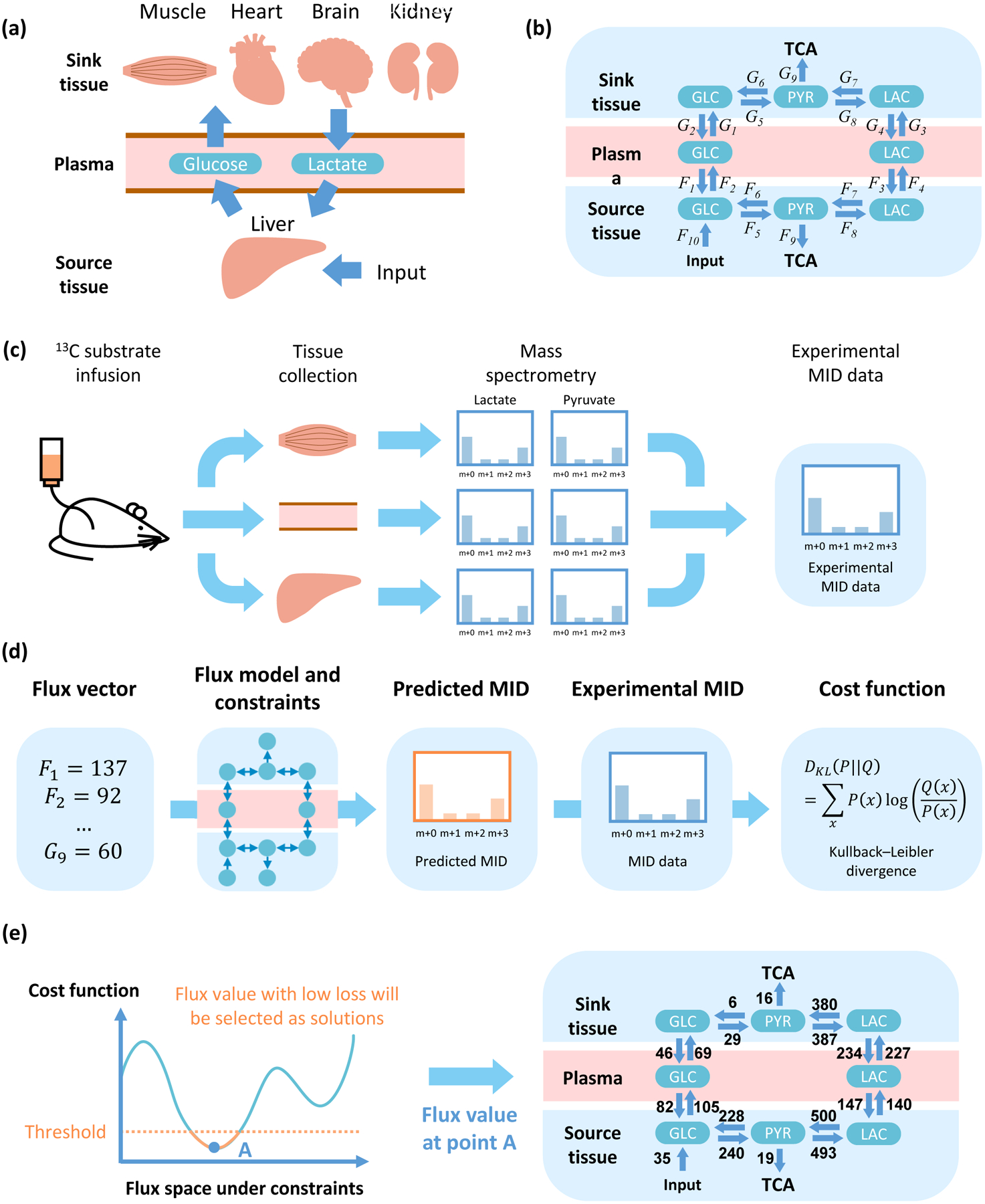
(a) Diagram of metabolite exchange between source and sink tissues. Glycogen, amino acids and other nutrition source are utilized to supplement glucose in the source tissue. (b) Three components (source tissue, plasma and sink tissue) and two circulating metabolites (lactate and glucose). (c) Data acquisition. Tissues of ¹³C-infused mice are extracted and analyzed by mass spectrometry. Distribution of mass isotopomers for metabolites, such as glucose, lactate and pyruvate, are used to solve for the fluxes (b). (d) Definition of cost function. The flux vector is used to predict MID of target metabolites, and compared with experimental MID to calculate cost function. (e) Schematic and example of a feasible solution. The solution with cost function lower than a threshold is considered as feasible solution and will be utilized in the following analysis.

Fluxes are computed based on data from mass spectrometry (MS) in ¹³C-glucose infused mice as follows. After infusion, tissues are collected and analyzed by MS. Metabolites with ¹³C at different positions are distinguished and their relative abundance is referred to as the mass isotopomer distribution (MID) (Figure 1C). MID data are then used to fit the fluxes in the model. Given a set of fluxes, MIDs are calculated and compared with experimental data. The difference (i.e. cost function) between the estimated MIDs and experiments, measured by a standard metric used in Information Theory, the Kullback-Leibler divergence (Kullback and Leibler, 1951), is minimized to find a set of fluxes that best fits the data. Next, statistical sampling is conducted to find all sets of fluxes that can be considered as valid solutions (Figures 1D, E, STAR Methods). Additional constraints are then introduced to ensure the simulated fluxes are physiological feasible, such as requirements for minimal TCA flux values in the source and sink tissues (STAR Methods).

The model was first fit and fluxes were computed using data from a recent study (Hui et al., 2017). Among all calculations of fluxes obtained from our algorithmic procedure (Figures 1C–E), the MIDs of most metabolites can be predicted by the current model (Figure S1A–H), and the values of the fluxes in the model are physiologically feasible (Figure S1I). The value of the cost function for the set of fluxes computed is also significantly lower that what is obtained from considering randomized data indicating that the values of fluxes computed are statistically significant (methods, Figure S1J–P).

Glucose contributions in different tissues

The flux network can be mathematically defined with a simplified diagram: the TCA cycle in the source and sink tissue is fed by two fluxes from glucose and lactate in plasma (Figure 2A, STAR Methods). Non-negative contribution fluxes to TCA cycle from glucose (F_glc in source tissue and G_glc in sink tissue) or from lactate (F_lac in source tissue and G_lac in sink tissue) are calculated from net fluxes of related reactions and diffusion (STAR Methods). From the computed fluxes, two glucose contribution ratios, a local one R_glc and a global one $R_{glc}^{\prime }$, are defined to reflect the relative ratio of glucose contribution to the TCA cycle. The local value R_glc distinguishes the glucose flux from circulating metabolites into the sink tissue and from the source tissue, while the global ratio $R_{glc}^{\prime }$ reflects the general glucose contribution in the complete model, which includes both sink and source tissue. If R_glc or $R_{glc}^{\prime }$ is higher than 0.5, it implies that glucose contributes more than lactate to TCA cycle in sink tissue or in the complete model, respectively. On the contrary, if it is lower than 0.5, lactate contributes more than glucose (Figure 2B, S2A).

Figure 2. Contribution to the TCA cycle from circulating glucose.

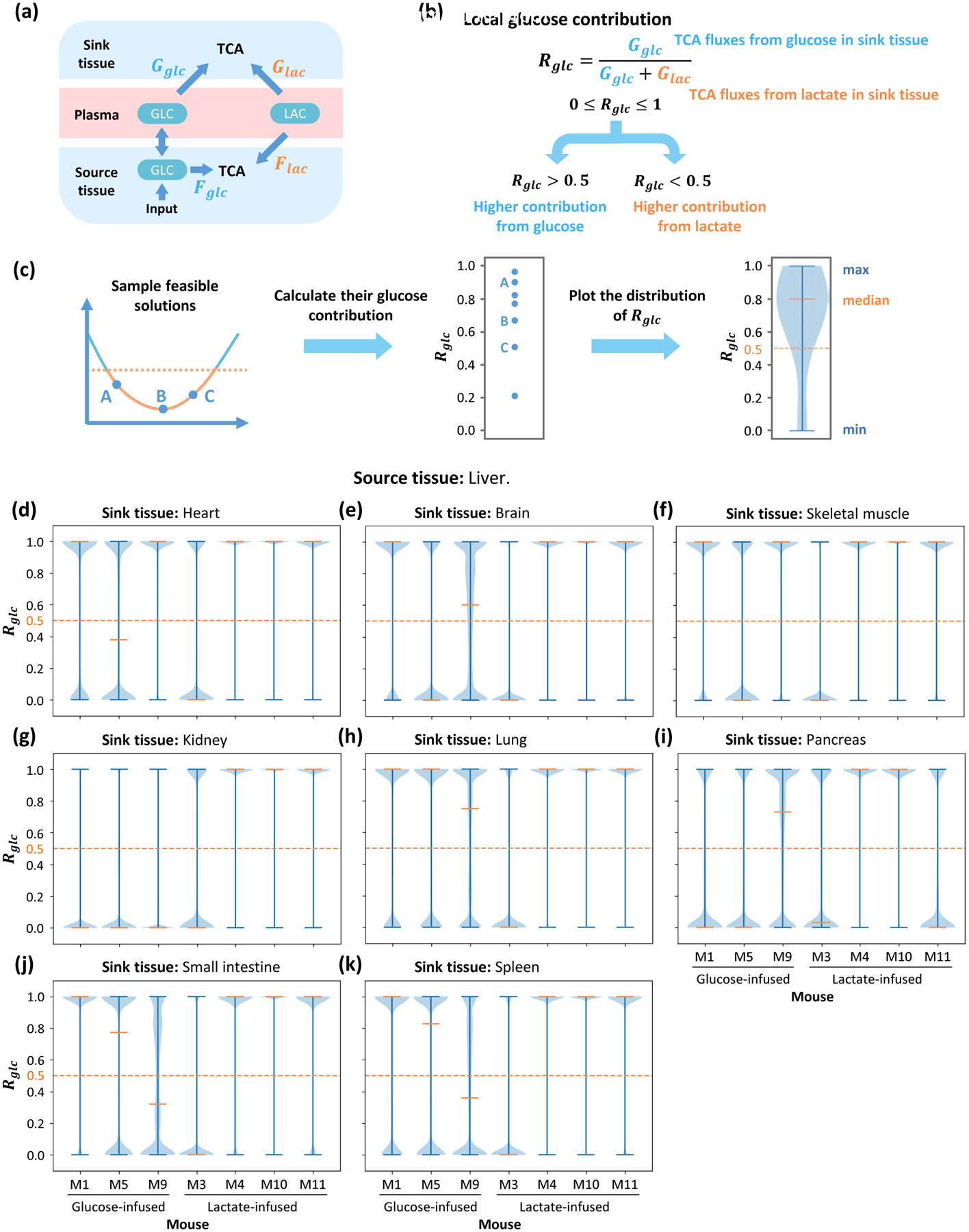
(a) Diagram of contribution fluxes. Glucose and lactate contribute to the TCA cycle by F_glc and F_lac in the source tissue, while G_glc and G_lac are related to the sink tissue. The direction of net flux between circulating glucose and glucose in source tissue is variable in different solutions. (b) Definition of global glucose contribution ratio R_glc based on fluxes in (a). The global glucose contribution R_glc is defined as the relative ratio of glucose contribution flux to total contribution flux in sink tissue. R_glc is a scalar between 0 and 1, and higher R_glc represents higher glucose contribution to the TCA cycle. (c) Procedure to compute distribution of glucose contribution. Feasible solutions are sampled and glucose contribution ratios are calculated. The distribution of glucose contribution is displayed by a violin plot. (d-k) Distribution of local glucose contribution based on models with different sink tissues. For each sink tissue, the source tissue is liver, and contribution ratio is calculated from data in 7 different mice. For most kinds of sink tissue, the median of glucose contribution is higher than 0.5 in most mice, which means glucose contributes more than lactate to the TCA cycle. The orange dash line represents 0.5 threshold. Data set is from glucose-infused mice (M1, M5, M9) and lactate-infused mice (M3, M4, M10, M11) in Hui et al, 2017.

To evaluate the glucose contribution, feasible solutions are sampled from the solution space and displayed in a violin plot (Figure 2C). The source tissue is the liver and the sink tissues are set as heart, brain, skeletal muscle, kidney, lung, pancreas, small intestine and spleen. For each combination of sink and source tissue, the model is fitted with data from mice infused by glucose and lactate. The local glucose contribution ratios R_glc tend to locate in extreme values in sampled feasible solutions and display a bimodal distribution (STAR Methods). In the fitted results, they largely concentrate around 1 in most of infused mice when fitting with different types of sink tissue (Figure 2D–K). The global glucose contribution ratios $R_{glc}^{\prime }$ show continuous distributions, and the median of the distribution in all types of sink tissue is higher than 0.5 (Figure S2B–I). Therefore, those results show that in almost all cases glucose contributes more than lactate does to the TCA cycle.

The results from these two-tissue models rely on MID data and some parameters. To evaluate these dependencies, we implemented a Monte Carlo based sensitivity analysis (Shestov et al., 2014). First, original data and parameters are perturbed randomly. The perturbed values are used to calculate distribution of the local contribution R_glc as previously described. After this process, the median of this distribution under each individual perturbation is collected, and the distribution of median R_glc reflects its sensitivity to data and parameters (Figure 3A). Results show that the median value of R_glc is very robust to perturbations in glucose circulatory flux and input flux, but more sensitive to the value of lactate circulatory flux and the MID data (Figure 3B–E). However, in most parameter sets, the median R_glc is still higher than 0.5 (Figure 3C, 3E). These results demonstrate the robustness of the conclusion that glucose contributes more than lactate to the TCA cycle under physiological conditions.

Figure 3. Parameter sensitivity analysis.

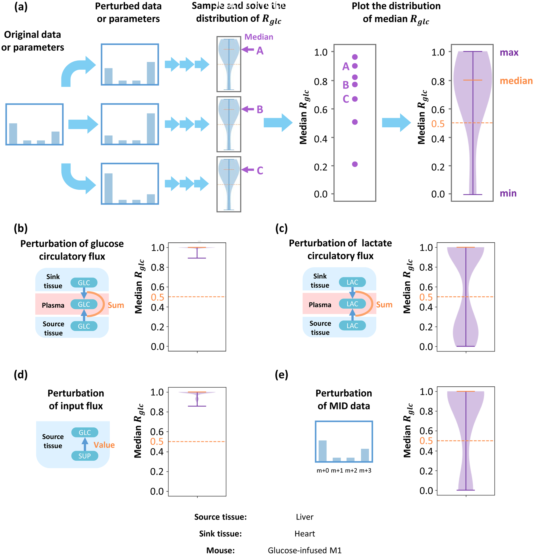
(a) Original MID data or constraint parameters are randomly perturbed and used in the following analysis. The resulting distribution of the local glucose contribution for each perturbation is calculated, and their medians are collected. Distribution of medians reflects parameter sensitivities for this model. The distribution of medians under perturbation of glucose circulatory flux (b), lactate circulatory flux (c), input flux in source tissue (d) and MID data (e). Although the local contribution ratio is more sensitive to lactate circulatory flux and MID data, most of the medians are above the 0.5 threshold, which implies that under most perturbations, glucose contributes more than lactate to the TCA cycle. Data set is from glucose-infused mouse M1 in Hui et al, 2017. Source tissue is liver and sink tissue is heart.

One confounding issue is that the process of tissue harvesting may induce ischemia and hypoxia. Hypoxia will induce elevated glycogenolysis in source tissue and glycolysis in sink tissue, which may significantly change measured MID of metabolites (Figure S3A). To estimate its effect on the final conclusion, a correction is introduced to simulate these effects under hypoxia. Measured MIDs of glucose in source tissue and lactate in sink tissue are assumed to be a mixture of 80% real MID in physiological state, and 20% MID of newly synthesized metabolites in elevated reactions under hypoxia (Figure S3B). Specifically, glucose in source tissue is assumed to be mixed with unlabeled glucose, and lactate in sink tissue is assumed to be mixed with lactate synthesized from pyruvate, which has same MID as pyruvate. Therefore, the physiological MID can be solved for and utilized for the same analysis of glucose contribution. Compared to results before the correction, conclusions were not altered, and in most cases glucose contributes more than lactate is robust to hypoxia considerations (Figure S3C–D).

Generality of the glucose contribution to the TCA cycle

To further investigate the generality of this conclusion, we considered a different animal strain, different diet and different infusion protocol with mice infused with ¹³C-glucose at a higher infusion rate which is one of the key technical variables of consideration in these studies (Ayala et al., 2010). In addition to our analysis of published data (Hui et al., 2017), these new experiments expand the scope of physiological variables (Figure 4A). These data are referred to as “high-infusion rate”, while the previous analysis is referred to as “low-infusion rate”. Importantly, with the higher infusion rate, the glucose, lactate and insulin levels in plasma are not significantly altered during the infusion (Figure 4B). Because of the higher infusion rate, an input flux J_in in plasma is added to the model to capture the infusion operation (Figure 4C). The amount of ¹³C labeling increases with the infusion rate, and with a higher infusion rate, the model predicts the MIDs (Figure S4A). In this case, the cost function is also significantly lower than that obtained from a random unfitted control for the 4 glucose-infused mice in the higher infusion rate experiments (Figure 4D), and the value of all fluxes are physiologically feasible (Figure S4B). As defined previously, the local contribution R_glc and global contribution $R_{glc}^{\prime }$ to the TCA cycle are calculated for the pair of source tissue (liver) and sink tissue (skeletal muscle) for all mice (Figure 4E, S4C). The analysis shows that in most mice, R_glc and $R_{glc}^{\prime }$ are both higher than 0.5, again implying that glucose contributes more than lactate to the TCA cycle (Figure 4F, S4D).

Figure 4. Robustness of results regarding animal strain and infusion rate.

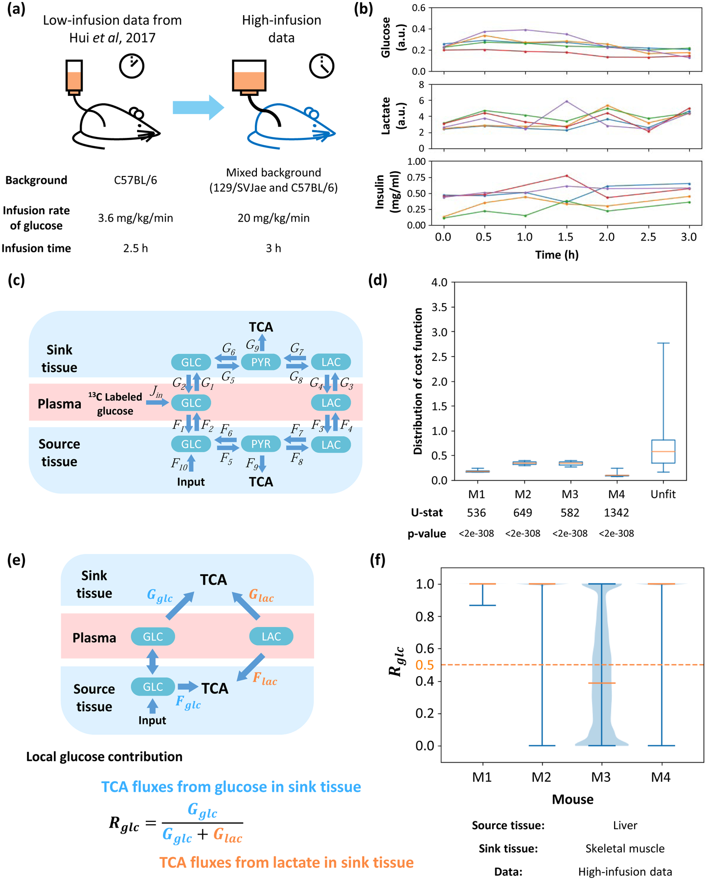
(a) Diagram of comparison between two experiments. A higher infusion rate and longer infusion time are introduced, which leads to higher abundance of ¹³C labeling in most metabolites. The genetic background and diet are also different from previous experiments. (b) Time-course data for concentrations of glucose, lactate and insulin in plasma during infusion. Each color represents a specific mouse. In the insulin measurement, a data point at 1h of red line is removed because of a significantly abnormal value. (c) Structure of high-infusion model. The main difference is ¹³C labeled infusion to glucose in plasma. (d) Distribution of cost function fitted with data from different mice or unfitted control data. U-statistics of a rank-sum test and p-values are displayed. (e) Definition of local glucose contribution R_glc. Glucose and lactate in plasma contribute to the TCA cycle in the source and sink tissue. Direction of net flux between circulating glucose and glucose in source tissue is variable in different solutions. The local glucose contribution R_glc is defined as the relative ratio of glucose contribution flux to total contribution flux in sink tissue. (f) Distribution of local glucose contribution shows glucose contributes more than lactate to the TCA cycle in most cases. Fits from different mice are displayed. In all subfigures, the source tissue is liver and sink tissue is skeletal muscle.

Glucose contribution upon consideration of multiple tissue interactions

The current model is based on source and sink tissues. However, mammals consist of tens of different tissues which cooperate and interact. To demonstrate the utility of this model to multiple tissue compartments, more sink tissues are introduced and the glucose contribution under these conditions are analyzed. This model contains one source tissue and two sink tissues, which are connected by glucose and lactate in plasma (Figure 5A, 5B). This model is fit with the low-infusion rate data, in which source tissue is liver and two sink tissues are combinations from heart, brain and skeletal muscle. The fitting is sufficiently precise (Figure S5A), implying that computed fluxes are physiologically feasible (Figure S5B). The cost functions of all combinations are also significantly lower than a random unfitted control (Figure S5C). In this model, glucose and lactate in plasma can contribute to the TCA cycle through three kinds of tissue, and therefore the definitions of local and global glucose contribution ratios R_glc and $R_{glc}^{\prime }$ are slightly modified (Figure 5C, S5D). Fitting results show in all three combinations of two sink tissues, glucose contributes more than does lactate to the TCA cycle regardless of the definition of glucose contribution ratio (i.e. local or global contribution ratio) used (Figure 5D, S5E).

Figure 5. Flux analysis across multiple tissues.

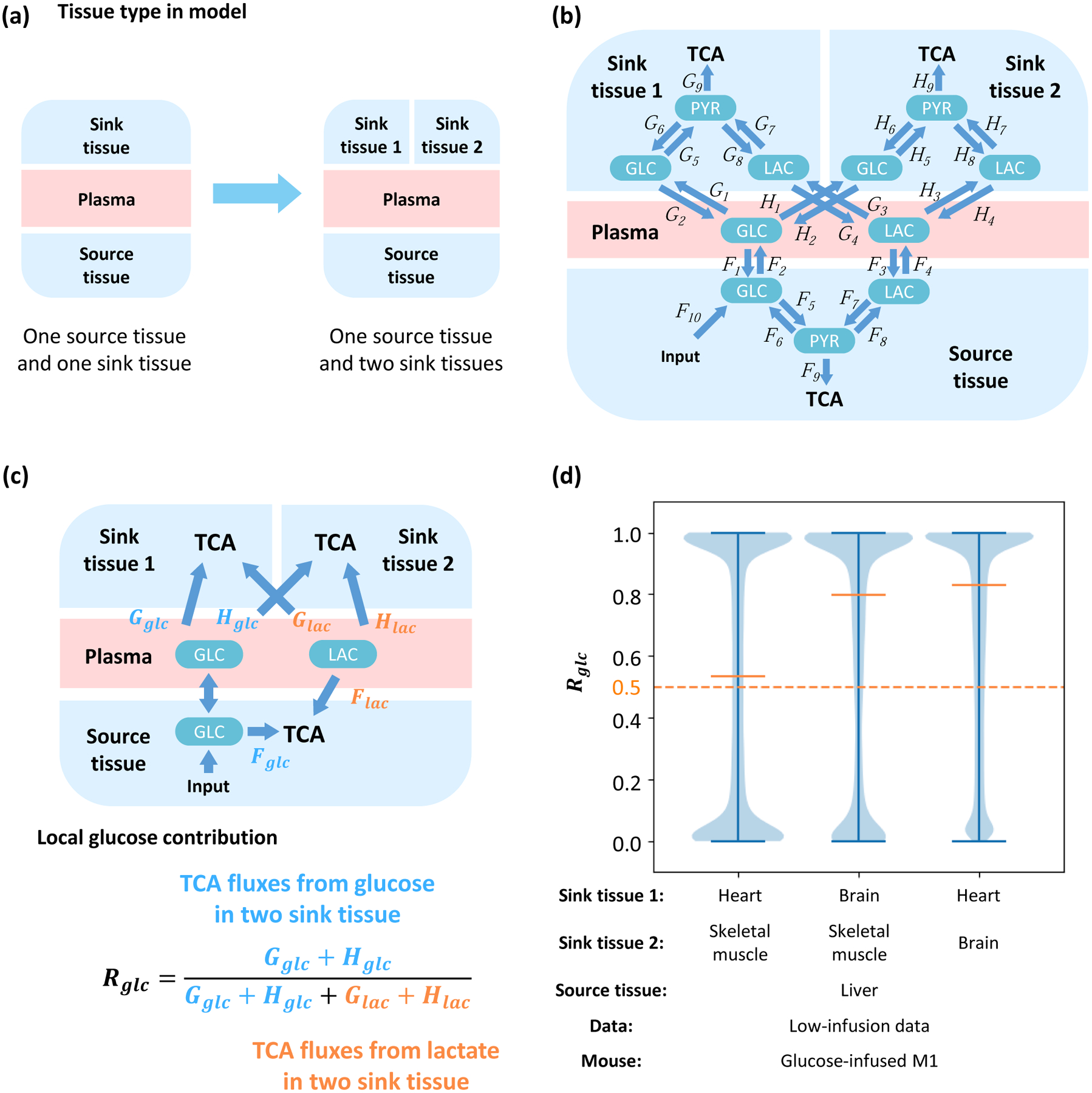
(a) A model with additional sink tissues. (b) Structure of the multi-tissue model. One source tissue and two sink tissues are connected by glucose and lactate in the plasma. (c) Definition of local glucose contribution R_glc. Glucose and lactate can contribute to TCA by F_glc and F_lac in the source tissue, G_glc and G_lac in the sink tissue 1, and H_glc and H_lac in sink tissue 2, respectively. Direction of net flux between circulating glucose and glucose in source tissue is variable in different solutions. The local glucose contribution is defined as the relative ratio of glucose contribution flux to total contribution flux in two kinds of sink tissue. (d) Distribution of local glucose contribution shows glucose contributes more than lactate to the TCA cycle in all combinations of sink tissues. The model is fit by glucose-infused mouse M1 from the low-infusion data in Hui et al, 2017. The source tissue is liver and the sink tissue 1 and 2 are two from heart, brain and skeletal muscle respectively.

Glucose contribution upon consideration of multiple nutrient sources

The current analysis considers two circulating metabolites as sources for the TCA cycle: glucose and lactate. However, many other metabolites circulate and are exchanged between tissue and plasma, such as acetate, alanine and pyruvate (Hui et al., 2017; Liu et al., 2018). Therefore, to investigate the applicability of this model, circulating pyruvate is introduced (Figure 6A). Circulating pyruvate can also represent other nutrient sources including but not limited to alanine, glutamine, acetate, or fatty acids. In this model, circulating pyruvate is not only exchanged with sink and source tissue, but also converted to lactate in plasma. Glucose and lactate in plasma can also be directly converted to pyruvate (Figure 6B). This model predicts the experimental MID with both low-infusion rate and high-infusion rate data (Figure S6A, S6B) with the physiologically feasible fluxes (Figure S5C, S5D). The distribution of values of the cost function is also significantly lower than random unfitted control in all kinds of sink tissue fitted with the low-infusion data (Figure S6E), or in the skeletal muscle fitted with the high-infusion data indicating statistical significance (Figure S5F).

Figure 6. Model with multiple circulating metabolites feeding the TCA cycle.

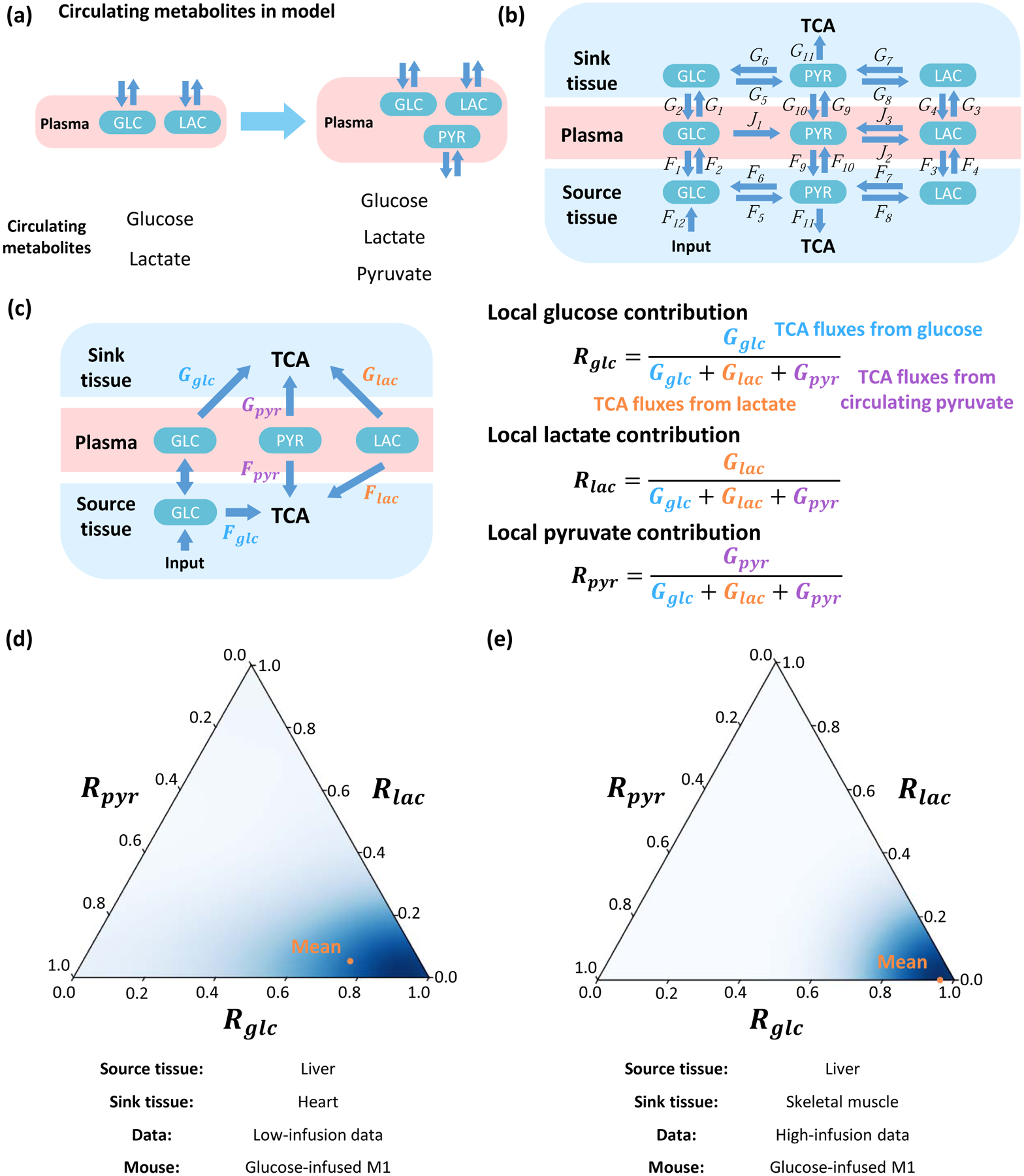
(a) Incorporation of additional circulating metabolites. (b) The structure of the model. The source tissue and sink tissue are connected with glucose, lactate and pyruvate in the plasma. (c) Definition of local contribution from metabolites R_glc, R_lac and R_pyr. Glucose, lactate and pyruvate can contribute to the TCA cycle by F_glc, F_lac and F_pyr in source tissue, and G_glc, G_lac and G_pyr in the sink tissue. Direction of net flux between circulating glucose and glucose in source tissue is variable in different solutions. The local contribution ratios of three metabolites R_glc, R_lac and R_pyr are defined by the relative ratio of the contribution flux from each metabolite to total contribution flux of all three metabolites in sink tissue. (d) Ternary plot to display distributions of local contributions from three metabolites. The orange point indicates average level. The model is fit by glucose-infused mouse M1 from low-infusion data. The source tissue is liver and sink tissue is heart. (e) Analysis and results as in (d) but for additional high-infusion system of different animal strain, different diet and different infusion protocol. The model is fitted by glucose-infused mouse M1 from the high-infusion data. The source tissue is liver and sink tissue is skeletal muscle.

Because circulating glucose, lactate and pyruvate each contributes to the TCA cycle in source and sink tissues, the local contribution ratios of the three metabolites R_glc, R_lac and R_pyr need to be calculated individually, as well as three global contribution ratios $R_{glc}^{\prime }$, $R_{lac}^{\prime }$ and $R_{pyr}^{\prime }$, and the sum of the three local or global contribution ratios equals to 1 (Figure 6C, S6H). The distribution of three ratios can be displayed by a ternary plot (Marc et al., 2019, STAR Methods). For the low-infusion rate data, the local contribution from glucose is predominantly higher than lactate and pyruvate (Figure 6D), and the conclusion is similar when the sink tissue in the model is replaced by other types of tissue (Figure S6G). For the global contribution, contribution from glucose is close to or slightly lower than lactate, which are both significantly higher than pyruvate (Figure S6I). The situation is similar in the high-infusion rate data, in which the local contribution from glucose markedly dominates in all sampled solutions, but the global contribution from glucose is closed to lactate (Figure 6E. S6J). Therefore, in a model with more metabolites in circulatory system, circulating glucose contributes more than lactate to the TCA cycle in all kinds of sink tissue, and has similar contribution than does lactate.

DISCUSSION

The nutrient sources for the TCA cycle have long been of interest. However, due to difficulties in data acquisition and mathematical analysis, quantitative studies under physiological conditions are still rare. With advances in mass spectrometry and mathematical modeling, in vivo flux analysis studies with isotope-labeling data have become a mainstay in the study of metabolic physiology. Previous studies have measured TCA cycle source utilization by MFA. However, with the development of these new mathematical tools, our study challenges some key conclusions that form the current consensus for the relative contributions of lactate and glucose to the TCA cycle. For example, it was reported that lactate is the major energy source for most tissues and tumors (Hui et al., 2017; Jin et al., 2019). Our results show that most organs uptake more glucose than lactate to fuel the TCA cycle. This conclusion also holds under various parameters, experimental conditions such as animal strain and diet, tissue type, tissue interactions and source metabolite number, which together indicate the robustness and generalizability of the conclusions. Our results, however, are consistent with conventional knowledge that glucose behaves as a primary energy source in cells and tissues, especially for neural systems (Nelson et al., 2017). Nevertheless, our results confirm that lactate is highly exchanged between tissue and plasma, while glucose is transferred from the liver to other organs. These phenomena appear to also be observed in recent studies on flux measurements in pigs (Jang et al., 2019).

In addition to addressing an important issue in metabolic physiology, our study provides a framework for metabolic flux analysis in physiological conditions. Compared with previous studies, the first improvement is that fluxes calculated by our model can capture more aspects of metabolic biochemistry. For example, the flux from pyruvate to glucose (G6/H6), the gluconeogenesis flux in sink tissue, relies on Phosphoenolpyruvate Carboxykinase (PEPCK), which only expresses in few kinds of tissue such as liver, kidney and adipose tissue (Geiger et al., 2013). Therefore, G6/H6 fluxes are very small in most of our fitting results (Figure S1I, S4B, S5B, S6C–D). Another example is high diffusion and exchange of lactate between tissue and plasma, which is usually overlooked, but captured by our model (F3/F4, G3/G4, H3/H4 in Figure S1I, S4B, S5B, S6C–D) and validated by experimental measurements (Jang et al., 2019). The second improvement is that, rather than fitting the model with a single solution, we sampled the entire high-dimensional solution space and analyzed all feasible results. Those millions of sampled points can cover more regions in solution space and precisely reflect real distribution of fluxes, especially in a complicated model. The third improvement is more complete analysis for parameter sensitivity than previous studies. This study verified the robustness of the conclusions not only under random perturbation of parameters and MID data, which accounts for uncertainties in experimental precision, but also may account for hypoxia which introduces systematic experimental bias. These analyses serve to extend much of the Metabolic Flux Analysis framework that was developed for cell systems to physiological conditions.

Another intriguing feature of this model is its generalizability and scalability. From a basic two-tissue version, this model is readily extended to compute fluxes from isotope patterns with higher infusion rates, more tissue types and more nutrient sources which could be useful to study for example different nutritional situations and pathophysiology states such as metabolic syndromes, diabetes and cardiovascular disease. The generality of this model allows for a broader usage in future research. More kinds of tissue can be introduced to better mimic the physiological condition such as the interaction between cancer and host organs. As the number of tissues considered increases, their roles could be more complicated rather than a single source and sink. For example, previous research indicates that the kidney may also have a significant contribution to net production of glucose in pigs (Jang et al., 2019). Second, more nutrient sources could be introduced and the metabolic network in each cell could also be expanded. The current model includes three nodes: glucose, pyruvate and lactate which capture fluxes in central carbon metabolism but could be extended into intermediary metabolism. Although sufficient for analyzing the contribution of macronutrients, studies of fatty acids, ketosis and amino acid metabolism will require a larger network. Nevertheless, the methodology contained within this model could be extended. For instance, subcellular compartmentalized metabolic flux analysis is also important (Lee et al., 2019). However, its application is usually restricted to the mitochondria and nucleus because of the difficulty in acquiring isotope-labeling data in each cellular compartment. On the other hand, interactions within heterogenous tissues could also be described by this model. It has been widely shown that cells in a tumor may express different metabolic states, and will compete or cooperate for many resources (Hensley et al., 2016). Quantitative methods based on this model may help to better describe those precise and complicated interactions.

LIMITATIONS OF STUDY

Our ability to resolve metabolic fluxes is first limited by the data. Thus, limited by data and then computational techniques, this model only covers a small portion of biochemical reactions. Specifically, this model combines all fluxes in the TCA cycle into one unidirectional flux that gives an overall rate, because adding those fluxes and metabolites to the model will not largely improve fitting precision of current fluxes, but will increase the dimension of solution space and thus increase uncertainty of results (STAR Methods). Therefore, this model may not fit the MID of some metabolites connected with TCA. For example, pyruvate can feed the TCA cycle and change the MID of metabolites in it, but it can also be fed by cataplerotic fluxes of TCA cycle. Consequently, the MID of pyruvate will be coupled with metabolites in TCA cycle, and cannot be precisely described as the model currently stands. Another limitation is the high dimensionality of the solution space in light of limited available constraints. In our models, high dimensionality of the solution space requires sampling algorithms to measure the solution space. As the model expands, these algorithmic challenges become more difficult. Thus, more constraints must be introduced to reduce the dimensionality of the feasible solution space. For example, our study includes constraints from circulatory fluxes (Hui et al., 2017), and some MFA model uses fixed biomass fluxes as boundary conditions (Reid et al., 2018). However, the precision and generalizability of these external constraints requires additional assessments, and they may introduce bias. Heterogeneity of those constraints in different individual systems should also be evaluated. Comprehensive and precise model analysis requires more effort to establish reliable constraints as well as acquisition of metabolite data with more coverage and higher resolution.

STAR METHODS

RESOURCE AVAILABILITY

Lead Contact

Further information and requests for reagents may be directed to and will be fulfilled as appropriate by the Lead Contact, Jason W. Locasale (dr.jason.locasale@gmail.com).

Materials Availability

This study did not generate new unique reagents.

Data and Code Availability

The low-infusion data set is available in previous work (Hui et al., 2017). The time-series concentration data of metabolites in plasma, the high-infusion data set and all source codes are available from GitHub (https://github.com/LocasaleLab/Lactate_MFA). Scripts in this study are implemented in Python 3.6. The package version dependency is also provided on GitHub website. A Docker on Linux system for out-of-the-box running is also available on Docker Hub (https://hub.docker.com/r/locasalelab/lactate_mfa). Each model requires around 10 ~ 50 hours of running time.

EXPERIMENTAL MODEL AND SUBJECT DETAILS

Animal

All animal procedures were approved by the Institutional Animal Care and Use Committee (IACUC) at Duke University. Mouse models is from 8 to 10-week old, male and female mixed background (129/SVJae and C57BL/6) with a combination of alleles that have been previously described: Pax7^CreER-T2, p53^FL/FL, LSL-Nras^G12D and ROSA26^mTmG (Zhang et al., 2015). Mice were fed standard laboratory chow diets ad libitum.

METHOD DETAILS

Data Sources

This study is based on two data sources: low-infusion data were obtained from infused fasting mice in previous work (Hui et al., 2017), while the high-infusion data were acquired based on following protocols.

Reagents

Unless otherwise specified, all reagents were purchased from Sigma-Aldrich. Jugular vein catheters, vascular access buttons, and infusion equipment were purchased from Instech Laboratories. Stable isotope glucose were purchased from Cambridge Isotope Laboratories.

In vivo ¹³C glucose infusions

To perform in vivo nutrient infusions, chronic indwelling catheters were placed into the right jugular veins of mice and animals were allowed to recover for 3–4 days prior to infusions. Mice were fasted for 6 hours and infused with [U-13C]glucose for 3 hours at a rate of 20 mg/kg/min (150 μL/hr). Blood was collected via the tail vein at 3 h and serum was collected by centrifuging blood at 3000g for 15 min at 4°C. At the end of infusions, tissues were snap frozen in liquid nitrogen and stored at −80°C for further analyses.

Insulin measurement

The concentration of insulin in plasma is measured by Ultra Sensitive Mouse Insulin ELISA Kit from Crystal Chem.

Metabolite extraction from tissue

Briefly, the tissue sample was first homogenized in liquid nitrogen and then 5 to 10 mg was weighed in a new Eppendorf tube. Ice cold extraction solvent (250 μl) was added to tissue sample, and a pellet mixer was used to further break down the tissue chunk and form an even suspension, followed by addition of 250 μl to rinse the pellet mixer. After incubation on ice for an additional 10 min, the tissue extract was centrifuged at a speed of 20 000 g at 4 °C for 10 min. 5 μl of the supernatant was saved in −80 °C freezer until ready for further derivatization, and the rest of the supernatant was transferred to a new Eppendorf tube and dried in a speed vacuum concentrator. The dry pellets were reconstituted into 30 μl (per 3 mg tissue) sample solvent (water:methanol:acetonitrile, 2:1:1, v/v) and 3 μl was injected to LC-HRMS.

HPLC method

Ultimate 3000 UHPLC (Dionex) was used for metabolite separation and detection. For polar metabolite analysis, a hydrophilic interaction chromatography method (HILIC) with an Xbridge amide column (100 × 2.1 mm i.d., 3.5 μm; Waters) was used for compound separation at room temperature. The mobile phase and gradient information were described previously. 2-hydrazinoquinoline derivatives were measured using reversed phase LC method, which employed an Acclaim RSLC 120 C8 reversed phase column (150 × 2.1 mm i.d., 2.2 μm; Dionex) with mobile phase A: water with 0.5% formic acid, and mobile phase B: acetonitrile. Linear gradient was: 0 min, 2% B; 3 min, 2% B; 8 min, 85% B;9.5 min, 98% B; 10.8 min, 98% B, and 11 min, 2% B. Flow rate: 0.2 ml/min. Column temperature: 25 °C.

Mass Spectrometry

The Q Exactive Plus mass spectrometer (HRMS) was equipped with a HESI probe, and the relevant parameters were as listed: heater temperature, 120 °C; sheath gas, 30; auxiliary gas, 10; sweep gas, 3; spray voltage, 3.6 kV for positive mode and 2.5 kV for negative mode. Capillary temperature was set at 320°C, and S-lens was 55. A full scan range was set at 70 to 900 (m/z) with positive/negative switching when coupled with the HILIC method, or 170 to 800 (m/z) at positive mode when coupled with reversed phase LC method. The resolution was set at 140 000 (at m/z 200). The maximum injection time (max IT) was 200 ms at resolution of 70 000 and 450 ms at resolution of 140 000. Automated gain control (AGC) was targeted at 3 × 106 ions. For targeted MS2 analysis, the isolation width of the precursor ion was set at 1.0 (m/z), high energy collision dissociation (HCD) was 35%, and max IT is 100 ms. The resolution and AGC were 35 000 and 200 000, respectively.

Metabolite Peak Extraction and Data Analysis

Raw peak data was processed on Sieve 2.0 software (Thermo Scientific) with peak alignment and detection performed according to the manufacturer’s protocol. The method “peak alignment and frame extraction” was applied for targeted metabolite analysis. An input file of theoretical m/z and detected retention time was used for targeted metabolite analysis, and the m/z width was set to 5 ppm. An output file was obtained after data processing that included detected m/z and relative intensity in the different samples.

QUANTIFICATION AND STATISTICAL ANALYSIS

GENERAL ANALYSIS METHOD

Model design

A principle of model design is parsimony, also referred to as “Occam’s razor” that is to use the simplest model that can appropriately address the question at hand. Inclusion of parameters and variables should correspond to available data and constraints that parameterize the model and allow for the model to address the relevant questions. The primary goal of this study is to quantify the contribution of circulating glucose and lactate to the TCA cycle. Therefore, the model, to reach appropriate conclusions, should balance the ability to achieve this goal and the complexity that can be precisely evaluated from available data.

To study circulating metabolites, the model contains at least two compartments: plasma and a specific tissue. However, because circulating glucose and lactate must be balanced, the net flux between plasma and tissue is limited to boundary fluxes of circulating glucose and lactate, which cannot capture dynamics between circulation and target organs. Therefore, a heterogenous two tissue system is introduced, and it allows for different patterns in utilization of nutrient source. One common pattern is the Cori cycle, in which in the fasting state, the sink tissue (muscle) utilizes circulating glucose and excretes lactate, while the source tissue (liver) convert them back to glucose. The basic structure using two tissues and plasma is already difficult to model. To prevent overfitting leading to parameter uncertainty, the network in each tissue contains three key nodes: glucose, pyruvate and lactate, and their interconversion fluxes. TCA-related reactions are described by one unidirectional flux, because introducing more TCA cycle reactions would not address the question of relative nutrient contributions and lead to overfitting. To intuitively understand whether TCA-related reactions have a substantial impact on the labeling patterns, the MID of phosphoenolpyruvate (PEP), the metabolite generated from oxaloacetate (OAA) in the first step of gluconeogenesis, is also measured in liver (source tissue) and skeleton muscle (sink tissue) in the high-infusion rate data. The MID for PEP is uncorrelated with that of malate in TCA cycle (Figure S7A), suggesting that the cataplerotic flux from the TCA cycle intermediates to glucose (which requires PEP as an intermediate) does not have a significant impact on labeling patterns of metabolites. Similar results are also observed in a previous study from Hui et al Nature 2017. Although the MID of PEP is not available in those data, 3-phosphoglycerate (3PG), the metabolite adjacent to PEP in glycolysis/gluconeogenesis (Figure S7B), showed a similar trend, again indicating that the effect of the labeling pattern from TCA cycle intermediates to glucose is very low. Therefore, although previous studies show that cataplerotic flux of TCA may be one of major sources of PEP in liver, introducing more TCA reactions do change results of the fits from current metabolites, and thus not significantly improve the precision of this model.

However, a more complicated model that includes every reaction carrying the fluxes of the TCA cycle, at least 6 metabolite MIDs and tens of fluxes should be added, including citrate, α-ketoglutarate (as well as glutamate), succinate, oxaloacetate (as well as aspartate) in the TCA cycle and PEP in glycolysis. Absolute measurements of fluxes feeding into the TCA cycle from other carbon sources such as branched chain amino acids and glutamine are also required to fully parameterize the model. The lack of data would lead to overfitting and parameter uncertainty which limits the conclusions that can be drawn. Under this condition, introducing more detailed fluxes may not substantially improve fitting precision, but would introduce uncertainties within the current model. Therefore, after careful consideration of the available data and the primary goal of the model, the resulting model consists of one plasma and two tissues, which includes glucose, pyruvate, lactate and conversion fluxes between them.

There are some limitations in the current model. For example, in the source tissue, M+3 PEP is higher and M+3 pyruvate is lower compared with that in sink tissue. considering the similar abundance of M+6 glucose both in source and sink tissue (Figure S4A), this implies that there might be more high-labeled carbon source that supply of PEP in the source tissue. Limited by available data, the current model cannot explain the source of those hidden high-labeled carbon sources. Similarly, lower M+3 pyruvate in the source tissue might be due to some unlabeled sources of pyruvate in source tissue, such as glucogenic amino acids. However, data also show that the abundance of M+4 in malate in liver is very low, both in the Hui et al. Nature 2017 data and the high-infusion data. Considering the high exchange rate between malate and aspartate/oxalacetate, although the cataplerotic flux may be one of the main sources of PEP, it should not be the main reason for higher M+3 PEP in source tissue, nor the main reason of the difference between experimental and predicted MID in this study.

The structure of this model is another point of discussion. For example, in cellular metabolism, the flux G2 relies on glucose 6-phosphatase (G6Pase), but most kinds of sink tissue lack this enzyme. Similarly, the flux G6 relies on phosphoenolpyruvate carboxykinase (PEPCK), which is often thought to be most highly expressed in liver. However, these two fluxes are both preserved in the sink tissue, since one of the main goal of this model is to introduce exchange fluxes of some metabolites between tissue and circulation. Exchange fluxes may significantly affect MID data, which will also influences the results of flux analysis. In tissue level, these exchange fluxes are derived as an abstracted model of a series of complicated biochemical reactions, including transport in extracellular fluid, absorption/secretion by tissue cells, and utilization/production by the tissue cells. This complicated process is not directly equivalent to a cellular biochemical reaction. On the other aspect, for the G2 flux, many sink tissues, such as kidney, heart, lung, head and leg, has been reported to have release flux or nearly release flux of glucose by direct flux measurement in pigs (Figure 3B, 3C in (Jang et al., 2019)). For the G6 flux in sink tissue, from the distribution in the region of feasible solutions, G6 is very small in most cases (Figure S7I, M1 and M4 in Figure S4B, Figure S5B, Figure S6C–D). However, because of heterogeneity in biological organisms, in some cases G6 is still very high (M2 and M3 in Figure S4B). These results indicate that the current model may reflect the difference between cellular level and tissue/organ level metabolism.

Flux model

In this study, each metabolic reaction network includes many fluxes between different metabolites (chemical reactions) or metabolites traversing through different tissues (diffusions). Flux models include glucose, lactate and pyruvate as metabolites in three compartments (plasma, source tissue and sink tissue). Each model contains tens of fluxes, labeled with F (for fluxes in the source tissue), G (for fluxes in the sink tissue), H (for fluxes in the second sink tissue in models with multiple sink tissues) and J (for fluxes within plasma). The solution is a vector F = {F₁, F₂,…, G₁, G₂,…H₁,…, J₁,…} containing flux values for all reactions in the metabolic reaction network.

It is required that all fluxes satisfy mass balance constraint, which is:

$$\sum _{\forall F_{in,i}}{F}_{in,i}=\sum _{\forall F_{out,i}}{F}_{out,i}$$ (S1)

in which F_in,i and F_out,i represent all input and output fluxes connected to metabolite i respectively (Figure S7C). All fluxes are required to be within a range [F_min, F_max].

Flux constraints

To reduce the degrees of freedom, constraints are introduced: first, the flux that supplements glucose in the source tissue (referred as F₁₀ in all models) is set as a fixed value F_input. Second, the sum of total input fluxes to plasma glucose, which is glucose turnover flux in plasma, is set as a fixed value F_circ,glc. Similarly, the lactate turnover flux in plasma is set as a fixed value F_circ,lac (Figure S7D). Their values were chosen from previous research (Hui et al., 2017), and sensitivity with respect to changes in their values was evaluated.

To search the solution space, some fluxes are set to a fixed value during the fitting process. Details are explained in “Solution space sampling” section.

Mass isotopomer distribution calculation

The predicted mass isotopomer distribution (MID) of a metabolite is calculated based on MID of its precursors and corresponding flux values, which can be expressed as:

$${\tilde{M}}_i=\frac{\sum _j{F}_j{M}_{ji}}{\sum _j{F}_j}$$ (S2)

where ${\tilde{M}}_i$ is predicted MID of metabolite i, M_ji is MID of metabolite i produced from a substrate j, and F_j is the flux from j to i. M_ji could be calculated by experimental MID of metabolite j: M_ji = f(M_j), in which f is the MID conversion function between substrate j and product i.

For example, glucose and lactate can be converted to pyruvate and mixed together. In the source tissue, F₅ and F₇ describes the fluxes that convert glucose and lactate to pyruvate, respectively. Therefore, the predicted MID of pyruvate in the source tissue that comes from lactate and glucose can be formulated (Figure S7E).

For the MID conversion function f, there are three types of conversions:

1. Transport of metabolites between plasma and tissue, such as metabolite j being glucose in the plasma and metabolite i being glucose in the source tissue. This conversion does not change the MID. Therefore, M_ji = M_j.

2. Conversion between lactate and pyruvate, such as metabolite j being lactate in the source tissue and metabolite i being pyruvate in the source tissue. Because they have similar structure, conversion between lactate and pyruvate does not change MID. Therefore, M_ji = M_j is also valid in this category.

3. Conversion between glucose and pyruvate, such as metabolite j being glucose in the source tissue and metabolite i being pyruvate in the source tissue. Because they have a different carbon number, this kind of conversion is complicated. Two special functions are designed to calculate the corresponding MIDs:

   1. To calculate the MID of glucose produced by pyruvate through gluconeogenesis, a convolution is used. Suppose that the MID of pyruvate is M_pyr = [M_pyr,0, M_pyr,1, M_pyr,2, M_pyr,3], the MID vector of glucose synthetized from pyruvate could be expressed as a convolution function:

      $${\mathit{M}}_{glc\_\mathit{\text{from}}\_pyr}=\mathit{\text{conv}}2\left(M_{pyr}\right)=\mathit{\text{convolution}}\left(M_{pyr},M_{pyr}\right)$$ (S3)

      where the discrete convolution function is defined as:

      $$\text{If}\text{two}\text{vectors}A=\left[A_0,\dots ,A_{m-1}\right]\text{and}B=\left[B_0,\dots ,B_{n-1}\right],$$

      $$C=\mathit{\text{convolution}}(A,B),\text{in which: }$$

      $$C_k=\sum _{i=\text{max}(0,k-n)}^{\text{min}(k,m-1)}{A}_i{B}_{k-i},k\in \left\{0,1,\dots ,m+n-1\right\}$$ (S4)
   2. To calculate the MID of pyruvate produced by glucose through glycolysis, an approximation method is used here. Suppose that the MID of glucose is M_glc = [M_glc,0, M_glc,1, M_glc,2, M_glc,3, M_glc,4, M_glc,5, M_glc,6], because for glucose, carbon atoms are either all ¹³C or all ¹²C, M_glc,0 and M_glc,6 will be dominant in MID vectors. Therefore, the MID of pyruvate from glucose could be expressed as a split function:

      $$M_{pyr}=\mathit{\text{split}}\left(M_{glc}\right)=\left[M_{glc,0},M_{glc,mid},M_{glc,mid}{M}_{glc,6}\right]$$ (S5)

      in which $M_{glc,mid}=\frac{1-M_{glc,0}-M_{glc,6}}{2}$
      The MID of unlabeled glucose is set to M_glc,natural, which is a binomial distribution based on the natural abundance of ¹³C in glucose, that is:

      $$M_{glc,\mathit{\text{natural}},i}=\left(\begin{array}{c}6\\ i\end{array}\right)R_{13C}^i{\left(1-R_{13C}\right)}^{6-i},i=0,1,\dots ,6$$ (S6)

      in which R_13C is natural abundance of ¹³C. The MID of infused labeled glucose (substrate of J_in flux in some models) is set to M_glc,label, in which all carbon atoms are ¹³C.

MID fitting and flux solutions

The flux solution to a MID data is obtained by minimizing the difference between predicted and experimental MID data. The difference between the predicted MID ${\tilde{M}}_x$ and the experimental MID M_x for a metabolite x can be defined by the Kullback–Leibler divergence D_KL (Kullback and Leibler, 1951), which is referred as cost function L_x:

$$L_x=D_{KL}\left({\tilde{M}}_x\parallel M_x\right)=\sum _i\left(M_{x,i}+{\epsilon }_{\text{log}}\right)\text{log}\frac{{\tilde{M}}_{x,i}+{\epsilon }_{\text{log}}}{M_{x,i}+{\epsilon }_{\text{log}}}$$ (S7)

in which M_x,i and ${\tilde{M}}_{x,i}$ are element i in vector M_x and ${\tilde{M}}_x$, respectively. ε_log is a small number added to maintain numerical stability.

The total cost function of a model is the sum of cost function values for selected metabolites (referred as target metabolites), which is defined as:

$$L_{\mathit{\text{model}}}=\sum _x{L}_x$$ (S8)

Target metabolites in most models consisting of glucose, pyruvate and lactate in source and sink tissues. Some models may include target metabolites in plasma for better fitting.

Because each ${\tilde{M}}_x$ is a function of the flux vector F, the cost function of the model L_model is also a function of F. Therefore, the flux solution can be written as:

$$\underset{F}{\text{min}}{L}_{mоdel}(F),\text{s.t.}A\cdot F=b\text{and}{F}_{\text{min}}\le F\le F_{\text{max}}$$ (S9)

in which A·F = b represents the flux balance requirement and other constraints. An additional constraint of a flux range F ∈ [F_min, F_max] is also incorporated.

Eq. S9 represents an optimization problem with a nonlinear objective function, linear equality and inequality constraints. Therefore, it is a constrained nonlinear optimization problem. In this study, we solve this problem by sequential quadratic programming (SQP) implemented in the SciPy package (Kraft, 1988).

Similar with other iterative optimization algorithms, this algorithm starts with an initial solution and iterates to find the locally optimal point. The initial solution is generated by a linear programming (LP) problem:

$$\underset{F}{\text{min}}{r}^T\cdot F,\text{s.t.}A\cdot F=b\text{and}{F}_{\text{min}}\le F\le F_{\text{max}}$$ (S10)

in which r is a uniformly distributed random vector in range [−0.4, 0.6] with the same size as F. This linear programming problem is solved by a simplex algorithm implemented in SciPy package (Dantzig, 2016; Winston et al., 2003).

Because SQP can only calculate a local optimum, the LP step is repeated n_{opt_repeat} times to generate multiple different initial values. These initial values are fed into the SQP step to fit the flux vector respectively, and the flux vector with lowest objective value is then chosen as the final result. Random solutions are generated by Linear Programming (eq. S10) as previously described. The objective function value is computed for each random solution. To evaluate the difference in objective function values between the computed solutions and the random solutions, a p-value is calculated from a nonparametric Wilcoxon rank-sum test implemented in the SciPy package.

Glucose contribution calculation

After fitting a set of fluxes from the MID data, we can use the results to calculate the relative contribution of different nutrients to the TCA cycle. For all models in this study, the contribution from each nutrient in each tissue can be regarded as one non-negative contribution flux, referred as F_glc, G_glc, etc. From those contribution fluxes, the total contribution R_x from one metabolite x is defined as:

$$R_x=\frac{F_x+G_x+H_x}{\sum _y{F}_y+\sum _y{G}_y+\sum _y{H}_y},H_x\text{may}\text{not}\text{exist}\text{in}\text{some}\text{models}.$$ (S11)

To calculate the non-negative contribution fluxes from raw flux result, we calculate all net fluxes that are connected to TCA cycle. Suppose those net fluxes are F_net,x, F_net,y and F_net,z, they could be positive or negative. We calculate the contribution fluxes from the following formulae:

$$F_{\mathit{\text{total}},in}=\sum _{\forall F_{net,x}>0}{F}_{net,x}$$ (S12)

$$F_{\mathit{\text{total}},out}=-\sum _{\forall F_{net,x}<0}{F}_{net,x}$$ (S13)

$$\text{For}\text{each}\text{metabolite}x:F_x=\{\begin{array}{cc}\left(1-\frac{F_{\mathit{\text{total}},out}}{F_{\mathit{\text{total}},in}}\right)F_{net,x}& F_{net,x}>0\\ 0& F_{net,x}<0\end{array}$$ (S14)

For example, suppose in a tissue, glucose, lactate and pyruvate can contribute to the TCA cycle. The raw fluxes are first converted to net fluxes F_net,glc, F_net,lac and F_net,pyr. Then, the non-negative absolute contribution fluxes F_glc, F_lac and F_pyr are calculated based on eq. S14. Finally, the normalized contribution ratio can be calculated from S11 (Figure S7F).

In the simple situation with only two metabolites (lactate and glucose), eq. S14 simplifies:

$$\text{If}{F}_{net,glc}>0,F_{net,lac}>0:F_{glc}=F_{net,glc}\text{and}{F}_{lac}=F_{net,lac}$$

$$\text{If}{F}_{net,glc}<0,F_{net,lac}>0:F_{glc}=0\text{and}{F}_{lac}=F_{net,lac}+F_{net,glc}$$

$$\text{If}{F}_{net,glc}>0,F_{net,lac}<0:F_{glc}=F_{net,glc}+F_{net,lac}\text{and}{F}_{lac}=0$$ (S15)

Solution space sampling

The dimension of the solution space in a model is calculated based on:

$$n_{dim}=n_{\mathit{\text{flux}}}-n_{\mathit{\text{balance}}}-n_{\mathit{\text{constrain}}}-n_{mid}$$ (S16)

in which n_flux is the number of flux variable, n_balance is the number of flux balance equations (number of eq. S1), n_constrain is the number of flux constraint equations, and n_mid is the number of MID equations used to fit the model (number of eq. S7 and also elements in eq. S8). n_dim equals to 2 in basic models (model A and model B) and is larger in the complicated model.

n_dim determines the degree of freedom in the solution space. To sample the solution space uniformly, values of some fluxes are fixed during fitting (or be constant in random unfitted solutions), and the number of fixed fluxes equals to n_dim. Those fluxes with fixed values are called “free fluxes”. Those free fluxes make the dimension of the solution space of the optimization problem the same as the number of target metabolites, which prevents the problem from being overdetermined or underdetermined. The values of free fluxes are added to flux constraints equation A · F = b during the optimization process.

Free fluxes are chosen based on model structure. In most models with n_dim equal to 2, fluxes F₁ and G₂ are chosen as free fluxes. The values of free fluxes are sampled uniformly in their defined ranges. When there are only two free fluxes, the whole solution space is scanned based on a lattice with n_lattice discrete values on each edge (totally $n_{\mathit{\text{lattice}}}^2$ points) (Figure S7G). As its dimension of free fluxes increases, computational cost for thorough scanning grows exponentially. Therefore, in some models with higher n_dim, we choose n_diag points with equal intervals on the diagonal of the solution space and shuffle their coordinates to cover the whole space (Figure S7H).

For each point of free fluxes, the LP problem is solved to obtain the initial solution. If no solution exists under the current free flux combination, this point will be discarded in the following calculation. After generating an initial solution, for the random unfitted solutions, it is directly returned for following analysis. For fitted solutions, the SQP algorithm is executed to obtain the final flux vector F* that minimizes the objective function (eq. S8) and the corresponding objective value L*. To be regarded as a feasible solution, F* must satisfy a series of requirements: First, F* should meet minimal requirement for the value of a TCA flux, which means that one or multiple TCA fluxes must be larger than a threshold F_TCA,min. Secondly, L* should be small enough, which means the predicted MID data based on F* is close enough to experimental data. Therefore, we require the objective value L* must be smaller than a threshold of objective function L_threshold. Only feasible solutions will be used to calculate the final distribution of glucose contribution. Therefore, the general procedure of glucose contribution analysis is shown as follows:

1. Choose the free fluxes based on the model.

2. Generate the sample of free fluxes in the solution space.

3. Optimize the objective function and solve for the corresponding flux values based on each free flux sample. Select those solutions with large enough TCA fluxes and small enough objective value.

4. Calculate glucose contribution for all feasible solutions.

5. Plot distribution of glucose contribution.

Parameter sensitivity

For a parameter sensitivity analysis, experimental MID data or those flux constraints are varied based on a Gaussian distribution to generate n_{param_sample} different sets. For each perturbed parameter set, a solution space sampling is executed, similar with other model, to calculate the distribution of glucose contribution. For each MID data perturbation, each experimental MID vector are multiplied with a random vector, which consists of variables with identical independent distributions, to generate raw new vector $M_{x,i,raw}^{\prime }$, that is:

$$M_{x,i,raw}^{\prime }=M_{x,i}\left(1+{\delta }_i\right),\text{in}\text{which}{\delta }_i\text{is}\text{i.i.d.}\text{and}{M}_{x,i}\text{is}i\text{-th element}\text{in}{M}_x$$ (S17)

δ_i follows the truncated Gaussian distribution N(0, σ_mid) in the range of [0.1, 0.9] and [−0.9, −0.1]. Then the new raw MID vector is normalized to generate the final perturbed MID vector $M_x^{\prime }$:

$$M_{x,i}^{\prime }=\frac{M_{x,i,raw}^{\prime }}{\sum _i{M}_{x,i,raw}^{\prime }},\text{in which}{M}_{x,i}^{\prime }\text{is}i\text{-th element in }{M}_x^{\prime }.$$ (S18)

The MID vector of different metabolites is multiplied by different random vector in one data perturbation. The perturbed data are used for the following glucose contribution analysis. Perturbation of other constraints is similar with MID data perturbation. In each perturbation, the target constraint is multiplied by a random variable, that is:

$$F_{\mathit{\text{input}}}^{\prime }=F_{\mathit{\text{input}}}(1+\delta )$$ (S19)

$$F_{\mathit{\text{circ}},glc}^{\prime }=F_{\mathit{\text{circ}},glc}(1+\delta )$$ (S20)

$$F_{\mathit{\text{circ}},lac}^{\prime }=F_{\mathit{\text{circ}},lac}(1+\delta )$$ (S21)

Similar with the MID data, δ follows the truncated Gaussian distribution N(0, σ_flux) in the range of δ_mid or δ_flux. The perturbed parameters are used for the following glucose contribution analysis.

Hypoxia correction

Tissue extraction introduces issues due to hypoxia. To estimate these effects to the final glucose contribution, a correction to the MID data is introduced to simulate this process. The hypoxic state includes two major events: glycogen breakdown in source tissue and elevated lactate generation in sink tissue (figure S3A). To correct for the effect of hypoxia, the current data is assumed to be measured under hypoxia, which means the current MID of metabolites is a mixture of that metabolite in the original tissue and product of activated reaction under the hypoxia state. Specifically, the MID of glucose in the source tissue is mixture of (1−a_mix) (80%) original glucose MID and a_mix (20%) hydrolyzed glucose from glycogen (unlabeled MID), and the MID of lactate in the sink tissue is mixture of (1−a_mix) (80%) original one and a_mix (20%) reductive product from pyruvate (same MID as pyruvate in sink tissue) (figure S3B). From this assumption we calculate putative original MIDs of these two metabolites. If there is any negative item in MID, assign all of them to ε_mid and re-nomalized each MID to ensure sum of them equals to 1. Use those processed MID to do the same fitting and calculation of glucose contribution as Model A.

Ternary graph plotting

In those models with three circulating metabolites, glucose, pyruvate and lactate can all contribute to the contribution to the TCA cycle. Therefore, the ternary graph is plotted to display the distribution of their relative contribution ratio in one figure. The ternary graphs are plotted using a python package, python-ternary (https://github.com/marcharper/python-ternary).

For each free flux sample, the contribution from glucose R_glc, from pyruvate R_pyr and from lactate R_lac are calculated based on eq. S14. Each triple set (R_glc, R_lac, R_pyr) in ternary space T corresponds to the contribution of one sample of a free flux set with objective value lower than threshold. To better display the distribution of contribution the set of three fluxes, those points are binned and used to make the density heatmap. as figure 5D and E. Because of the limitation of ternary plot package, a complicated protocol is designed to reflect the point density (Figure S7I).

First, those sets (R_glc, R_lac, R_pyr) in ternary space T are transformed to the Cartesian coordinate system (x_R, y_R) in the space R² by the following equations:

$$\begin{gathered} y_R=\frac{\sqrt{3}}{2}{R}_{lac} \\ {x}_R=R_{glc}-\frac{y_R}{\sqrt{3}} \end{gathered}$$ (S22)

The contribution of triplet set of all solution points are mapped onto the Cartesian system and binned in a two dimensional (2D) grid with n_bin bins on each edge. The output matrix N_contribution is a square matrix with $n_{bin}^2$ items. A Gaussian kernel matrix G with the same size as N_contribution from a two dimensional Gaussian distribution with the center at origin and covariance matrix as $\left[\begin{array}{cc}{\sigma }_{\mathit{\text{ternary}}}^2& 0\\ 0& {\sigma }_{\mathit{\text{ternary}}}^2\end{array}\right]$ is constructed. Then, the binned contribution matrix N_contribution and kernel matrix G are convoluted to obtain the final density matrix D based on a 2D discrete convolution rule:

$$\text{If}A\text{and}B\text{are}\text{square}\text{matrices}\text{with}\text{m-}\text{and}\text{n-}\text{dimension}\text{respectively},$$

$$C=\mathit{\text{conv}}2d(A,B)$$

$$\text{in}\text{which}{C}_{ij}=\sum _{l=0}^n\sum _{k=0}^n{A}_{i-\frac{n}{2}+k,j-\frac{n}{2}+l}{B}_{kl}.\text{ (Fill}A\text{with}0\text{if}\text{out}\text{of}\text{scope) }$$ (S23)

In the final ternary graph, the triangle is divided into smaller hexagons. For each hexagon, its center coordinates in three-dimensional space (R_glc, R_lac, R_pyr) are mapped to 2D Cartesian space to get (x_R, y_R) based on eq. S22. This hexagon is colored based on the interpolated (x_R, y_R) onto the density matrix D.

Software implementation

Scripts in this study are implemented by Python 3.6. Results are running on a desktop PC with an i7-8700 CPU. To reduce the running time, some strategies such as parallel based processing are utilized. Each model requires around 10 ~ 50 hours of CPU running time.

Common parameters:

Parameter	Comment	Value
R13C	Natural abundance of 13C	0.01109
Mglc,label	MID of labeled infusion glucose	[0,0,0,0,0,0,1]
εlog	Small number to increase numeric stability in log function	1e-10
εmid	Small number to increase numeric stability in MID normalization	1e-5

SPECIFIC MODELS

Based on general protocols described above, many models are implemented in this study. They are different in data source and metabolites, tissues and parameters included in those models. Relationships between these models are shown in Figure S7J.

Model A: basic model for two tissues (figure 1, S1, 2, S2)

Flux balance equations:

$$\text{Glucose in source tissue:}{F}_1+F_6+F_{10}=F_2+F_5$$

$$\text{Pyruvate in source tissue:}{F}_5+F_7=F_6+F_8+F_9$$

$$\text{Lactate in source tissue:}{F}_3+F_8=F_4+F_7$$

$$\text{Glucose in plasma:}{F}_2+G_2=F_1+G_1$$

$$\text{Lactate in plasma:}{F}_4+G_4=F_3+G_3$$

$$\text{Glucose in sink tissue:}{G}_1+G_6=G_2+G_5$$

$$\text{Pyruvate in sink tissue:}{G}_7+G_5=G_6+G_8+G_9$$

$$\text{Lactate in sink tissue:}{G}_3+G_8=G_4+G_7$$

Flux constraints:

$$\text{Supplement glucose flux:}{F}_{10}=F_{\mathit{\text{input}}}$$

$$\text{Glucose turnover flux:}{F}_2+G_2=F_{\mathit{\text{circ}},glc}$$

$$\text{Lactate turnover flux:}{F}_4+G_4=F_{\mathit{\text{circ}},lac}$$

MID data:

$$\text{Glucose in source tissue:}{M}_{glc,\mathit{\text{source}}}$$

$$\text{Pyruvate in source tissue:}{M}_{pyr,\mathit{\text{source}}}$$

$$\text{Lactate in source tissue:}{M}_{lac,\mathit{\text{source}}}$$

$$\text{Glucose in plasma:}{M}_{glc,\mathit{\text{plasma}}}$$

$$\text{Lactate in plasma:}{M}_{lac,\mathit{\text{plasma}}}$$

$$\text{Glucose in sink tissue:}{M}_{glc,\mathit{\text{sink}}}$$

$$\text{Pyruvate in sink tissue:}{M}_{pyr,\mathit{\text{sink}}}$$

$$\text{Lactate in sink tissue:}{M}_{lac,\mathit{\text{sink}}}$$

MID predictions:

$$\text{Glucose in source tissue: }{\tilde{M}}_{glc,\mathit{\text{source}}}=\frac{F_1\cdot M_{glc,\mathit{\text{plasma}}}+F_6\cdot \mathit{\text{conv}}2\left(M_{pyr\text{,}\mathit{\text{source}}}\right)+F_{10}\cdot M_{glc,\mathit{\text{natural}}}}{F_1+F_6+F_{10}}$$

$$\text{Pyruvate in source tissue: }{\tilde{M}}_{pyr,\mathit{\text{source}}}=\frac{F_5\cdot \mathit{\text{split}}\left(M_{glc,\mathit{\text{source}}}\right)+F_7\cdot M_{lac,\mathit{\text{source}}}}{F_5+F_7}$$

$$\text{Lactate in source tissue: }{\tilde{M}}_{lac,\mathit{\text{source}}}=\frac{F_3\cdot M_{lac,\mathit{\text{plasma}}}+F_8\cdot M_{pyr,\mathit{\text{source}}}}{F_3+F_8}$$

$$\text{Glucose in sink tissue: }{\tilde{M}}_{glc,\mathit{\text{sink}}}=\frac{G_1\cdot M_{glc,\mathit{\text{plasma}}}+G_6\cdot \mathit{\text{conv}}2\left(M_{pyr,\mathit{\text{sink}}}\right)}{G_1+G_6}$$

$$\text{Pyruvate in sink tissue: }{\tilde{M}}_{pyr,\mathit{\text{sink}}}=\frac{G_5\cdot \mathit{\text{split}}\left(M_{glc,\mathit{\text{sink}}}\right)+G_7\cdot M_{lac,\mathrm{s}ink}}{G_5+G_7}$$

$$\text{Lactate in sink tissue: }{\tilde{M}}_{lac,\mathit{\text{sink}}}=\frac{G_3\cdot M_{lac,\mathit{\text{plasma}}}+G_8\cdot M_{pyr,\mathit{\text{sink}}}}{G_3+G_8}$$

Cost function:

$$L_{\mathit{\text{model}}1}=L_{glc\text{,}\mathit{\text{source}}}+L_{pyr\text{,}\mathit{\text{source}}}+L_{lac\text{,}\mathit{\text{source}}}+L_{glc,\mathit{\text{sink}}}+L_{pyr,\mathit{\text{sink}}}+L_{lac\text{,}\mathit{\text{sink}}}$$ (S24)

Glucose contribution calculation:

After fitting a result F = {F_1, F₂,…, F_9, F₁₀, G_1, G₂,…, G₈, G₉}, glucose contribution R_glc is calculated based on eq. S11 and S15. We first calculate F_net,glc, F_net,lac, G_net,glc and G_net,lac:

$$F_{net,glc}=F_5-F_6,F_{net,lac}=F_7-F_8,G_{net,glc}=G_5-G_6,G_{net,lac}=G_7-G_8$$ (S25)

Therefore, F_glc and F_lac can be calculated by:

$$\text{If }{F}_{net\text{,}glc}>0\text{ and }{F}_{net,lac}>0,F_{glc}=F_{net,glc},F_{lac}=F_{net,lac}$$

$$\text{If }{F}_{net,glc}>0\text{ and }{F}_{net,lac}<0,F_{glc}=F_{net,lac}+F_{net,glc}=F_9,F_{lac}=0$$

$$\text{If }{F}_{net,glc}<0\text{ and }{F}_{net,lac}>0,F_{glc}=0,F_{lac}=F_{net,lac}+F_{net,glc}=F_{\text{9 }}$$ (S26)

Because F₉ = F_net,glc + F_net,lac and it must be non-negative, it is impossible that F_net,glc and F_net,lac are both negative.

The G_glc and G_lac in the sink tissue have a similar form by replacing F to G in eq. S26.

Therefore, the glucose contribution of sink tissue and in complete model can be calculated as:

$$R_{glc}=\frac{G_{glc}}{G_{glc}+G_{lac}}$$ (S27)

$$R_{glc}^{\prime }=\frac{F_{glc}+G_{glc}}{F_{glc}+G_{glc}+F_{lac}+G_{lac}}$$ (S28)

Similarly, the lactate contribution can also be calculated as:

$$R_{lac}=\frac{G_{lac}}{G_{glc}+G_{lac}}$$ (S29)

$$R_{lac}^{\prime }=\frac{F_{lac}+G_{lac}}{F_{glc}+G_{glc}+F_{lac}+G_{lac}}$$ (S30)

Free fluxes and sampling:

F₁ and G₂ are chosen as free fluxes. Because of limitation of circulatory flux of glucose, the common upper bound for them is F_circ,glc. Each of them is uniformly sampled from [F_min, F_circ,glc] for n_lattice different values. Therefore, the total sample number is $n_{\mathit{\text{lattice}}}^2$. For each sampled point, if F₉ < F_TCA,min or G₉ < F_TCA,min after optimization, this sample is filtered.

Data source:

The data to fit this model is the low-infusion data set. The source tissue is liver, while the sink tissue is one from heart, brain, skeletal muscle, kidney, lung, pancreas, small intestine and spleen, respectively. If not mentioned, MID data from glucose-infused M1 is used by default. Glucose-infused M5 and M9, and lactate-infused M3, M4, M10 and M11 are also analyzed to prove the data robustness.

Parameter table:

Category	Parameter	Comment	Value
Model	nflux	Total flux number	19
	nbalance	Number of flux balance equations	8
	nconstrain	Number of flux constraints (not including free fluxes)	3
	nmid	Number of MID predictions	6
	ndim	Number of free fluxes	2
	Fmin	Minimal flux value	1
	Fmax	Maximal flux value	500
	Finput	Value of supplement glucose flux in source tissue	35
	Fcirc,glc	Value of glucose turnover flux	150.9
	Fcirc,lac	Value of lactate turnover flux	374.4
Optimization	nopt_repeat	Repeat number to optimize the cost function	10
	Lthreshold	Objective value threshold to accept the fitting result	0.1
Sample	nlattice	Sample number for each free flux	1000
	FTCA,min	Minimal TCA flux value	2

Distribution of local and global glucose contribution

The local contribution ratio R_glc reflects contribution ratios of circulating metabolites in sink tissue, while the global contribution ratio $R_{glc}^{\prime }$ reflects those from both source and sink tissue. Therefore, it is reasoned that their distributions are different. Specifically, R_glc tends to approach extreme values, and usually shows a bimodal distribution. On the contrary, $R_{glc}^{\prime }$ displays a continuous distribution in most cases. This kind of special distribution can be explained by model structure:

In the two-tissue model, flux balance requirement only allow three patterns for net fluxes (Figure S8A). Among these three patterns, the pattern with the contribution ratio 0 < R_glc < 1 has a smaller solution space than what is observed for the other two patterns. This is because 0 < R_glc < 1 requires G₇ > G₈ but G₇ − G₈ < G₉ (Figure S8A). However, the two lactate fluxes G₇ and G₈ are closed to each other and both much higher than G₉ in most results (Figure S1I), and thus any small variation of G₇ and G₈ will lead to G₇ < G₈ (situation that R_glc = 1) or G₇ − G₈ > G₉ (situation that R_glc = 0). In addition, compared with concentrated solutions R_glc = 0 or 1, solutions with 0 < R_glc < 1 are evenly distributed between the range 0 to 1. Therefore, in violin plots, R_glc of most feasible solutions have bimodal distributions with R_glc = 0 or 1.

Considering that we only have a constraint on input flux (equal to the sum of TCA fluxes F₉ and G₉) and common maximal value of all fluxes, the relative amounts of G₇, G₈ and G₉ are inherently determined by MID data. Therefore, the bimodal distribution of R_glc is consistent with our data. The distribution that in most cases R_glc concentrates on 1 shows net fluxes follow the pattern of Cori cycle, in which in sink tissue glucose is transformed to lactate and in source tissue lactate is transformed to pyruvate or glucose (Figure S8A). Therefore, these results are consistent with the conclusion that circulating glucose is the major contribution to TCA cycle in sink tissue. Situations are also similar for other complicated models.

For the global contribution $R_{glc}^{\prime }$, it is an average glucose contribution ratio of source and sink tissue. It should be noticed that in three patterns allowed in this model, the glucose contribution ratio is usually complementary in sink and source tissue; that is, when glucose contributes to TCA cycle and is transformed to lactate in sink tissue, lactate will usually contribute to TCA cycle and/or be transformed back to glucose in source tissue, and vice versa (Figure S8A). Consequently, the average contribution ratio $R_{glc}^{\prime }$ will tend to be intermediate in most cases.

Although with a continuous distribution, the global contribution $R_{glc}^{\prime }$ might not be a perfect measurement for the contribution ratio from circulating metabolites in some special cases. Considering the following situation in Figure S8B: the local contribution ratio R_glc = 1 in sink tissue. According to the definition of $R_{glc}^{\prime }$ (Figure S2A), F_glc = 0, F_lac = F₉, G_glc = G₉, G_lac = 0. Therefore, if F9 > G9, which means TCA flux in source tissue is higher than that in sink tissue, although TCA flux in sink tissue completely derives from glucose, the global contribution ratio $R_{glc}^{\prime }$ is still lower than 0.5. However, in this case the major circulating metabolite contributing to TCA cycle should be considered as glucose, and lactate should be considered as the product of sink tissue.

In our opinion, R_glc and $R_{glc}^{\prime }$ could both be referred as “glucose contribution ratio”, and that their value is larger or smaller than 0.5 in each feasible solution could both be an indicator whether major contribution to TCA fluxes is glucose or lactate in this case. Their different distributions merely reflects their different properties in large-scale sampling groups. Therefore, we use results from the calculations of both R_glc and $R_{glc}^{\prime }$ together to solidify our conclusion.

Parameter sensitivity for model A (figure 3)

MID data and three parameters are perturbed individually and used for analysis based on model A. All model constructions and unperturbed parameters are also same as model A. Only the resolution to sample the solution space is reduced to increase efficiency.

Data source:

Similar with model A, this part uses the low-infusion data set. In all perturbations, the source tissue is liver and the sink tissue is heart. Only the MID data from M1 is used.

Parameter table:

(Underlined items indicate differences from those in model A)

Category	Parameter	Comment	Value
Model	nflux	Total flux number	19
	nbalance	Number of flux balance equations	8
	nconstrain	Number of flux constraints (not including free fluxes)	3
	nmid	Number of MID predictions	6
	ndim	Number of free fluxes	2
	Fmin	Minimal flux value	1
	Fmax	Maximal flux value	1000
	Finput	Initial value of supplement glucose flux in source tissue	100
	Fcirc,glc	Initial value of glucose turnover flux	150.9
	Fcirc,lac	Initial value of lactate turnover flux	374.4
Optimization	nopt_repeat	Repeat number to optimize the cost function	10
	Lthreshold	Objective value threshold to accept the fitting result	0.2
Sample	nlattice	Sample number for each free flux	100
	FTCA,min	Minimal TCA flux value	2
Parameter sensitivity	σmid	Variance of perturbation random variable for MID data	0.5
	σflux	Variance of perturbation random variable for constant fluxes	0.2
	δmid	Variance range of MID data	±[0.1, 0.9]
	δflux	Variance range of constant fluxes	±[0.05, 0.6]
	nparam_sample	Number of different perturbations generated for sensitivity analysis	100

Hypoxia correction for model A (figure S3)

MID data are corrected and used for analysis based on model A. All model constructions and unperturbed parameters are also same as model A.

Data source:

Similar with model A, this part uses the low-infusion data set. The source tissue is liver and the sink tissue is heart. Only the MID data from M1 is used.

Parameter table:

(Underlined items indicate differences from those in model A)

Category	Parameter	Comment	Value
Model	nflux	Total flux number	19
	nbalance	Number of flux balance equations	8
	nconstrain	Number of flux constraints (not including free fluxes)	3
	nmid	Number of MID predictions	6
	ndim	Number of free fluxes	2
	Fmin	Minimal flux value	1
	Fmax	Maximal flux value	500
	Finput	Value of supplement glucose flux in source tissue	35
	Fcirc,glc	Value of glucose turnover flux	150.9
	Fcirc,lac	Value of lactate turnover flux	374.4
Optimization	nopt_repeat	Repeat number to optimize the cost function	10
	Lthreshold	Objective value threshold to accept the fitting result	0.1
Sample	nlattice	Sample number for each free flux	1000
	FTCA,min	Minimal TCA flux value	2
Hypoxia correction	amix	Assumed mixture ratio for hypoxia correction	20%

Model B: model for high-infusion data (figure 4, S4)

(Underlined items indicate differences from those in model A)

Flux balance equations:

$$\text{Glucose in source tissue:}{F}_1+F_6+F_{10}=F_2+F_5$$

$$\text{Pyruvate in source tissue:}{F}_5+F_7=F_6+F_8+F_9$$

$$\text{Lactate in source tissue:}{F}_3+F_8=F_4+F_7$$

$$\underset{\_}{\text{Glucose in plasma}}\text{:}{F}_2+G_2+J_{in}=F_1+G_1$$

$$\text{Lactate in plasma:}{F}_4+G_4=F_3+G_3$$

$$\text{Glucose in sink tissue:}{G}_1+G_6=G_2+G_5$$

$$\text{Pyruvate in sink tissue:}{G}_7+G_5=G_6+G_8+G_9$$

$$\text{Lactate in sink tissue:}{G}_3+G_8=G_4+G_7$$

Flux constraints:

This model removes the glucose turnover flux constraint. Alternatively, it adds glucose in plasma to target metabolites.

$$\text{Supplement glucose flux:}{F}_{10}=F_{\mathit{\text{input}}}$$

$$\underset{\_}{\text{Infusion glucose flux:}}{J}_{in}=F_{\mathit{\text{infusion}}}$$

$$\text{Lactate turnover flux:}{F}_4+G_4=F_{\mathit{\text{circ}},lac}$$

MID data:

$$\text{Glucose in source tissue:}{M}_{glc,\mathit{\text{source}}}$$

$$\text{Pyruvate in source tissue:}{M}_{pyr,\mathit{\text{source}}}$$

$$\text{Lactate in source tissue:}{M}_{lac,\mathit{\text{source}}}$$

$$\text{Glucose in plasma:}{M}_{glc,\mathit{\text{plasma}}}$$

$$\text{Lactate in plasma:}{M}_{lac,\mathit{\text{plasma}}}$$

$$\text{Glucose in sink tissue:}{M}_{glc,\mathit{\text{sink}}}$$

$$\text{Pyruvate in sink tissue:}{M}_{pyr,\mathit{\text{sink}}}$$

$$\text{Lactate in sink tissue:}{M}_{lac,\mathit{\text{sink}}}$$

MID predictions:

$$\text{Glucose in source tissue: }{\tilde{M}}_{glc,\mathit{\text{source}}}=\frac{F_1\cdot M_{glc,\mathit{\text{plasma}}}+F_6\cdot \mathit{\text{conv}}2\left(M_{pyr\text{,}\mathit{\text{source}}}\right)+F_{10}\cdot M_{glc\text{,}\mathit{\text{natural}}}}{F_1+F_6+F_{10}}$$

$$\text{Pyruvate in source tissue: }{\tilde{M}}_{pyr,\mathit{\text{source}}}=\frac{F_5\cdot \mathit{\text{split}}\left(M_{glc,\mathit{\text{source}}}\right)+F_7\cdot M_{lac,\mathit{\text{source}}}}{F_5+F_7}$$

$$\text{Lactate in source tissue: }{\tilde{M}}_{lac,\mathit{\text{source}}}=\frac{F_3\cdot M_{lac\text{,}\mathit{\text{plasma}}}+F_8\cdot M_{pyr,\mathit{\text{source}}}}{F_3+F_8}$$

$$\underset{\_}{\text{Glucose in plasma:}}{\tilde{M}}_{glc,\mathit{\text{plasma}}}=\frac{F_2\cdot M_{glc,\mathit{\text{source}}}+G_2\cdot M_{glc,\mathit{\text{sink}}}+J_{in}\cdot M_{glc,\mathit{\text{label}}}}{F_2+G_2+J_{in}}$$

$$\text{Glucose in sink tissue: }{\tilde{M}}_{glc,\mathit{\text{sink}}}=\frac{G_1\cdot M_{glc,\mathit{\text{plasma}}}+G_6\cdot \mathit{\text{conv}}2\left(M_{pyr,\mathit{\text{sink}}}\right)}{G_1+G_6}$$

$$\text{Pyruvate in sink tissue:}{\tilde{M}}_{pyr,\mathit{\text{sink}}}=\frac{G_5\cdot \mathit{\text{split}}\left(M_{glc,\mathit{\text{sink}}}\right)+G_7\cdot M_{lac,\mathit{\text{sink}}}}{G_5+G_7}$$

$$\text{Lactate in sink tissue: }{\tilde{M}}_{lac,\mathit{\text{sink}}}=\frac{G_3\cdot M_{lac,\mathit{\text{plasma}}}+G_8\cdot M_{pyr,\mathit{\text{sink}}}}{G_3+G_8}$$

Cost function:

$$L_{\mathit{\text{model}}1}=L_{glc,\mathit{\text{source}}}+L_{pyr,\mathit{\text{source}}}+L_{lac\text{,}\mathit{\text{source}}}+L_{glc\text{,}\mathit{\text{plasma}}}+{\text{L}}_{glc,\mathit{\text{sink}}}+{\text{L}}_{pyr,\mathit{\text{sink}}}+{\text{L}}_{lac,\mathit{\text{sink}}}$$ (S31)

Glucose contribution calculation:

Glucose contribution calculation in this model is same as model A. The raw flux result F = {F₁, F₂,…, F₉, F₁₀, G₁, G₂,…, G₈, G₉} is processed by eq. S25 and S26 to calculate glucose and lactate contribution fluxes. Finally, Eqs. S27 and S29 are utilized to calculate the relative glucose and lactate contribution R_glc and R_lac, while Eqs. S28 and S30 are for $R_{glc}^{\prime }$ and $R_{lac}^{\prime }$.

Free fluxes and sampling:

n_dim in this model is still 2. Free fluxes are also F₁ and G₂. This model removes constraint on the glucose turnover flux, and thus the free fluxes have a wider range. Each flux is uniformly sampled from [F_min, F_{max_free}] for n_lattice different values. Therefore, the total sample size is still $n_{\mathit{\text{lattice}}}^2$. For each sampled point, if F₉ < F_TCA,min or G₉ < F_TCA,min after optimization, this sample is filtered out.

Data source:

The data to fit this model is the high-infusion data set. The source tissue is liver, while the sink tissue is skeletal muscle. The MID data from mouse M1, M2, M3 and M4 are used.

Parameter table:

Because of the higher infusion flux, the glucose turnover flux in plasma will increase, and thus lactate turnover flux F_circ,lac should also increase. Furthermore, the higher labeling ratio decreases fitting accuracy (fig. S4). Therefore, the threshold of objective function was also increased.

Category	Parameter	Comment	Value
Model	nflux	Total flux number	20
	nbalance	Number of flux balance equations	8
	nconstrain	Number of flux constraints (not including free fluxes)	3
	nmid	Number of MID predictions	7
	ndim	Number of free fluxes	2
	Fmin	Minimal flux value	1
	Fmax	Maximal flux value	1000
	Finput	Value of supplement glucose flux in source tissue	80
	Finfusion	Value of glucose infusion flux	111.1
	Fcirc,lac	Value of lactate turnover flux	400
Optimization	nopt_repeat	Repeat number to optimize the cost function	10
	Lthreshold	Objective value threshold to accept the fitting result	0.25
Sample	nlattice	Sample number for each free flux	1500
	Fmax_free	Maximal flux value of two free fluxes	300
	FTCA,min	Minimal TCA flux value	2

Model C: model for three tissues (figure 5, S5)

(Underlined items indicate differences from those in model A)

Flux balance equations:

$$\text{Glucose in source tissue:}{F}_1+F_6+F_{10}=F_2+F_5$$

$$\text{Pyruvate in source tissue:}{F}_5+F_7=F_6+F_8+F_9$$

$$\text{Lactate in source tissue:}{F}_3+F_8=F_4+F_7$$

$$\text{Glucose in sink tissue 1:}{G}_1+G_6=G_2+G_5$$

$$\text{Pyruvate in sink tissue 1:}{G}_7+G_5=G_6+G_8+G_9$$

$$\text{Lactate in sink tissue 1:}{G}_3+G_8=G_4+G_7$$

$$\underset{\_}{\text{Glucose in sink tissue 2:}}{H}_1+H_6=H_2+H_5$$

$$\underset{\_}{\text{Pyruvate in sink tissue 2:}}{H}_7+H_5=H_6+H_8+H_9$$

$$\underset{\_}{\text{Lactate in sink tissue 2:}}{H}_3+H_8=H_4+H_7$$

$$\underset{\_}{\text{Glucose in plasma:}}{F}_2+G_2+H_2=F_1+G_1+H_1$$

$$\underset{\_}{\text{Lactate in plasma:}}{F}_4+G_4+H_4=F_3+G_3+H_3$$

Flux constraints:

$$\text{Supplement glucose flux:}{F}_{10}=F_{\mathit{\text{input}}}$$

$$\underset{\_}{\text{Glucose turnover flux:}}{F}_2+G_2+H_2=F_{\mathit{\text{circ}},glc}$$

$$\underset{\_}{\text{Lactate turnover flux:}}{F}_4+G_4+H_4=F_{\mathit{\text{circ}},lac}$$

MID data:

$$\text{Glucose in source tissue:}{M}_{glc,\mathit{\text{source}}}$$

$$\text{Pyruvate in source tissue:}{M}_{pyr\text{,}\mathit{\text{source}}}$$

$$\text{Lactate in source tissue:}{M}_{lac,\mathit{\text{source}}}$$

$$\text{Glucose in sink tissue 1:}{M}_{glc,\mathit{\text{sink}}1}$$

$$\text{Pyruvate in sink tissue 1:}{M}_{pyr,\mathit{\text{sink}}1}$$

$$\text{Lactate in sink tissue 1:}{M}_{lac\text{,}\mathit{\text{sink}}1}$$

$$\underset{\_}{\text{Glucose in sink tissue 2:}}{M}_{glc,\mathit{\text{sink}}2}$$

$$\underset{\_}{\text{Pyruvate in sink tissue 2:}}{M}_{pyr,\mathit{\text{sink}}2}$$

$$\underset{\_}{\text{Lactate in sink tissue 2:}}{M}_{lac,\mathit{\text{sink}}2}$$

$$\text{Glucose in plasma:}{M}_{glc,\mathit{\text{plasma}}}$$

$$\text{Lactate in plasma:}{M}_{lac,\mathit{\text{plasma}}}$$

MID predictions:

$$\text{Glucose in source tissue:}{\tilde{M}}_{glc,\mathit{\text{source}}}=\frac{F_1\cdot M_{glc,\mathit{\text{plasma}}}+F_6\cdot \mathit{\text{conv}}2\left(M_{pyr,\mathit{\text{source}}}\right)+F_{10}\cdot M_{glc\text{,}\mathit{\text{natural}}}}{F_1+F_6+F_{10}}$$

$$\text{Pyruvate in source tissue: }{\tilde{M}}_{pyr,\mathit{\text{source}}}=\frac{F_5\cdot \mathit{\text{split}}\left(M_{glc\text{,}\mathit{\text{source}}}\right)+F_7\cdot M_{lac,\mathit{\text{source}}}}{F_5+F_7}$$

$$\text{Lactate in source tissue:}{\tilde{M}}_{lac,\mathit{\text{source}}}=\frac{F_3\cdot M_{lac,\mathit{\text{plasma}}}+F_8\cdot M_{pyr\text{,}\mathit{\text{source}}}}{F_3+F_8}$$

$$\text{Glucose in sink tissue 1:}{\tilde{M}}_{glc,\mathit{\text{sink}}1}=\frac{G_1\cdot M_{glc,\mathit{\text{plasma}}}+G_6\cdot \mathit{\text{conv}}2\left(M_{pyr,\mathit{\text{sink}}1}\right)}{G_1+G_6}$$

$$\text{Pyruvate in sink tissue 1:}{\tilde{\mathit{M}}}_{pyr,\mathit{\text{sink}}1}=\frac{G_5\cdot \mathit{\text{split}}\left(M_{glc,\mathit{\text{sink}}1}\right)+G_7\cdot M_{lac,\mathit{\text{sink}}1}}{G_5+G_7}$$

$$\text{Lactate in sink tissue 1:}{\tilde{M}}_{lac,\mathit{\text{sink}}1}=\frac{G_3\cdot M_{lac,\mathit{\text{plasma}}}+G_8\cdot M_{pyr,\mathit{\text{sink}}1}}{G_3+G_8}$$

$$\underset{\_}{\text{Glucose in sink tissue 2:}}{\tilde{M}}_{glc,\mathit{\text{sink}}2}=\frac{H_1\cdot M_{glc,\mathit{\text{plasma}}}+H_6\cdot \mathit{\text{conv}}2\left(M_{pyr,\mathit{\text{sink}}2}\right)}{H_1+H_6}$$

$$\underset{\_}{\text{Pyruvate in sink tissue 2:}}{\tilde{M}}_{pyr,\mathit{\text{sink}}2}=\frac{H_5\cdot \mathit{\text{split}}\left(M_{glc,\mathit{\text{sink}}2}\right)+H_7\cdot M_{lac,\mathit{\text{sink}}2}}{H_5+H_7}$$

$$\underset{\_}{\text{Lactate in sink tissue 2:}}{\tilde{M}}_{lac,\mathit{\text{sink}}2}=\frac{H_3\cdot M_{lac,\mathit{\text{plasma}}}+H_8\cdot M_{pyr,\mathit{\text{sink}}2}}{H_3+H_8}$$

Cost function:

$$L_{\mathit{\text{model}}1}=L_{glc,\mathit{\text{source}}}+L_{pyr,\mathit{\text{source}}}+L_{lac\text{,}\mathit{\text{source}}}+L_{glc,\mathit{\text{sink}}1}+L_{pyr,\mathit{\text{sink}}1}+L_{lac,\mathit{\text{sink}}1}+L_{glc,\mathit{\text{sink}}2}+L_{pyr,\mathit{\text{sink}}2}+L_{lac,\mathit{\text{sink}}2}$$ (S32)

Glucose contribution calculation:

Slightly different from that in model A, after fitting a result F = {F₁, F₂,…, F₉, F₁₀, G₁, G₂,…, G₈, G₉, H₁, H₂,…, H₈, H₉}, F_net,glc, F_net,lac, G_net,glc, G_net,lac, H_net,glc and H_net,lac can be calculated from raw flux values:

$$\begin{gathered} F_{net,glc}=F_5-F_6,F_{net,lac}=F_7-F_8 \\ {G}_{net,glc}=G_5-G_6,G_{net,\mathit{\text{lac}}}=G_7-G_8 \\ {H}_{net,glc}=H_5-H_6,H_{net,lac}=H_7-H_8 \end{gathered}$$ (S33)

Therefore, F_glc, F_lac, G_glc, G_lac, H_glc and H_lac in different tissue can be calculated based on eq. S26. Then, the glucose contribution in sink tissue R_glc and in complete model $R_{glc}^{\prime }$ can be calculated as:

$$R_{glc}=\frac{G_{glc}+H_{glc}}{G_{glc}+H_{glc}+G_{lac}+H_{lac}}$$ (S34)

$$R_{glc}^{\prime }=\frac{F_{glc}+G_{glc}+H_{glc}}{F_{glc}+G_{glc}+H_{glc}+F_{lac}+G_{lac}+H_{lac}}$$ (S35)

Similarly, the lactate contribution R_lac and $R_{lac}^{\prime }$ can also be calculated as:

$$R_{lac}=\frac{G_{lac}+H_{lac}}{G_{glc}+H_{glc}+G_{lac}+H_{lac}}$$ (S36)

$$R_{lac}^{\prime }=\frac{F_{lac}+G_{lac}+H_{lac}}{F_{glc}+G_{glc}+H_{glc}+F_{lac}+G_{lac}+H_{lac}}$$ (S37)

Free fluxes and sampling:

n_dim in this model is 5. Therefore, F₁, G₂, H₁, F₃ and G₄ are chosen as free fluxes. These fluxes are constrained by circulatory fluxes of glucose and lactate (see glucose turnover flux and lactate turnover flux in “flux constraints” section). Therefore, their maximal value is bounded by F_circ,glc or F_circ,lac. Specifically, dynamic ranges of F₁, G₂ and H₁ are [F_min, F_circ,glc], and those of F₃ and G₄ are [F_min, F_circ,lac]. Those dynamic ranges constitute a 5-dimension solution space S . To uniformly sample in S, we pick n_diag points from its diagonal and shuffle the five coordinates of those points. Those n_diag sample points are used for following analysis. For each sampled point, if G₉ < F_TCA,min and H₉ < F_TCA,min after optimization, this sample is filtered.

Data source:

The data to fit this model is the low-infusion data set. The source tissue is liver, the sink tissue 1 and sink tissue 2 are combinations from heart, brain and skeletal muscle. MID data from mouse M1 is used.

Parameter table:

Because the cost function includes more MID data during the optimization process, the threshold of objective function also increases. The sample number n_diag is set to be close to the previous total sample number $n_{\mathit{\text{lattice}}}^2$.

Category	Parameter	Comment	Value
Model	nflux	Total flux number	28
	nbalance	Number of flux balance equations	11
	nconstrain	Number of flux constraints (not including free fluxes)	3
	nmid	Number of MID predictions	9
	ndim	Number of free fluxes	5
	Fmin	Minimal flux value	1
	Fmax	Maximal flux value	700
	Finput	Value of supplement glucose flux in source tissue	40
	Fcirc,glc	Value of glucose turnover flux	150.9
	Fcirc,lac	Value of lactate turnover flux	374.4
Optimization	nopt_repeat	Repeat number to optimize the cost function	10
	Lthreshold	Objective value threshold to accept the fitting result	0.15
Sample	ndiag	Total sample number in solution space	3×106
	FTCA,min	Minimal TCA flux value	2

Model D: model for three circulating metabolites for low-infusion data (figure 6B, D, S6A, C, E, G, I)

(Underlined items indicate differences from those in model A)

Flux balance equations:

$$\underset{\_}{\text{Glucose in source tissue:}}{F}_1+F_6+F_{12}=F_2+F_5$$

$$\underset{\_}{\text{Pyruvate in source tissue:}}{F}_5+F_7+F_9=F_6+F_8+F_{10}+F_{11}$$

$$\text{Lactate in source tissue:}{F}_3+F_8=F_4+F_7$$

$$\underset{\_}{\text{Glucose in plasma:}}{F}_2+G_2=F_1+G_1+J_1$$

$$\underset{\_}{\text{Lactate in plasma:}}{F}_4+G_4+J_2=F_3+G_3+J_3$$

$$\underset{\_}{\text{Pyruvate in plasma:}}{F}_{10}+G_{10}+J_1+J_3=F_3+G_3+J_2$$

$$\text{Glucose in sink tissue:}{G}_1+G_6=G_2+G_5$$

$$\underset{\_}{\text{Pyruvate in sink tissue:}}{G}_5+G_7+G_9=G_6+G_8+G_{10}+G_{11}$$

$$\text{Lactate in sink tissue:}{G}_3+G_8=G_4+G_7$$

Flux constraints:

$$\text{Supplement glucose flux:}{F}_{10}=F_{\mathit{\text{input}}}$$

$$\text{Glucose turnover flux:}{F}_2+G_2=F_{\mathit{\text{circ}},glc}$$

$$\text{Lactate turnover flux:}{F}_4+G_4=F_{\mathit{\text{circ}},lac}$$

$$\underset{\_}{\text{Pyruvate turnover flux:}}{F}_9+G_9=F_{\mathit{\text{circ}},pyr}$$

MID data:

$$\text{Glucose in source tissue:}{M}_{glc\text{,}\mathit{\text{source}}}$$

$$\text{Pyruvate in source tissue:}{M}_{pyr,\mathit{\text{source}}}$$

$$\text{Lactate in source tissue:}{M}_{lac,\mathit{\text{source}}}$$

$$\text{Glucose in plasma:}{M}_{glc,\mathit{\text{plasma}}}$$

$$\text{Lactate in plasma:}{M}_{lac,\mathit{\text{plasma}}}$$

$$\underset{\_}{\text{Pyruvate in plasma:}}{M}_{pyr,\mathit{\text{plasma}}}$$

$$\text{Glucose in sink tissue:}{M}_{glc,\mathit{\text{sink}}}$$

$$\text{Pyruvate in sink tissue:}{M}_{pyr,\mathit{\text{sink}}}$$

$$\text{Lactate in sink tissue:}{M}_{lac\text{,}\mathit{\text{sink}}}$$

MID predictions:

$$\underset{\_}{\text{Glucose in source tissue:}}{\tilde{M}}_{glc,\mathit{\text{source}}}=\frac{F_1\cdot M_{glc,\mathit{\text{plasma}}}+F_6\cdot \mathit{\text{conv}}2\left(M_{pyr,\mathit{\text{source}}}\right)+F_{12}\cdot M_{glc,\mathit{\text{natural}}}}{F_1+F_6+F_{12}}$$

$$\underset{\_}{\text{Pyruvate in source tissue:}}{\tilde{M}}_{pyr,\mathit{\text{source}}}=\frac{F_5\cdot \mathit{\text{split}}\left(M_{glc,\mathit{\text{source}}}\right)+F_7\cdot M_{lac,\mathit{\text{source}}}+F_9\cdot M_{pyr,\mathit{\text{plasma}}}}{F_5+F_7+F_9}$$

$$\text{Lactate in source tissue:}{\tilde{M}}_{lac,\mathit{\text{source}}}=\frac{F_3\cdot M_{lac\text{,}\mathit{\text{plasma}}}+F_8\cdot M_{pyr\text{,}\mathit{\text{source}}}}{F_3+F_8}$$

$$\text{Glucose in sink tissue:}{\tilde{M}}_{glc,\mathit{\text{sink}}}=\frac{G_1\cdot M_{glc,\mathit{\text{plasma}}}+G_6\cdot \mathit{\text{conv}}2\left(M_{pyr,\mathit{\text{sink}}}\right)}{G_1+G_6}$$

$$\underset{\_}{\text{Pyruvate in sink tissue:}}{\tilde{M}}_{pyr,\mathit{\text{sink}}}=\frac{G_5\cdot \mathit{\text{split}}\left(M_{glc,\mathit{\text{sink}}}\right)+G_7\cdot M_{lac,\mathit{\text{sink}}}+G_9\cdot M_{pyr,\mathit{\text{plasma}}}}{G_5+G_7+G_9}$$

$$\text{Lactate in sink tissue:}{\tilde{M}}_{lac,\mathit{\text{sink}}}=\frac{G_3\cdot M_{lac,\mathit{\text{plasma}}}+G_8\cdot M_{pyr,\mathit{\text{sink}}}}{G_3+G_8}$$

$$\underset{\_}{\text{Lactate in plasma:}}{\tilde{M}}_{lac,\mathit{\text{plasma}}}=\frac{G_4\cdot M_{lac,\mathit{\text{sink}}}+F_4\cdot M_{lac,\mathit{\text{source}}}+J_2\cdot M_{pyr,\mathit{\text{plasma}}}}{G_4+F_4+J_2}$$

$$\underset{\_}{\text{Pyruvate in plasma:}}{\tilde{M}}_{pyr,\mathit{\text{plasma}}}=\frac{G_{10}\cdot M_{pyr,\mathit{\text{sink}}}+F_{10}\cdot M_{pyr,\mathit{\text{source}}}+J_1\cdot \mathit{\text{split}}\left(M_{glc,\mathit{\text{plasma}}}\right)+J_3\cdot M_{lac,\mathit{\text{plasma}}}}{G_{10}+F_{10}+J_1+J_3}$$

Cost function:

$$L_{\mathit{\text{model}}1}=L_{glc,\mathit{\text{source}}}+L_{pyr,\mathit{\text{source}}}+L_{lac\text{,}\mathit{\text{source}}}+L_{glc,\mathit{\text{sink}}}+L_{pyr,\mathit{\text{sink}}}+L_{lac,\mathit{\text{sink}}}+L_{lac,\mathit{\text{plasma}}}+L_{pyr,\mathit{\text{plasma}}}$$ (S38)

Glucose contribution calculation:

Because there are three nutrients that contribute to the TCA cycle, after fitting a result F ={F₁, F₂,…, F₉, F₁₀, G₁, G₂,…,G₈, G₉, J₁, J₂, J₃}, the glucose, lactate and pyruvate contribution ratio, R_glc, R_lac and R_pyr respectively, are calculated based on eq. S11.

Firstly, the net fluxes connected to the TCA cycle can be calculated:

$$\begin{gathered} F_{net,glc}=F_5-F_6,F_{net,lac}=F_7-F_8,F_{net,pyr}=F_9-F_{10} \\ {G}_{net,glc}=G_5-G_6,G_{net,lac}=G_7-G_8,G_{net,pyr}=G_9-G_{10} \end{gathered}$$ (S39)

The total in and out fluxes for the TCA cycle in the source tissue (F_total,in and F_total,out) and in the sink tissue (G_total,in and G_total,out) can be calculated based on eq. S12, S13 and those net fluxes in eq. S39. Contribution fluxes of glucose F_glc, lactate F_lac and pyruvate F_pyr in the source tissue can be calculated from eq. S14 and net fluxes in eq. S39. Similarly, G_glc, G_lac and G_pyr in the sink tissue can also be calculated. Therefore, the contribution ratio from three metabolites can be calculated as:

$$R_{glc}=\frac{G_{glc}}{G_{glc}+G_{lac}+G_{pyr}}$$ (S40)

$$R_{glc}^{\prime }=\frac{F_{glc}+G_{glc}}{F_{glc}+G_{glc}+F_{lac}+G_{lac}+F_{pyr}+G_{pyr}}$$ (S41)

$$R_{lac}=\frac{G_{lac}}{G_{glc}+G_{lac}+G_{pyr}}$$ (S42)

$$R_{lac}^{\prime }=\frac{F_{lac}+G_{lac}}{F_{glc}+G_{glc}+F_{lac}+G_{lac}+F_{pyr}+G_{pyr}}$$ (S43)

$$R_{pyr}=\frac{G_{pyr}}{G_{glc}+G_{lac}+G_{pyr}}$$ (S44)

$$R_{pyr}^{\prime }=\frac{F_{pyr}+G_{pyr}}{F_{glc}+G_{glc}+F_{lac}+G_{lac}+F_{pyr}+G_{pyr}}$$ (S45)

Free fluxes and sampling:

n_dim in this model is 5. Therefore, F₁, G₂, F₉, G₁₀ and F₃ are chosen as free fluxes. These fluxes are constrained by circulatory fluxes of glucose, lactate and pyruvate (see glucose turnover flux, lactate turnover flux and pyruvate turnover flux in “flux constraints” section). Therefore, their upper bounds are set by F_circ,glc, F_circ,lac or F_circ,pyr. Specifically, the dynamic ranges of F₁ and G₂ are [F_min, F_circ,glc], those of F₉ and G₁₀ are [F_min, F_circ,pyr], and that of F₃ is [F_min, F_circ,lac]. Those dynamic ranges constitute a 5-dimensional solution space S. Similar with what was computed in model C, we pick n_diag points uniformly from the diagonal of S and shuffle the five coordinates of those points. Those n_diag sampled points are generated. For each sampled point, if F₁₁ < F_TCA,min or G₁₁ < F_TCA,min after optimization, this sample is filtered.

Data source:

The data to fit this model is the low-infusion data set. Similar with model A, the source tissue is liver and the sink tissue is heart. The MID data from mouse M1 are used.

Parameter table:

Because this model includes more circulating metabolites, the value of input glucose flux is set slightly higher than that in model A. Similar with model C, the threshold of the objective function also increases, and the sample number n_diag is set to the same value. Parameters for the ternary graph are set to provide high resolution.

Category	Parameter	Comment	Value
Model	nflux	Total flux number	26
	nbalance	Number of flux balance equation	9
	nconstrain	Number of flux constraints (not including free fluxes)	4
	nmid	Number of MID predictions	8
	ndim	Number of free fluxes	5
	Fmin	Minimal flux value	1
	Fmax	Maximal flux value	800
	Finput	Value of supplement glucose flux in source tissue	60
	Fcirc,glc	Value of glucose turnover flux	150.9
	Fcirc,lac	Value of lactate turnover flux	374.4
	Fcirc,pyr	Value of pyruvate turnover flux	57.3
Optimization	nopt_repeat	Repeat number to optimize the cost function	10
	Lthreshold	Objective value threshold to accept the fitting result	0.15
Sample	ndiag	Total sample number in solution space	1×106
	FTCA,min	Minimal TCA flux value	2
Ternary graph	σternary	Variance of gaussian kernel in ternary graph	0.15
	nbin	Resolution of ternary graph	256

Model E: model for three circulating metabolites for high-infusion data (figure 6E, S6B, D, F, J)

(Underlined items indicate differences from those in model A)

The only difference between this model and model D is the infusion flux.

Flux balance equations:

$$\underset{\_}{\text{Glucose in source tissue:}}{F}_1+F_6+F_{12}=F_2+F_5$$

$$\underset{\_}{\text{Pyruvate in source tissue:}}{F}_5+F_7+F_9=F_6+F_8+F_{10}+F_{11}$$

$$\text{Lactate in source tissue:}{F}_3+F_8=F_4+F_7$$

$$\underset{\_}{\text{Glucose in plasma:}}{F}_2+G_2+J_{in}=F_1+G_1+J_1$$

$$\underset{\_}{\text{Lactate in plasma:}}{F}_4+G_4+J_2=F_3+G_3+J_3$$

$$\underset{\_}{\text{Pyruvate in plasma:}}{F}_{10}+G_{10}+J_1+J_3=F_3+G_3+J_2$$

$$\text{Glucose in sink tissue:}{G}_1+G_6=G_2+G_5$$

$$\underset{\_}{\text{Pyruvate in sink tissue:}}{G}_5+G_7+G_9=G_6+G_8+G_{10}+G_{11}$$

$$\text{Lactate in sink tissue:}{G}_3+G_8=G_4+G_7$$

Flux constraints:

$$\text{Supplement glucose flux:}{F}_{10}=F_{\mathit{\text{input}}}$$

$$\underset{\_}{\text{Infusion glucose flux:}}{J}_{in}=F_{\mathit{\text{infusion}}}$$

$$\text{Lactate turnover flux:}{F}_4+G_4=F_{\mathit{\text{circ}},lac}$$

$$\text{Pyruvate turnover flux:}{F}_9+G_9=F_{\mathit{\text{circ}},pyr}$$

MID data:

$$\text{Glucose in source tissue:}{M}_{glc\text{,}\mathit{\text{source}}}$$

$$\text{Pyruvate in source tissue:}{M}_{pyr,\mathit{\text{source}}}$$

$$\text{Lactate in source tissue:}{M}_{lac,\mathit{\text{source}}}$$

$$\text{Glucose in plasma:}{M}_{glc,\mathit{\text{plasma}}}$$

$$\text{Lactate in plasma:}{M}_{lac,\mathit{\text{plasma}}}$$

$$\underset{\_}{\text{Pyruvate in plasma:}}{M}_{pyr,\mathit{\text{plasma}}}$$

$$\text{Glucose in sink tissue:}{M}_{glc,\mathit{\text{sink}}}$$

$$\text{Pyruvate in sink tissue:}{M}_{pyr,\mathit{\text{sink}}}$$

$$\text{Lactate in sink tissue:}{M}_{lac\text{,}\mathit{\text{sink}}}$$

MID predictions:

$$\underset{\_}{\text{Glucose in source tissue:}}{\tilde{M}}_{glc,\mathit{\text{source}}}=\frac{F_1\cdot M_{glc,\mathit{\text{plasma}}}+F_6\cdot \mathit{\text{conv}}2\left(M_{pyr,\mathit{\text{source}}}\right)+F_{12}\cdot M_{glc,\mathit{\text{natural}}}}{F_1+F_6+F_{12}}$$

$$\underset{\_}{\text{Pyruvate in source tissue:}}{\tilde{M}}_{pyr,\mathit{\text{source}}}=\frac{F_5\cdot \mathit{\text{split}}\left(M_{glc,\mathit{\text{source}}}\right)+F_7\cdot M_{lac\text{,}\mathit{\text{source}}}+F_9\cdot M_{pyr\text{,}\mathit{\text{plasma}}}}{F_5+F_7+F_9}$$

$$\text{Lactate in source tissue:}{\tilde{M}}_{lac,\mathit{\text{source}}}=\frac{F_3\cdot M_{lac,\mathit{\text{plasma}}}+F_8\cdot M_{pyr,\mathit{\text{source}}}}{F_3+F_8}$$

$$\text{Glucose in sink tissue:}{\tilde{M}}_{glc,\mathit{\text{sink}}}=\frac{G_1\cdot M_{glc,\mathit{\text{plasma}}}+G_6\cdot \mathit{\text{conv}}2\left(M_{pyr,\mathit{\text{sink}}}\right)}{G_1+G_6}$$

$$\underset{\_}{\text{Pyruvate in sink tissue:}}{\tilde{M}}_{pyr,\mathit{\text{sink}}}=\frac{G_5\cdot \mathit{\text{split}}\left(M_{glc,\mathit{\text{sink}}}\right)+G_7\cdot M_{lac,\mathit{\text{sink}}}+G_9\cdot M_{pyr,\mathit{\text{plasma}}}}{G_5+G_7+G_9}$$

$$\text{Lactate in sink tissue:}{\tilde{M}}_{lac,\mathit{\text{sink}}}=\frac{G_3\cdot M_{lac,\mathit{\text{plasma}}}+G_8\cdot M_{pyr,\mathit{\text{sink}}}}{G_3+G_8}$$

$$\underset{\_}{\text{Glucose in plasma:}}{\tilde{M}}_{glc,\mathit{\text{plasma}}}=\frac{F_2\cdot M_{glc,\mathit{\text{source}}}+G_2\cdot M_{glc,\mathit{\text{sink}}}+J_{in}\cdot M_{glc,\mathit{\text{label}}}}{F_2+G_2+J_{in}}$$

$$\underset{\_}{\text{Lactate in plasma:}}{\tilde{M}}_{lac,\mathit{\text{plasma}}}=\frac{G_4\cdot M_{lac,\mathit{\text{sink}}}+F_4\cdot M_{lac,\mathit{\text{source}}}+J_2\cdot M_{pyr,\mathit{\text{plasma}}}}{G_4+F_4+J_2}$$

$$\underset{\_}{\text{Pyruvate in plasma:}}{\tilde{M}}_{pyr,\mathit{\text{plasma}}}=\frac{G_{10}\cdot M_{pyr,\mathit{\text{sink}}}+F_{10}\cdot M_{pyr,\mathit{\text{source}}}+J_1\cdot \mathit{\text{split}}\left(M_{glc,\mathit{\text{plasma}}}\right)+J_3\cdot M_{lac,\mathit{\text{plasma}}}}{G_{10}+F_{10}+J_1+J_3}$$

Cost function:

$$L_{\mathit{\text{model}}1}=L_{glc\text{,}\mathit{\text{source}}}+L_{pyr\text{,}\mathit{\text{source}}}+L_{lac\text{,}\mathit{\text{source}}}+L_{glc\text{,}\mathit{\text{sink}}}+L_{pyr,\mathit{\text{sink}}}+L_{lac,\mathit{\text{sink}}}+L_{glc,\mathit{\text{plasma}}}+L_{lac,\mathit{\text{plasma}}}+L_{pyr,\mathit{\text{plasma}}}$$ (S46)

Glucose contribution calculation:

The glucose contribution calculation in this model is same as in model D. After fitting a flux vector F = {F₁, F₂,…, F₉, F₁₀, G₁, G₂,…, G₈, G₉, J₁, J₂, J₃}, the contribution to the TCA cycle from glucose R_glc, from lactate R_lac and from pyruvate R_pyr in sink tissue can be calculated by eq. S40, S42 and S44, respectively. Similarly, those contribution in complete model $R_{glc}^{\prime }$, $R_{lac}^{\prime }$ and $R_{pyr}^{\prime }$ can also be calculated by eq. S41, S43 and S45.

Free fluxes and sampling:

It is the same as in model D. F₁, G₂, F₉, G₁₀ and F₃ are chosen as free fluxes. Dynamic ranges of F₁ and G₂ are [F_min, F_circ,glc], those of F₉ and G₁₀ are [F_min, F_circ,pyr], and that of F₃ is [F_min, F_circ,lac]. n_diag points are picked uniformly from its diagonal and the five coordinates of those points are then randomly shuffled. Those n_diag sample points are generated. For each sampled point, if F₁₁ < F_TCA,min or G₁₁ < F_TCA,min after optimization, this sample is filtered.

Data source:

The data to fit this model is the high-infusion data set. Similar as in model C, the source tissue is liver and the sink tissue is skeletal muscle. MID data from mouse M1 are used.

Parameter table:

Most parameters are same with model D. Circulatory fluxes of lactate F_circ,lac and pyruvate F_circ,pyr are increased to adapt to the higher glucose infusion flux. Similar with model C, the higher labeling ratio decreases the fitting accuracy, hence requiring a higher tolerance threshold of objective function.

Category	Parameter	Comment	Value
Model	nflux	Total flux number	26
	nbalance	Number of flux balance equations	9
	nconstrain	Number of flux constraints (not including free fluxes)	4
	nmid	Number of MID predictions	8
	ndim	Number of free fluxes	5
	Fmin	Minimal flux value	1
	Fmax	Maximal flux value	1000
	Finput	Value of supplement glucose flux in source tissue	150
	Finfusion	Value of glucose infusion flux	111.1
	Fcirc,lac	Value of lactate turnover flux	400
	Fcirc,pyr	Value of pyruvate turnover flux	70
Optimization	nopt_repeat	Repeat number to optimize the cost function	10
	Lthreshold	Objective value threshold to accept the fitting result	0.4
Sample	ndiag	Total sample number in solution space	3×106
	FTCA,min	Minimal TCA flux value	2
Ternary graph	σternary	Variance of gaussian kernel in ternary graph	0.15
	nbin	Resolution of ternary graph	256

PHYSIOLOGICAL FEASIBILITY OF SOLUTIONS

Physiological feasibility is a key feature for biomedical models. In the results shown in main figures, solutions that have low TCA flux are considered as infeasible in physiological conditions, and therefore filtered out. Here we provide an example of a solution without this filter for comparison. For simplicity, solutions with filter (in main figures) are referred as filtered results, while the results without filter (in this section) are referred as unfiltered results.

Solving process is identical with that in main text. If not specified, all other parameters are same.

Model A: basic model for two tissues

Category	Parameter	Comment	Value
Model	Fmax	Maximal flux value	1000
	Finput	Value of supplement glucose flux in source tissue	100

In this model, the fitting process is identical to filtered results of Model A. Compared with filtered results in the main text, fitting precision has not been changed: MID prediction and distribution of objective function without filter are almost same as results with filter (Figure S9A–H, J–P, compared with Figure S1). Distributions of most fluxes are also similar, but F9 and G9, which are two TCA fluxes to source and sink tissue respectively, are significantly different: Before filtering, boxplot shows quantiles of F9 and G9 are closed to extreme value (Figure S9I). This kind of distribution means one of TCA fluxes is optimized to near zero in many results, which should not occur in physiological condition. After filtering, F9 and G9 are more concentrated on half of F_input, and two TCA fluxes are well balanced, which should be more physiologically feasible (Figure S1I).

The definition of glucose contribution in the complete model $R_{glc}^{\prime }$ is also the same (figure S2A, S2B). Distribution of $R_{glc}^{\prime }$ in unfiltered results is generally similar with that in filtered ones, but the distribution is more concentrated (Figure S9R–X, compared with Figure S2B–I. Notice that the arrangement of sink tissue and mice is different in two results). This may due to high enrichment of extreme value of TCA fluxes F9 and G9.

Parameter sensitivity for model A

Category	Parameter	Comment	Value
Model	Fmax	Maximal flux value	1000
	Finput	Value of supplement glucose flux in source tissue	100
Parameter sensitivity	δflux	Variance range of constant fluxes	±[0.1, 0.9]
	σflux	Variance of perturbation random variable for constant fluxes	0.5

Glucose contribution for lactate circulatory flux in this calculation is more robust than that in main figures (Figure S9Y, figure 3C). First reason is this calculation count for robustness of glucose contribution in complete model $\left(R_{glc}^{\prime }\right)$, while that in the main figure is glucose contribution in sink tissue (R_glc). R_glc may be more sensitive to perturbation on lactate circulatory flux. Another reason is current calculation has not been filtered, and TCA fluxes F9 and G9 concentrate on extreme value, which causes the relatively concentrated distribution of glucose contribution. This pattern may be more resistant to perturbation on parameters.

Model B: model for high-infusion data

Category	Parameter	Comment	Value
Model	Fmax	Maximal flux value	2000
	Finput	Value of supplement glucose flux in source tissue	100

Similarly, the fitting process except filtering is identical to filtered results of Model B. Compared with filtered results in the main text, fitting precision has not been changed: MID prediction and distribution of objective function in unfiltered results are almost same as filtered results (Figure S10A, C, Figure 4D, S4A). The distribution of fluxes for feasible solutions has significant changes: because the F_max is higher in this calculation, G7 and G8 are significantly larger than other fluxes, which is less feasible in physiological condition (Figure S10B, compared with Figure S4B). Furthermore, similar with Model A, F9 and G9 tend to be optimized to extreme value, such as those in M1, M2 and M4 (Figure S10B). After filtering, as espected, F9 and G9 concentrate on intermediate value (Figure S4B).

The definition of glucose contribution in the complete model $R_{glc}^{\prime }$ is also same (Figure S4C). Distribution of $R_{glc}^{\prime }$ in unfiltered results is slightly different from filtered ones (Figure S10D, compared with Figure S4D).

Model C: model for three tissues

Category	Parameter	Comment	Value
Model	Fmax	Maximal flux value	1000
	Finput	Value of supplement glucose flux in source tissue	100

Similarly, the fitting process except filtering is identical to filtered results of Model C. MID prediction and distribution of objective function in unfiltered results are almost same as filtered results (Figure S11A, C, Figure S5A, S5C). The distribution of fluxes in feasible solutions has a significant change: because the F_max is higher in this calculation, H7 and H8 are slightly larger than other fluxes (Figure S11B, compared with Figure S5B). In this model, the filter just requires G9 and H9 not to be too small at the same time. Therefore, in unfiltered results, F9 and G9 tend to be optimized to extreme value (Figure S11B), while in filtered ones F9 tends to concentrate to a small value, and G9 tends to concentrate to a large value (Figure S5B).

The definition of glucose contribution in the complete model $R_{glc}^{\prime }$ is also same (Figure S5D). Distribution of $R_{glc}^{\prime }$ in unfiltered results is similar but also slightly different from filtered ones (Figure S11D, compared with Figure S5E).

Model D: model for three circulating metabolites for low-infusion data

Category	Parameter	Comment	Value
Model	Fmax	Maximal flux value	1000
	Finput	Value of supplement glucose flux in source tissue	200

Model E: model for three circulating metabolites for high-infusion data

Category	Parameter	Comment	Value
Model	Fmax	Maximal flux value	2000
	Finput	Value of supplement glucose flux in source tissue	150

The fitting process in this two calculations except filtering are identical to filtered results of Model D and E. MID prediction and distribution of objective function in unfiltered results are almost same as filtered results (Figure S12A–B, E–F, Figure S6A–B, E–F). Due to higher value of F_max, range of all fluxes are larger in this calculation than that in main figures, especially for G7 and G8 in Model E (Figure S12D, compared with Figure S6D). Filtering also dramatically change distributions of TCA fluxes F11 and G11 in two models: in unfiltered results, F11 concentrates on maximum value while G11 concentrates on minimum value in Model D (Figure S12C), and in Model E their quantiles are also closed to extreme value (Figure S12D). However, in filtered results F11 and G11 concentrate on intermediate values in both Model D and Model E (Figure S6C–D).

The definition of contribution from different metabolites in the complete model $R_{glc}^{\prime }$, $R_{lac}^{\prime }$ and $R_{pyr}^{\prime }$ are also same (Figure S6H). Compared with filtered results, unfiltered results shows almost zero $R_{pyr}^{\prime }$ and lower $R_{lac}^{\prime }$, as well as relatively higher $R_{glc}^{\prime }$ (Figure S12G–H, compared with Figure S6I–J). This may be due to much higher median value of F4 and F10 in this unfiltered results compared to filtered results (Figure S12C, Figure S6C). Considering that the function of source tissue (liver) is converting lactate and other carbon source to glucose to supply other organs, lower outflux of lactate (F4) and pyruvate (F10) in source tissue in filtered results are more physiologically feasible.

KEY RESOURCES TABLE

REAGENT or RESOURCE	SOURCE	IDENTIFIER
Chemicals, Peptides, and Recombinant Proteins
[13C6]-D-glucose	Cambridge Isotope Laboratories	Cat#CLM-1396–1
2-hydrazinoquinoline	Sigma-Aldrich	Cat#CDS000062
Acetonitrile, Optima LC/MS	Fisher Scientific	Cat# A955
Water, Optima LC/MS	Fisher Scientific	Cat# W6
Methanol, Optima LC/MS	Fisher Scientific	Cat# A456
Ammonium hydroxide, Optima LC/MS	Fisher Scientific	Cat#A470
Formic acid, Optima LC/MS	Fisher Scientific	Cat#A117
Acetic Acid, Glacial	Fisher Scientific	Cat#A38
Ammonium hydroxide, Optima LC/MS	Fisher Scientific	Cat#A470
Deposited Data
13C isotope labeling data (low-infusion)	Hui et al., 2017	https://doi.org/10.1038/nature24057
13C isotope labeling data (high-infusion)	This paper	https://github.com/LocasaleLab/Lactate_MFA/blob/master/data/data_collection_from_Dan.xlsx
Time-series concentration data of circulating metabolites in plasma	This paper	https://github.com/LocasaleLab/Lactate_MFA/blob/master/data/related_data_from_dan.xlsx
Experimental Models: Organisms/Strains
Mouse: C57BL/6J	The Jackson Laboratory	Stock No. 000664
Mouse: Pax7CreER-T2	Laboratory of Chen-Ming Fan, Carnegic Institution for Science	N/A
Mouse: p53fl/fl	Laboratory of Anton Berns, the Netherlands Cancer Institute	N/A
Mouse: LSL-NrasG12D	The Jackson Laboratory	Stock No. 008304
Software and Algorithms
Sieve 2.0	ThermoFisher Scientific	https://portal.thermo-brims.com/index.php/component/thermosoftwares/thermosoftware/67?Itemid=121
NumPy	Open source software	https://numpy.org/
SciPy	Open source software	https://www.scipy.org/
Matplotlib	Open source software	https://matplotlib.org/
xlrd	python-excel	https://github.com/python-excel/xlrd
tqdm	tqdm	https://github.com/tqdm/tqdm
python-ternary	marcharper	https://github.com/marcharper/python-ternary
Docker	Docker Inc.	https://www.docker.com/

Highlights.

• A quantitative analysis of central carbon metabolism in physiology is conducted

• Glucose is found to be the major nutritional source of the TCA cycle

• Lactate has a high exchange flux but lower net circulating flux

• Conclusions are robust across many experimental conditions

REFERENCES

- Ayala JE, Samuel VT, Morton GJ, Obici S, Croniger CM, Shulman GI, Wasserman DH, McGuinness OP, and Consortium, N.I.H.M.M.P.C. (2010). Standard operating procedures for describing and performing metabolic tests of glucose homeostasis in mice. Dis Model Mech 3, 525–534. [DOI] [PMC free article] [PubMed] [Google Scholar]
- Dai Z, and Locasale JW (2017). Understanding metabolism with flux analysis: From theory to application. Metabolic Engineering 43, 94–102. [DOI] [PMC free article] [PubMed] [Google Scholar]
- Dantzig G (2016). Linear programming and extensions (Princeton university press; ). [Google Scholar]
- Faubert B, Li KY, Cai L, Hensley CT, Kim J, Zacharias LG, Yang C, Do QN, Doucette S, Burguete D, et al. (2017). Lactate Metabolism in Human Lung Tumors. Cell 171, 358–371.e359. [DOI] [PMC free article] [PubMed] [Google Scholar]
- Feron O (2009). Pyruvate into lactate and back: from the Warburg effect to symbiotic energy fuel exchange in cancer cells. Radiotherapy and oncology 92, 329–333. [DOI] [PubMed] [Google Scholar]
- Geiger T, Velic A, Macek B, Lundberg E, Kampf C, Nagaraj N, Uhlen M, Cox J, and Mann M (2013). Initial quantitative proteomic map of 28 mouse tissues using the SILAC mouse. Mol Cell Proteomics 12, 1709–1722. [DOI] [PMC free article] [PubMed] [Google Scholar]
- Hensley, Christopher T, Faubert B, Yuan Q, Lev-Cohain N, Jin E, Kim J, Jiang L, Ko B, Skelton R, Loudat L, et al. (2016). Metabolic Heterogeneity in Human Lung Tumors. Cell 164, 681–694. [DOI] [PMC free article] [PubMed] [Google Scholar]
- Hui S, Ghergurovich JM, Morscher RJ, Jang C, Teng X, Lu W, Esparza LA, Reya T, Le Z, Yanxiang Guo J, et al. (2017). Glucose feeds the TCA cycle via circulating lactate. Nature 551, 115–118. [DOI] [PMC free article] [PubMed] [Google Scholar]
- Jang C, Hui S, Zeng X, Cowan AJ, Wang L, Chen L, Morscher RJ, Reyes J, Frezza C, Hwang HY, et al. (2019). Metabolite Exchange between Mammalian Organs Quantified in Pigs. Cell Metabolism. [DOI] [PMC free article] [PubMed]
- Jin N, Bi A, Lan X, Xu J, Wang X, Liu Y, Wang T, Tang S, Zeng H, Chen Z, et al. (2019). Identification of metabolic vulnerabilities of receptor tyrosine kinases-driven cancer. Nature Communications 10, 2701. [DOI] [PMC free article] [PubMed] [Google Scholar]
- Kodde IF, van der Stok J, Smolenski RT, and de Jong JW (2007). Metabolic and genetic regulation of cardiac energy substrate preference. Comp Biochem Physiol A Mol Integr Physiol 146, 26–39. [DOI] [PubMed] [Google Scholar]
- Kraft D (1988). A software package for sequential quadratic programming. Forschungsbericht-Deutsche Forschungs- und Versuchsanstalt fur Luft- und Raumfahrt.
- Kullback S, and Leibler RA (1951). On information and sufficiency. The annals of mathematical statistics 22, 79–86. [Google Scholar]
- Lee WD, Mukha D, Aizenshtein E, and Shlomi T (2019). Spatial-fluxomics provides a subcellular-compartmentalized view of reductive glutamine metabolism in cancer cells. Nature Communications 10, 1351. [DOI] [PMC free article] [PubMed] [Google Scholar]
- Liberti MV, Dai Z, Wardell SE, Baccile JA, Liu X, Gao X, Baldi R, Mehrmohamadi M, Johnson MO, Madhukar NS, et al. (2017). A Predictive Model for Selective Targeting of the Warburg Effect through GAPDH Inhibition with a Natural Product. Cell Metabolism 26, 648–659.e648. [DOI] [PMC free article] [PubMed] [Google Scholar]
- Liberti MV, and Locasale JW (2016). The Warburg Effect: How Does it Benefit Cancer Cells? Trends in Biochemical Sciences 41, 211–218. [DOI] [PMC free article] [PubMed] [Google Scholar]
- Liu X, Cooper DE, Cluntun AA, Warmoes MO, Zhao S, Reid MA, Liu J, Lund PJ, Lopes M, Garcia BA, et al. (2018). Acetate Production from Glucose and Coupling to Mitochondrial Metabolism in Mammals. Cell 175, 502–513.e513. [DOI] [PMC free article] [PubMed] [Google Scholar]
- Ma H, Yu S, Liu X, Zhang Y, Fakadej T, Liu Z, Yin C, Shen W, Locasale JW, Taylor JM, et al. (2019). Lin28a Regulates Pathological Cardiac Hypertrophic Growth Through Pck2-Mediated Enhancement of Anabolic Synthesis. Circulation 139, 1725–1740. [DOI] [PMC free article] [PubMed] [Google Scholar]
- Marc, Weinstein B, tgwoodcock, Simon C, chebee7i, Morgan W, Knight V, Swanson-Hysell N, Evans M, jl-bernal, et al. (2019). marcharper/python-ternary.
- Neinast MD, Jang C, Hui S, Murashige DS, Chu Q, Morscher RJ, Li X, Zhan L, White E, and Anthony TG (2019). Quantitative analysis of the whole-body metabolic fate of branched-chain amino acids. Cell metabolism 29, 417–429. e414. [DOI] [PMC free article] [PubMed] [Google Scholar]
- Nelson DL, Cox MM, and Lehninger AL (2017). Lehninger principles of biochemistry.
- Reid MA, Allen AE, Liu S, Liberti MV, Liu P, Liu X, Dai Z, Gao X, Wang Q, Liu Y, et al. (2018). Serine synthesis through PHGDH coordinates nucleotide levels by maintaining central carbon metabolism. Nature Communications 9, 5442. [DOI] [PMC free article] [PubMed] [Google Scholar]
- Shestov AA, Liu XJ, Ser Z, Cluntun AA, Hung YP, Huang L, Kim D, Le A, Yellen G, Albeck JG, et al. (2014). Quantitative determinants of aerobic glycolysis identify flux through the enzyme GAPDH as a limiting step. Elife 3, e03342. [DOI] [PMC free article] [PubMed] [Google Scholar]
- Sonveaux P, Végran F, Schroeder T, Wergin MC, Verrax J, Rabbani ZN, De Saedeleer CJ, Kennedy KM, Diepart C, and Jordan BF (2008). Targeting lactate-fueled respiration selectively kills hypoxic tumor cells in mice. The Journal of clinical investigation 118, 3930–3942. [DOI] [PMC free article] [PubMed] [Google Scholar]
- Stanley WC, Wisneski JA, Gertz EW, Neese RA, and Brooks GA (1988). Glucose and lactate interrelations during moderate-intensity exercise in humans. Metabolism 37, 850–858. [DOI] [PubMed] [Google Scholar]
- Winston WL, Venkataramanan M, and Goldberg JB (2003). Introduction to mathematical programming, Vol 1 (Thomson/Brooks/Cole Duxbury; Pacific Grove, CA: ). [Google Scholar]
- Witney TH, Kettunen MI, and Brindle KM (2011). Kinetic modeling of hyperpolarized 13C label exchange between pyruvate and lactate in tumor cells. Journal of Biological Chemistry 286, 24572–24580. [DOI] [PMC free article] [PubMed] [Google Scholar]
- Zamboni N, Fendt S-M, Rühl M, and Sauer U (2009). 13 C-based metabolic flux analysis. Nature protocols 4, 878. [DOI] [PubMed] [Google Scholar]
- Zhang M, Qiu Q, Li Z, Sachdeva M, Min H, Cardona DM, DeLaney TF, Han T, Ma Y, Luo L, et al. (2015). HIF-1 Alpha Regulates the Response of Primary Sarcomas to Radiation Therapy through a Cell Autonomous Mechanism. Radiation Research 183, 594–609. [DOI] [PMC free article] [PubMed] [Google Scholar]
Associated Data
This section collects any data citations, data availability statements, or supplementary materials included in this article.
Supplementary Materials
Data Availability Statement