

Abstract
The maximum common property similarity (MCPhd) method is presented using descriptors as a new approach to determine the similarity between two chemical compounds or molecular graphs. This method uses the concept of maximum common property arising from the concept of maximum common substructure and is based on the electrotopographic state index for atoms. A new algorithm to quantify the similarity values of chemical structures based on the presented maximum common property concept is also developed in this paper. To verify the validity of this approach, the similarity of a sample of compounds with antimalarial activity is calculated and compared with the results obtained by four different similarity methods: the small molecule subgraph detector (SMSD), molecular fingerprint based (OBabel_FP2), ISIDA descriptors and shape-feature similarity (SHAFTS). The results obtained by the MCPhd method differ significantly from those obtained by the compared methods, improving the quantification of the similarity. A major advantage of the proposed method is that it helps to understand the analogy or proximity between physicochemical properties of the molecular fragments or subgraphs compared with the biological response or biological activity. In this new approach, more than one property can be potentially used. The method can be considered a hybrid procedure because it combines descriptor and the fragment approaches. 
Keywords: Maximum common property, Electrotopographic state index, Molecular similarity, Tanimoto function, Maximum common structure
Introduction
Molecular similarity is one of the most explored and employed concepts in cheminformatics (chemical informatics or chemoinformatics) [1]. Moreover, it is currently one of the central subjects in medicinal chemistry research [1, 2]. Molecular similarity can be evaluated using different approaches, which can be classified into two principal categories: those based on descriptors and those based on substructures [3]. To estimate similarity among molecules, it is necessary to identify those structural or chemical/physical properties that are useful to correlate and then predict the relationships among them.
Similarity calculations based on molecular descriptors use fingerprint representations [3, 4]. These representations can be codified both by topological or topographic descriptors. Topological descriptors are the most popular because the 2D representation of molecules is computationally less difficult to work with than the 3D representation [1].
This work proposes a different approach in contrast with what is rigorously known as molecular similarity or chemical similarity [1]. The descriptor and the method of reduction of the graph used contain both structural and chemical-physical information. Thus, the approach allows evaluations and comparisons to be made by accounting for not only the structure but also other properties associated with the electrostatic nature of the molecule or fragment. The methods of structural similarity in 2D are more popular and simple. However, when working with only the topology of the molecules, most of the information associated with the spatial distribution is lost, except in the molecules that are essentially flat. As opposed to 2D methods, 3D methods consider that the properties of molecules tend to be strongly associated with the spatial distribution of their atoms [5, 6]. On the other hand, the 3D methods based on 3D data usually compute a single conformation per molecule, which may not agree with the bioactive conformation. It is a common problem for all methods based on single conformation.
This issue causes a dilemma for researchers: losing all three-dimensional information for the sake of simplicity in the calculations or complicating the calculations and possibly delaying the results. The possibility of obtaining large data sets is an unquestionable reality. In that case, the eventual distortion of the 3D results due to not adjusting to the required conformation must be compensated by the increase in the number of compounds. However, such voluminous processing is not currently an impediment in terms of computational cost [7, 8].
Another concept that has been used for more than two decades is the scaffold and, more recently, scaffold hopping. These concepts allow the reduction of the molecule by eliminating R-substituents from the nucleus supposedly responsible for the activity in series of compounds in the first case, and in the other case, they allow the scaffold to be determined and enable comparisons to be made between structurally different compounds [9]. In other words, this approach bears a certain similarity to the proposed method since both seek to identify structurally different compounds that may show similar biological activity.
For these reasons, the proposed similarity method is based on the molecular description with a 3D descriptor that has structural information and on the polarity of the molecular graph or its fragments defined by a chemical graph reduction method.
Furthermore, molecular similarity based on substructure allows obtaining the molecular fragment or common subgraph among pairs of compounds [10, 11]. Several similarity methods have been developed based on a group of algorithms aimed at obtaining the largest common subgraph among a pair of compounds, the maximum common subgraph (MCS) [12–14]. To quantify the molecular similarity, this method uses the Tanimoto coefficient () [15, 16].
In this work, we introduce a new concept called maximum common property (MCPhd), inspired by MCS, to quantify the similarity based on substructure, using the electrotopographic state index for atoms () [17], which was developed from its parent electrotopologic defined by Kier and Hall [18] from the connectivity matrix of the hydrogen-depleted chemical graph as an atomic descriptor.
The rest of the paper is organized in sections as follows: Related Works describes several relevant and recent proposals related to this work; Materials and Methods describes the dataset and molecular codification, the general procedure and the proposed MCPhd algorithm; Results and Discussion describes the experimental results; and finally, Conclusions presents a summary of this work.
Related works
In the SAR and QSAR approaches, the similarity between molecular structures is measured from some fragments of structural interest, physico-chemical properties, or other characteristics that are relevant to the biological activity under study. Therefore, the quality in the description and representation of molecular structures is a very important issue in the construction of computational models [19].
There are several proposals that consider the 3D information of the structure to calculate the similarity between chemical compounds. For example, Raymond and Willett [20] proposed a 3D MCSs method for similarity searching based on finding the largest set of atoms common to both molecules that preserves all pairwise distance constraints in both molecules. Although the number of freedom rotational degree is usually a difficulty, it was solved by generating several conformations. In order to establish the maximum and minimum possible distances between all pairs of atoms in a molecule, they applied the distance geometry described by Crippen et al. [21]. This procedure shows a computational complexity of .
Other 3D similarity methods like LS-align [22], generate atom-level structural alignments of ligand molecules, by an iterative heuristic search of the target function that combines inter-atom distance with mass and chemical bond comparisons.
Shape-feature similarity (SHAFTS) [23] is a hybrid approach for 3D molecular similarity calculation. The method adopts a hybrid similarity metric combined with molecular shape and colored (labeled) chemistry groups annotated by pharmacophore features for 3D similarity calculation. The method needs molecular alignments and superpositions between the target and the query molecules.
The ligand-based approach LigCSRre [24] uses 3D structural data of molecules for similarity studies. It combines a 3D maximum common substructure search algorithm independent from atom order with a tunable description of atomic compatibilities to prune the search.
3D similarity is attracting attention of the scientific community. Many methods to describe the shape of molecules have been developed. Surface-based approaches such as 3D Zernike descriptors and others demonstrated a good virtual screening performance [25]. Futhermore, nowadays there is a wide variety of web services, source code libraries and frameworks such as Open Babel [26], CoSiAn [27], ChemMapper [28], SMSD Toolkit [29], Corina [30], ISIDA-Platform [31], Chemaxon Web Services [32], and Chemical Development Kit (CDK) library [33] that allow to calculate 2D and 3D descriptors, build and validate QSAR models, and support the implementation of new computational models and algorithms.
Materials and methods
Sample used
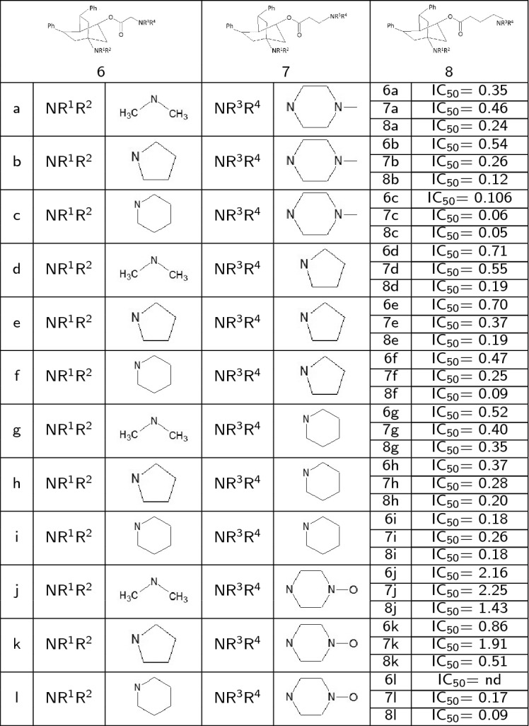
We employed a set of 4-aminobicyclo[2.2.2]octan-2-yl 4-aminobutanoates (Table 1) reported by Weis et al. [34] and evaluated compounds against the multiresistant K-1 strain of Plasmodium falciparum.
Table 1.
Compounds set
Codification of structures
The electrotopographic state index for atoms [17] was used to codify chemical structures. This index is defined by Eq. (1).
| 1 |
where is the calculated value of the atom i in the corresponding molecule and is the intrinsic value of the atom i calculated with Eq. (2).
| 2 |
where N is the principal quantum number of atom I, is the number of valence electrons in the molecular skeleton (-h) and is the number of electrons in the skeleton (). For each atom of the molecular skeleton, is the number of valence electrons, is the number of electrons in orbitals and h is the number of hydrogen atoms bonded.
represents the disturbance of the atoms of the environment, which is calculated by Eq. (3).
| 3 |
where the sum is over the difference of the intrinsic values of atom i with respect to each one of the other atoms in the molecule and is the Euclidean distance between the analyzed atoms, transforming the original topological index of Kier and Hall in topographic.
Graph reduction
The reduction of the chemical graph is carried out by the method described by Carrasco et al. [35], where the descriptor centers (DCs), rings of different orders (Rn), clusters of order 3 and 4 (C3 and C4, respectively), heteroatoms such as halogens, amino, etc. (X), and terminal groups such as methyl (), methylene () and methyne (M) are defined. Examples of these parameters are shown in Fig. 1. This graph reduction procedure, named CALEDE, is inspired by the procedure developed by Avindon et al. [36], where each DC is assigned the total value of , quantified as the sum of the value of of each atom that conforms to it.
Fig. 1.
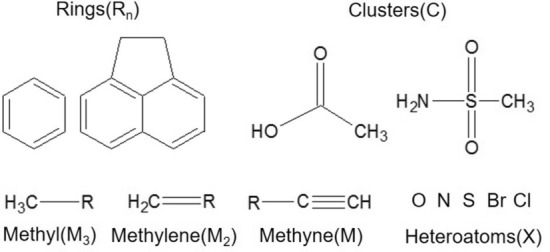
Examples of Descriptor Centers (DC) employed in the fragmentation of the chemical graphs
Definition of the maximum common property
The maximum common property (MCPhd) between two fully connected and complete (not hydrogen-depleted) and chemical graphs is defined as the maximum similarity in the chemical-physical properties represented by the index , which exists between subgraphs and of the molecular graphs and , respectively. Both and represent the link of at least two DCs that are at a Euclidean distance dE(, ) from their corresponding centers of mass from pairs of DCs.
To quantify the value of similarity between two compounds using the concept of the maximum common property (MCPhd), the calculation of the similarity of two compounds is assumed using the Tanimoto function or coefficient on the basis of the maximum common substructure called [15, 16]. The for two molecules A and B is defined as:
| 4 |
where is the number of links of A, is the number of links of B and is the number of links of the MCS of A and B. If the concept MCPhd is replaced in Eq. (4), it yields:
| 5 |
where is the number of heavy atoms of A, the number of heavy atoms of B and the smallest number of heavy atoms among the fragments with the highest MCPhd between A and B.
The proposed MCPhd algorithm
Figure 2 shows the algorithm used for the calculation of similarity. The algorithm uses the following parameters: ( and ) two compounds or molecules, (u) the similarity threshold, (f) the similarity coefficient and (i) the index used to quantify the similarity. First, we obtain the subgraphs ( and ) that have a maximum common property value quantified by the index based on the parameters and similarity coefficient. These subgraphs are obtained by performing the following steps:
The index (i) entered as a parameter is calculated for each atom in each G1 and G2 graph using the Chemical Development Kit (CDK) library [33]. Lines 1 and 2 of the algorithm are shown in Fig. 2.
The graphs ( and ) on DCs are reduced, and the total index value of each one is obtained. Lines 3 and 4 of the algorithm are shown in Fig. 2.
The similarity matrix between the DCs obtained from the graphs ( and ) is constructed using the similarity coefficient introduced as a parameter, along with the distance matrix between the DCs of each graph ( and ) using the Euclidean distance. Line 5 of the algorithm is shown in Fig. 2.
The DCs from each graph ( and ) that meet the condition that the similarity value must be higher than the similarity threshold (u), entered as a parameter, are selected. Line 5 of the algorithm is shown in Fig. 2.
Finally, using the list of DCs obtained in the previous step and the distance matrices of the DCs in graph and , a new distance matrix between pairs of DCs in each graph and is constructed using the Canberra distance coefficient [38], as shown in Fig. 3. Then for each pair of DCs selected, a list is created in which the pairs of DCs in the created matrix whose distance is less than or equal to 0.15 are stored. Finally, the largest lists is selected and from each one the subgraphs and are generated. Line 5 of the algorithm is shown in Fig. 2
Then, for a pair of subgraphs ( and ) obtained and the graphs ( and ), the values of the variables needed to quantify similarity are obtained using the similarity coefficient (u) for the discrete data entered as a parameter. Variable c is assigned the least number of heavy atoms belonging to the subgraphs ( and ), while variables a and b are assigned the number of heavy atoms belonging to each graph ( and ), respectively. Finally, these values are substituted in the similarity function to obtain the quantification of the similarity of the graphs (G1 and G2). Lines 6 to 16 of the algorithm are shown in Fig. 2. Furthermore, if there are several subgraphs and , the same operation is performed for each one and the pair of subgraphs and with the highest similarity value is selected.
Fig. 2.

MCPhd algorithm for similarity calculation
Fig. 3.

Distance matrix between pairs of similar DCs
The use of the algorithm is exemplified below using the molecules 6k and 6c present in the dataset as shown in Figs. 4 , 5, respectively. We use 5 parameters for its operation, where and are the molecular graphs 6k and 6c respectively, (i) is the index (), (u) is the similarity threshold, and (f) is the similarity function. For this example, we will use 0.95 and the modified Tanimoto coefficient () as the threshold and similarity function, respectively. Then, after assigning the parameters, the following steps are performed:
The index is calculated for each atom present in molecules 6k and 6c; these results are shown in Tables 2 and 3.
The 6k and 6c molecular graphs on DCs are reduced, and each is given the value of the total index. As shown in step A of Fig. 6, molecule 6k is reduced on the DCs (, , , , , , ), while molecule 6c is reduced on (, , , , , , ).
The similarity matrix between the DCs of each molecule 6k and 6c is constructed using the continuous Tanimoto coefficient (Tc) [37], together with the distance matrices between the DCs of each molecule (6k and 6c), as shown in step B of Fig. 6.
DCs are selected from each molecule (6k and 6c) that meet the condition that the similarity value is above the similarity threshold of 0.95. The DCs selected from molecules 6k and 6c are (, , , , and ) and (, , , , , and ), respectively, as shown in step C-a in Fig. 6. Furthermore, using the distance matrices of the graphs obtained in the previous step, for each pair of DCs, a list is constructed with the pairs of DCs that are at a Canberra distance less than or equal to 0.15, as shown in step C-b in Fig. 6.
From the lists of DC pairs obtained in the previous step, the following DCs are selected, namely, (, , and ) and (, , and ), corresponding to the lists (1, 3, 4 and 5) according to the larger size list with the same DCs in common.
Finally, the similarity value of the two molecules 6k and 6c is quantified using the modified Tanimoto coefficient (), where the value of is the lowest number of heavy bonds present between fragments and , while the values of and are obtained from the number of heavy atoms present in molecules 6k and 6c, respectively. With these values, it is possible to quantify the similarity between molecules 6k and 6c. In step E of Fig. 6, it can be seen that the number of heavy atoms of fragments and is 23 and 24, respectively, so the value of is 23, while the number of heavy atoms of molecules 6k and 6c is 36 and 37, respectively; that is, and . Therefore, the calculated value of similarity between molecules 6k and 6c is 0.46.
Fig. 4.
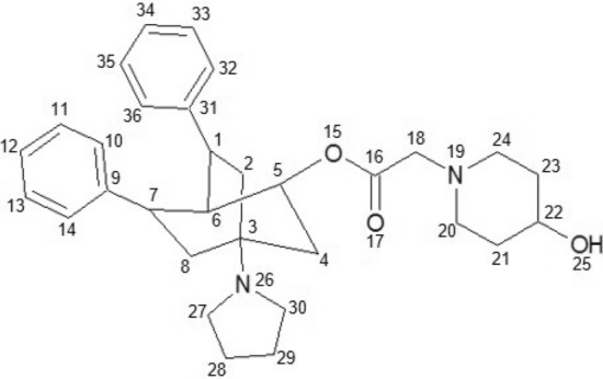
2D graph of the 6k molecule
Fig. 5.

2D graph of the 6c molecule
Table 2.
Result of the calculation for each atom of the molecule 6k
| Molecule 6k | |||||
|---|---|---|---|---|---|
| Atom | Number | Sstate3D | Atom | Number | Sstate3D |
| C | 1 | 0.27653 | N | 19 | − 1.4592 |
| C | 2 | 4.24474 | C | 20 | 3.38006 |
| C | 3 | − 2.11427 | C | 21 | 3.11542 |
| C | 4 | 4.25231 | C | 22 | − 0.12941 |
| C | 5 | 0.49396 | C | 23 | 3.09432 |
| C | 6 | 0.52371 | C | 24 | 3.32881 |
| C | 7 | 0.28273 | O | 25 | 4.22234 |
| C | 8 | 4.2063 | N | 26 | − 1.30847 |
| C | 9 | − 0.37931 | C | 27 | 3.52697 |
| C | 10 | 3.51969 | C | 28 | 2.9831 |
| C | 11 | 2.98731 | C | 29 | 3.01061 |
| C | 12 | 2.89649 | C | 30 | 3.54754 |
| C | 13 | 2.99502 | C | 31 | − 0.38433 |
| C | 14 | 3.5348 | C | 32 | 3.54001 |
| O | 15 | − 0.08644 | C | 33 | 2.99825 |
| C | 16 | − 0.10545 | C | 34 | 2.90069 |
| O | 17 | 5.5644 | C | 35 | 2.99544 |
| C | 18 | 3.75612 | C | 36 | 3.53921 |
Table 3.
Result of the calculation for each atom of the molecule 6c
| Molecule 6c | |||||
|---|---|---|---|---|---|
| Atom | Number | Sstate3D | Atom | Number | Sstate3D |
| C | 1 | 0.35527 | C | 20 | 3.314 |
| C | 2 | 4.17197 | C | 21 | 2.96595 |
| C | 3 | − 2.19195 | N | 22 | − 2.22668 |
| C | 4 | 4.25527 | C | 23 | 2.94306 |
| C | 5 | 0.37013 | C | 24 | 3.25612 |
| C | 6 | 0.50352 | C | 25 | 8.9881 |
| C | 7 | 0.21375 | N | 26 | − 1.46525 |
| C | 8 | 4.23211 | C | 27 | 3.52712 |
| C | 9 | − 0.24053 | C | 28 | 2.94719 |
| C | 10 | 3.50889 | C | 29 | 2.85191 |
| C | 11 | 3.00512 | C | 30 | 2.95634 |
| C | 12 | 2.94959 | C | 31 | 3.54763 |
| C | 13 | 3.09722 | C | 32 | − 0.13708 |
| C | 14 | 3.69435 | C | 33 | 3.3945 |
| O | 15 | − 0.48635 | C | 34 | 2.9161 |
| C | 16 | − 0.31876 | C | 35 | 2.85145 |
| O | 17 | 5.6053 | C | 36 | 2.96557 |
| C | 18 | 3.73854 | C | 37 | 3.52272 |
| N | 19 | − 1.66555 | |||
Fig. 6.

Example of applying the MCPhd algorithm to the 6k and 6c molecules belonging to the dataset
Small molecule subgraph MCS approach
The Small Molecule Subgraph Detector (SMSD) algorithm differs from previous MCS algorithms in that it uses a combination of several algorithms to find the common maximum subset and filters the results in a way that is chemically relevant because it incorporates chemical knowledge (coincidence of atom type with information sensitive and insensitive to the bond) while searching for molecular similarity. In addition, the algorithm calculates the maximum subgraph common between two molecules (A and B) by combining the power of the VFLibMCS, MCSPlus and CDKMCS algorithms. These algorithms are used on a case-by-case basis, depending on the molecules under consideration for the common maximum subgraph search [29]. This algorithm is implemented in the SMSD tool available free of charge on the official site of the European Institute of Bioinformatics.
General experimental procedure
The experiments were carried out as shown in Fig. 7, based on a test of 36 compounds with a 2D structure, which have been tested experimentally in the study conducted by Weis et al. in 2014 [34]. The 3D structure of each compound was obtained through the Corina online service [30]. The 2D structures were used to calculate the molecular similarity (all against all) with the SMSD, OBabel_FP2 and ISIDA algorithms, while the 3D structures were processed to calculate the index of each atom and to reduce their graphs on DCs in order to apply the MCPhd algorithm to calculate the molecular similarity (all against all), and to use the SHAFTS method. The similarity was calculated using the OBabel_FP2, SHAFTS and ISIDA methods through the web service CoSiAn (Combinatorial Similarity Analysis) [27] and ChemMapper [28]. Additional file 1 contains all necessary data/files to reproduce the results.
Fig. 7.

General experimental procedure
To quantify the value of similarity between different we defined the following coefficient based on continuous Tanimoto [37]:
| 6 |
where and are the value of A and B respectively.
Finally, the results obtained by all the algorithms were compared from different perspectives: (i) the statistical difference of the MCPhd results with respect to those obtained by the other methods; (ii) the ratio of the similarity values obtained by the different methods against the values obtained for ; (iii) the percentage of success for the different similarity methods to find structures with the same activity, similar to a screening process; (iv) the results of the different methods in relation to the concept of bioisosterism or the analogy between the physicochemical properties of the molecular fragments; (v) the computational cost.
The MCPhd algorithm was implemented using the JAVA language and CDK library, all test were executed on an Intel(R) Core(TM) i7-7500U PC with 16 GB of RAM.
Results and discussion
The molecular similarity methods compared in this work, SMSD OBabel_FP2, ISIDA, SHAFTS and MCPhd, use different approaches to quantify the similarity between two molecular graphs or molecules. Whereas SMSD employs graph isomorphism and no other properties associated to the molecular structure, OBabel_FP2 uses the similarity between hashed fingerprints that represent molecule substructures, ISIDA employs substructural molecular fragments, and SHAFTS adopts a hybrid similarity metric combined with molecular shape and colored chemistry groups for 3D molecular similarity calculation. The similarity calculated with MCPhd is based on the criterion of analogy or proximity between the physicochemical properties of the molecular fragments or subgraphs that are compared, expressing these properties as an value.
As we will show, this approach places MCPhd closer to the concepts of bioisosterism. Bioisosterism denote that two different molecules can afford similar biological responses if the structural features are accomplished by physicochemical property that is responsible in great measure of the biological response. This concept was coined by Friedman [39], extended by Burger [40] and recently used by Lassalas et al. [41] and Tahirova [42].
Using these different approaches, different similarity values were obtained. Table 4 shows the results of the comparison with the remaining 35 molecules of the sample, with compounds 8c and 7j used as target elements since they had the minimum and maximum values, respectively.
Table 4.
Molecular similarity values of the most active and inactive compounds with the rest of the dataset
| Molecule 8c | Target | Molecule 7j | |||||||||||
|---|---|---|---|---|---|---|---|---|---|---|---|---|---|
| OBabel_FP2 | SHAFTS | ISIDA | SMSD | MSChd | OBabel_FP2 | SHAFTS | ISIDA | SMSD | MSChd | ||||
| 1.00 | 1.00 | 1.00 | 1.00 | 1.00 | 1.00 | 8c | 0.05 | 0.82 | 0.78 | 0.88 | 0.61 | 0.42 | 0.02 |
| 0.90 | 1.00 | 0.97 | 0.67 | 0.97 | 0.97 | 7c | 0.06 | 0.92 | 0.82 | 0.90 | 0.83 | 0.43 | 0.03 |
| 0.91 | 1.00 | 0.97 | 0.95 | 0.77 | 0.74 | 8f | 0.09 | 0.88 | 0.80 | 0.90 | 0.64 | 0.60 | 0.04 |
| 0.92 | 1.00 | 0.90 | 0.90 | 0.70 | 0.74 | 8l | 0.09 | 0.89 | 0.77 | 0.97 | 0.61 | 0.35 | 0.04 |
| 0.77 | 0.87 | 0.90 | 0.65 | 0.77 | 0.68 | 6c | 0.106 | 0.74 | 0.73 | 0.81 | 0.60 | 0.29 | 0.05 |
| 0.98 | 0.79 | 1.00 | 0.97 | 0.75 | 0.55 | 8b | 0.12 | 0.80 | 0.88 | 0.88 | 0.62 | 0.33 | 0.06 |
| 0.82 | 0.84 | 0.88 | 0.67 | 0.71 | 0.37 | 7l | 0.17 | 1.00 | 0.83 | 1.00 | 0.92 | 0.62 | 0.08 |
| 0.72 | 0.87 | 0.87 | 0.67 | 0.53 | 0.35 | 6i | 0.18 | 0.79 | 0.73 | 0.83 | 0.61 | 0.29 | 0.09 |
| 0.92 | 1.00 | 0.97 | 0.93 | 0.75 | 0.35 | 8i | 0.18 | 0.89 | 0.78 | 0.90 | 0.62 | 0.43 | 0.09 |
| 0.89 | 0.76 | 0.97 | 0.87 | 0.46 | 0.33 | 8d | 0.19 | 0.86 | 0.91 | 0.90 | 0.68 | 0.64 | 0.09 |
| 0.90 | 0.93 | 0.97 | 0.92 | 0.56 | 0.33 | 8e | 0.19 | 0.87 | 0.77 | 0.90 | 0.65 | 0.42 | 0.09 |
| 0.91 | 0.90 | 0.97 | 0.90 | 0.55 | 0.31 | 8h | 0.20 | 0.88 | 0.74 | 0.90 | 0.64 | 0.33 | 0.09 |
| 0.97 | 0.77 | 1.00 | 0.92 | 0.50 | 0.25 | 8a | 0.24 | 0.79 | 0.87 | 0.88 | 0.65 | 0.69 | 0.12 |
| 0.82 | 0.89 | 0.95 | 0.70 | 0.74 | 0.24 | 7f | 0.25 | 0.99 | 0.77 | 0.92 | 0.87 | 0.51 | 0.12 |
| 0.88 | 0.82 | 0.97 | 0.65 | 0.69 | 0.23 | 7b | 0.26 | 0.90 | 0.76 | 0.90 | 0.85 | 0.33 | 0.13 |
| 0.82 | 1.00 | 0.95 | 0.69 | 0.73 | 0.23 | 7i | 0.26 | 1.00 | 0.82 | 0.92 | 0.89 | 0.44 | 0.13 |
| 0.82 | 1.00 | 0.95 | 0.67 | 0.53 | 0.21 | 7h | 0.28 | 0.99 | 0.83 | 0.92 | 0.92 | 0.34 | 0.14 |
| 0.73 | 0.71 | 0.90 | 0.59 | 0.46 | 0.16 | 6a | 0.35 | 0.69 | 0.87 | 0.81 | 0.64 | 0.64 | 0.18 |
| 0.91 | 0.74 | 0.97 | 0.85 | 0.45 | 0.16 | 8g | 0.35 | 0.88 | 0.88 | 0.90 | 0.67 | 0.71 | 0.18 |
| 0.71 | 0.82 | 0.87 | 0.61 | 0.37 | 0.15 | 6h | 0.37 | 0.78 | 0.75 | 0.83 | 0.63 | 0.43 | 0.19 |
| 0.80 | 0.73 | 0.95 | 0.68 | 0.54 | 0.15 | 7e | 0.37 | 0.97 | 0.94 | 0.92 | 0.89 | 0.35 | 0.19 |
| 0.82 | 0.74 | 0.95 | 0.62 | 0.43 | 0.14 | 7g | 0.40 | 1.00 | 0.84 | 0.92 | 0.97 | 0.73 | 0.21 |
| 0.87 | 0.71 | 0.97 | 0.61 | 0.61 | 0.12 | 7a | 0.46 | 0.88 | 0.91 | 0.90 | 0.89 | 0.71 | 0.24 |
| 0.71 | 0.90 | 0.87 | 0.68 | 0.54 | 0.12 | 6f | 0.47 | 0.78 | 0.75 | 0.83 | 0.63 | 0.46 | 0.25 |
| 0.91 | 0.91 | 0.90 | 0.88 | 0.54 | 0.11 | 8k | 0.51 | 0.88 | 0.72 | 0.97 | 0.62 | 0.35 | 0.27 |
| 0.70 | 0.71 | 0.87 | 0.60 | 0.38 | 0.11 | 6g | 0.52 | 0.77 | 0.88 | 0.83 | 0.66 | 0.66 | 0.28 |
| 0.76 | 0.76 | 0.90 | 0.63 | 0.56 | 0.10 | 6b | 0.54 | 0.73 | 0.83 | 0.81 | 0.61 | 0.31 | 0.29 |
| 0.80 | 0.75 | 0.95 | 0.64 | 0.44 | 0.10 | 7d | 0.55 | 0.97 | 0.87 | 0.92 | 0.94 | 0.74 | 0.30 |
| 0.70 | 0.86 | 0.87 | 0.62 | 0.38 | 0.08 | 6e | 0.70 | 0.77 | 0.77 | 0.83 | 0.64 | 0.33 | 0.40 |
| 0.68 | 0.74 | 0.87 | 0.61 | 0.39 | 0.08 | 6d | 0.71 | 0.75 | 0.91 | 0.83 | 0.68 | 0.68 | 0.40 |
| 0.71 | 0.70 | 0.81 | 0.63 | 0.36 | 0.06 | 6k | 0.86 | 0.78 | 0.85 | 0.90 | 0.61 | 0.37 | 0.50 |
| 0.92 | 0.75 | 0.90 | 0.83 | 0.42 | 0.04 | 8j | 1.43 | 0.89 | 0.85 | 0.97 | 0.65 | 0.65 | 0.83 |
| 0.82 | 0.70 | 0.88 | 0.65 | 0.52 | 0.03 | 7k | 1.91 | 0.99 | 0.99 | 1.00 | 0.95 | 0.50 | 0.97 |
| 0.71 | 0.70 | 0.81 | 0.59 | 0.38 | 0.02 | 6j | 2.16 | 0.78 | 0.86 | 0.90 | 0.64 | 0.64 | 1.00 |
| 0.82 | 0.78 | 0.88 | 0.61 | 0.42 | 0.02 | 7j | 2.25 | 1.00 | 1.00 | 1.00 | 1.00 | 1.00 | 1.00 |
To determine whether the results produced by the MCPhd methods are significantly different, a non-parametric statistical test is used for two independent Mann-Whitney samples [43] with a significance level of 5%. The results of the Mann-Whitney U statistic and p values (bilateral asymptotic significance) for the most active (8c) and least active (7j) compounds are shown in Table 5. As the p values for both compounds are below 0.05, it is concluded that the similarity values obtained by the MCPhd methods were significantly different from the other similarity methods.
Table 5.
Mann-Whitney test values between the MCPhd method with the remainder on the most active and inactive compounds in the dataset
| Methods | Molecule 8c | Molecule 7j | ||
|---|---|---|---|---|
| U of Mann-Whitney | p (Sig. Asint. Bilateral) | U of Mann-Whitney | p (Sig. Asint. Bilateral) | |
| MCPhd | ||||
| OBabel_FP | 131.50 | 0.00 | 33.00 | 0.00 |
| SHAFTS | 117.00 | 0.00 | 34.50 | 0.00 |
| ISIDA | 70.50 | 0.00 | 33.50 | 0.00 |
| SMSD | 245.50 | 0.00 | 98.00 | 0.00 |
Furthermore, it can be seen in Figs. 8, 9 for the most active compound (8c) and the least active compound (7j), respectively, that the results obtained by the similarity methods used showed a low correlation with the results achieved when applying the MCPhd method. Table 6 shows these results for all the active compounds in the dataset.
Fig. 8.

Correlation between the similarity of MCPhd and the rest of methods using the compound 8c as reference
Fig. 9.

Correlation between the similarity of MCPhd and the rest of methods using the compound 7j as reference
Table 6.
Correlation results between MCPhd and the rest of methods for the active compounds in the dataset
| Molecule | Correlation | ||||
|---|---|---|---|---|---|
| a | b | c | d | ||
| 8c | 0.05 | 0.57 | 0.68 | 0.55 | 0.43 |
| 7c | 0.06 | 0.50 | 0.69 | 0.47 | 0.43 |
| 8f | 0.09 | 0.44 | 0.62 | 0.24 | 0.40 |
| 8l | 0.09 | 0.45 | 0.71 | 0.33 | 0.53 |
| 6c | 0.106 | 0.45 | 0.50 | 0.40 | 0.44 |
| 8b | 0.12 | 0.49 | 0.05 | 0.36 | 0.35 |
| 7l | 0.17 | 0.44 | 0.42 | 0.38 | 0.47 |
| 6i | 0.18 | 0.39 | 0.46 | 0.37 | 0.45 |
| 8i | 0.18 | 0.48 | 0.82 | 0.50 | 0.48 |
| 8d | 0.19 | 0.26 | 0.00 | 0.20 | 0.30 |
| 8e | 0.19 | 0.31 | 0.42 | 0.14 | 0.28 |
| 8h | 0.20 | 0.38 | 0.41 | 0.30 | 0.40 |
| 8a | 0.24 | 0.42 | 0.19 | 0.26 | 0.40 |
| 7f | 0.25 | 0.34 | 0.33 | 0.15 | 0.41 |
| 7b | 0.26 | 0.50 | − 0.02 | 0.42 | 0.37 |
| 7i | 0.26 | 0.28 | 0.76 | 0.22 | 0.46 |
| 7h | 0.28 | 0.26 | 0.49 | 0.14 | 0.34 |
a-OBabel_FP2 vs MCPhd, b-SHAFTS vs MCPhd,
c-ISIDA vs MCPhd and d-SMSD vs MCPhd
As the maximum inhibitory concentration () is a measure of a compound’s efficacy in inhibiting biological or biochemical function, it is expected that compounds with near values of , are very similar and with far values of , the compounds will exhibit very low similarity. Under that hypothesis, the results were analyzed from another perspective. The similarity was calculated for the values of the variable of the most active compound (8c) and the less active compound (7j) against the rest of the dataset. The results are shown in the columns of Table 4.
Subsequently, the molecular similarities calculated by the different methods were compared with this new variable. As shown in Fig. 10, the similarity results obtained by the MCPhd method for the most active compound (8c) had a slope closer to that obtained with the similarity; furthermore, the results were better correlated obtained the MCPhd method the best Pearson correlation coefficient ( = 0.85) compared to the remaining methods as Fig. 11 shows.
Fig. 10.

Comparison of the molecular similarity between compound 8c and the rest of the dataset
Fig. 11.

Correlation between similarity methods and similarity values between compound 8c and the rest of the dataset
A similar behavior was observed in the results obtained for the less active compound (7j). The slope of MCPhd was closer to compared to the other methods (Fig. 12). The = 0.43 of MCPhd vs. was higher than the other similarity methods, with the exception of the SHAFTS method where = 0.55 (see Fig. 13).
Fig. 12.

Comparison of the molecular similarity between compound 7j and the rest of the dataset
Fig. 13.

Correlation between similarity methods and similarity values between compound 7j and the rest of the dataset
To generalize these results, the similarity obtained with all methods of the rest of the 17 compounds selected as active by Baptista [44] was correlated against . The results showed (Table 7) that overall the MCPhd method improved the correlation coefficient in 6% of the cases with respect to SHAFTS and 18% of the cases with respect to the remaining methods.
Table 7.
Results of correlation between similarity methods and TcIC50 similarity values for the active compounds in the dataset
| Molecule | Correlation | |||||
|---|---|---|---|---|---|---|
| a | b | c | d | e | ||
| 8c | 0.05 | 0.54 | 0.66 | 0.49 | 0.54 | 0.84 |
| 7c | 0.06 | 0.29 | 0.62 | 0.37 | 0.06 | 0.80 |
| 8f | 0.09 | 0.24 | 0.60 | 0.33 | 0.50 | 0.48 |
| 8l | 0.09 | 0.26 | 0.62 | 0.04 | 0.44 | 0.55 |
| 6c | 0.106 | − 0.11 | 0.10 | − 0.03 | − 0.13 | 0.64 |
| 8b | 0.12 | 0.50 | − 0.06 | 0.49 | 0.45 | 0.44 |
| 7l | 0.17 | 0.03 | 0.08 | − 0.07 | − 0.03 | 0.36 |
| 6i | 0.18 | − 0.37 | 0.11 | − 0.20 | − 0.16 | 0.25 |
| 8i | 0.18 | 0.26 | 0.64 | 0.33 | 0.46 | 0.56 |
| 8d | 0.19 | 0.22 | − 0.13 | 0.33 | 0.27 | − 0.15 |
| 8e | 0.19 | 0.23 | 0.29 | 0.33 | 0.38 | 0.13 |
| 8h | 0.20 | 0.24 | 0.25 | 0.33 | 0.35 | 0.12 |
| 8a | 0.24 | 0.50 | − 0.11 | 0.49 | 0.33 | − 0.07 |
| 7f | 0.25 | − 0.05 | 0.15 | 0.20 | 0.02 | 0.37 |
| 7b | 0.26 | 0.24 | − 0.09 | 0.37 | − 0.04 | 0.35 |
| 7i | 0.26 | − 0.03 | 0.60 | 0.20 | − 0.01 | 0.40 |
| 7h | 0.28 | − 0.05 | 0.57 | 0.20 | − 0.13 | − 0.02 |
a-OBabel_FP2 vs , b-SHAFTS vs , c-ISIDA vs ,
d-SMSD vs and e-MCPhd
To perform a more exhaustive study comparing the molecular similarity results obtained by all methods, the following steps were performed: (1) the similarity is calculated with all methods for all compounds (one against all); (2) the results up to or equal to the similarity thresholds (0.90, 0.80 and 0.70) are selected for each method; and (3) in each method, the threshold with the highest percentage of success in finding structures with the same activity is selected as the best threshold, and its results are compared.
As a result, a threshold of 0.90 was selected for the OBabel_FP2 method because 56% of the 137 pairs of structures found presented the same activity (active-active and inactive-inactive); for the remaining methods: SHAFTS, ISIDA, SMSD and MCPhd, thresholds of 0.80, 0.90, 0.90 and 0.70 were selected because they presented 53%, 55%, 65% and 67% of pairs of structures with the same activity respectively. Tables 8, 9, 10, 11 and 12 show the results that validate the selection.
Table 8.
Comparison of the observed and predicted by OBabel_FP2 for several similarity thresholds
| Threshold | Real-Predicted | Pairs | % | Predicted | Pairs | % |
|---|---|---|---|---|---|---|
| 0.90 | Active-active | 42 | 31 | Correct | 77 | 56 |
| Inactive-inactive | 35 | 26 | ||||
| Active-inactive | 32 | 23 | Incorrect | 60 | 44 | |
| Inactive-active | 28 | 20 | ||||
| Total | 137 | 100 | Total | 137 | 100 | |
| 0.80 | Active-active | 101 | 32 | Correct | 170 | 55 |
| Inactive-inactive | 69 | 22 | ||||
| Active-inactive | 65 | 21 | Incorrect | 141 | 45 | |
| Inactive-active | 76 | 24 | ||||
| Total | 311 | 100 | Total | 311 | 100 | |
| 0.70 | Active-active | 133 | 24 | Correct | 277 | 49 |
| Inactive-inactive | 144 | 26 | ||||
| Active-inactive | 86 | 15 | Incorrect | 287 | 51 | |
| Inactive-active | 201 | 36 | ||||
| Total | 564 | 100 | Total | 564 | 100 |
Pairs-Number of predicted pairs
Table 9.
Comparison of the observed and predicted by SHAFTS for several similarity thresholds
| Threshold | Real-predicted | Pairs | % | Predicted | Pairs | % |
|---|---|---|---|---|---|---|
| 0.90 | Active-active | 19 | 24 | Correct | 31 | 42 |
| Inactive-inactive | 13 | 18 | ||||
| Active-inactive | 18 | 24 | Incorrect | 43 | 58 | |
| Inactive-active | 25 | 34 | ||||
| Total | 74 | 100 | Total | 74 | 100 | |
| 0.80 | Active-active | 75 | 29 | Correct | 137 | 53 |
| Inactive-inactive | 62 | 24 | ||||
| Active-inactive | 43 | 17 | Incorrect | 120 | 47 | |
| Inactive-active | 77 | 30 | ||||
| Total | 257 | 100 | Total | 257 | 100 | |
| 0.70 | Active-active | 107 | 22 | Correct | 224 | 45 |
| Inactive-inactive | 117 | 24 | ||||
| Active-inactive | 76 | 15 | Incorrect | 271 | 55 | |
| Inactive-active | 195 | 39 | ||||
| Total | 495 | 100 | Total | 495 | 100 |
Pairs-Number of predicted pairs
Table 10.
Comparison of the observed and predicted by ISIDA for several similarity thresholds
| Threshold | Real-predicted | Pairs | % | Predicted | Pairs | % |
|---|---|---|---|---|---|---|
| 0.90 | Active-active | 94 | 32 | Correct | 165 | 55 |
| Inactive-inactive | 71 | 24 | ||||
| Active-inactive | 57 | 19 | Incorrect | 133 | 45 | |
| Inactive-active | 76 | 26 | ||||
| Total | 298 | 100 | Total | 298 | 100 | |
| 0.80 | Active-active | 136 | 23 | Correct | 289 | 49 |
| Inactive-inactive | 153 | 26 | ||||
| Active-inactive | 84 | 14 | Incorrect | 306 | 51 | |
| Inactive-active | 222 | 37 | ||||
| Total | 595 | 100 | Total | 595 | 100 | |
| 0.70 | Active-active | 136 | 23 | Correct | 289 | 49 |
| Inactive-inactive | 153 | 26 | ||||
| Active-inactive | 84 | 14 | Incorrect | 306 | 51 | |
| Inactive-active | 222 | 37 | ||||
| Total | 595 | 100 | Total | 595 | 100 |
Pairs-Number of predicted pairs
Table 11.
Comparison of the observed and predicted by SMSD for several similarity thresholds
| Threshold | Real-predicted | Pairs | % | Predicted | Pairs | % |
|---|---|---|---|---|---|---|
| 0.90 | Active-active | 39 | 34 | Correct | 75 | 65 |
| Inactive-inactive | 36 | 31 | ||||
| Active-inactive | 19 | 17 | Incorrect | 41 | 35 | |
| Inactive-active | 22 | 19 | ||||
| Total | 116 | 100 | Total | 116 | 100 | |
| 0.80 | Active-active | 52 | 28 | Correct | 106 | 57 |
| Inactive-inactive | 54 | 29 | ||||
| Active-inactive | 48 | 26 | Incorrect | 81 | 43 | |
| Inactive-active | 33 | 18 | ||||
| Total | 187 | 100 | Total | 187 | 100 | |
| 0.70 | Active-active | 63 | 30 | Correct | 121 | 57 |
| Inactive-inactive | 58 | 27 | ||||
| Active-inactive | 48 | 23 | Incorrect | 91 | 43 | |
| Inactive-active | 43 | 20 | ||||
| Total | 212 | 100 | Total | 212 | 100 |
Pairs-Number of predicted pairs
Table 12.
Comparison of the observed and predicted by MCPhd for several similarity thresholds
| Threshold | Real-predicted | Pairs | % | Predicted | Pairs | % |
|---|---|---|---|---|---|---|
| 0.90 | Active-active | 14 | 33 | Correct | 26 | 62 |
| Inactive-inactive | 12 | 29 | ||||
| Active-inactive | 8 | 19 | Incorrect | 16 | 38 | |
| Inactive-active | 8 | 19 | ||||
| Total | 42 | 100 | Total | 42 | 100 | |
| 0.80 | Active-active | 16 | 36 | Correct | 28 | 62 |
| Inactive-inactive | 12 | 27 | ||||
| Active-inactive | 9 | 20 | Incorrect | 17 | 38 | |
| Inactive-active | 8 | 18 | ||||
| Total | 45 | 100 | Total | 45 | 100 | |
| 0.70 | Active-active | 41 | 45 | Correct | 62 | 67 |
| Inactive-inactive | 23 | 25 | ||||
| Active-inactive | 15 | 16 | Incorrect | 30 | 33 | |
| Inactive-active | 15 | 16 | ||||
| Total | 92 | 100 | Total | 92 | 100 |
Pairs-Number of predicted pairs
If we analyze the results obtained with the best similarity thresholds in each method, we can infer that the percentage of structures found with the same activity (active-active and inactive-inactive) obtained with the MCPhd method (67%) was better than the results with the OBabel_FP2, SHAFTS, ISIDA and SMSD methods by 11%, 14%, 12% and 2% respectively. Analyzing only the active-active pairs, the increase was 14%, 16%, 13% and 11% (45% for MCPhd, 31% for Obabel_FP2, 29% for SHAFTS, 32% for ISIDA and 34% for SMSD). These results proved, once again, that the MCPhd method improved the similarity results obtained by the rest of similarity methods studied.
As another criterion, the 42 (OBabel_FP2), 75 (SHAFTS), 94 (ISIDA), 39 (SMSD) and 41 (MCPhd) pairs of compounds classified in the active-active category shown in Tables 8, 9, 10, 11 , 12 were compared for all methods, using the best thresholds. To do so, only the 17 active compounds in the dataset were consided and, relationship graphs were drawn for the compounds present in the active-active pairs for each method. Figure 14 shows this representation.
Fig. 14.
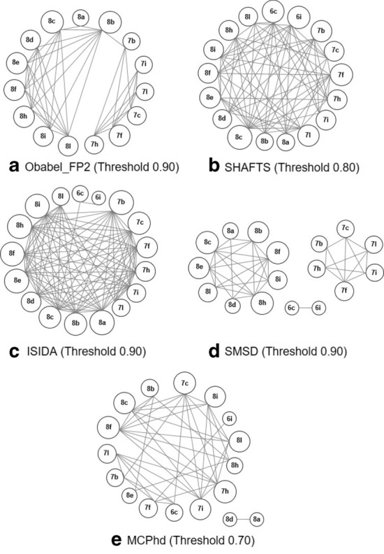
Relationship graph of active compounds with a molecular similarity higher than the selected threshold
If we observe the differences between the families of compounds 6, 7 and 8 (see Table 1), these differences were fundamentally due to the characteristics of the side chain. Moreover, the hybrid descriptors used in MCPhd have demonstrated [35, 45] their capability to distinguish between the same DC at different positions in a molecule. That allows MCPhd to find relationships/groups of compounds that show a higher functional relationship, and find similarities between compounds of different families. The rest of the compared methods did not show this capacity. As shown in Fig. 14, whereas MCPhd did not relate compounds 8d and 8a with the rest, suggesting that the electrostatic characteristics evidenced by the Electrotopographic State Index for Atoms was the source of the difference these two compounds. SMSD split this sample by grouping the three families separately, because it considers only structural features. SHAFTS considered that all compounds were related, and ISIDA identified similarity between 6c and 6i and the first of this pair with 8c.
This result implies that the MCPhd method allowed establishing similarity relations between compounds even from different families, making logical associations in contrast to the results of the other methods. The reason is that in addition to the structural information content provided by the electrotopographic state index for atoms, it includes the electrostatic information content.
As a last criterion, a runtime comparison was carried out for methods SMSD, SHAFTS and MCPhd. Figure 15 shows the box-plot representation of the computation time when calculating the similarity of each compound (reference structure) with the rest of the dataset. Moreover, the average runtime for SMSD was between 7688.2 and 8770.9 milliseconds, for SHAFTS was between 238.3 and 431.6 milliseconds. In contrast, the average calculation times for the MCPhd were between 18.6 and 35.6 milliseconds.
Fig. 15.

Calculation times
MCPhd uses a reduced graph, mapping smaller sized molecular graphs. In addition, the similarity calculated by the MCPhd method is based on the criterion of analogy or proximity between the physicochemical properties of the molecular fragments or subgroups that are compared by expressing these properties as a value of . On the other hand, SMSD and SHAFTS performs a more expensive mapping process for the compared molecular structures.
Conclusions
This work proposed a new approach that uses the 3D structure of molecules with physicochemical information to estimate the molecular similarity between chemical compounds. The method has been favorably compared with the standard SMSD, OBabel_FP2, ISIDA and SHAFTS methods and shows better performance in obtaining structures with the same activity using similarity cutoff values during the screening process. Furthermore, the proposal shows the ability to find similar compounds among different families. This strongly suggest the possibility of employing the MCPhd method for isosteric studies.
Finally, the proposal presented in this paper provides a promising method for extending this method to be used in the construction of QSAR models for molecular activity prediction.
Supplementary information
Additional file 1. rar-file containing all necessary data/files to reproduce the results presented in this work.
Acknowledgements
Not applicable.
Authors' contributions
Authors contributed equally to this work. All authors read and approved the final manuscript.
Funding
This work was supported in part by Project PID2019-109481GB-100 of the Spanish Ministry of Science and Innovation, by Project 1264182-F of the Andalusian Regional Government, by Project PP2019-Submod-1.2 of the Cordoba University and by Project AC25_2017 of the University of Informatics Sciences.
Availability of data and materials
All the data on which the conclusions of the work are based have been exhaustively presented in the manuscript. The algorithm implementation for free use, the dataset used in the paper, and other files needed to reproduce the results are included as supplementary material. The source code under GNU General Public License v3.0 can be downloaded from the GitHub repository at the following link: https://github.com/aantelo00/MCPhd.
Competing interests
The authors declare that they have no competing interests.
Footnotes
Publisher's Note
Springer Nature remains neutral with regard to jurisdictional claims in published maps and institutional affiliations.
Contributor Information
Aurelio Antelo-Collado, Email: aantelo@uci.cu.
Ramón Carrasco-Velar, Email: rcarrasco@uci.cu.
Nicolás García-Pedrajas, Email: npedrajas@uco.es.
Gonzalo Cerruela-García, Email: gcerruela@uco.es.
Supplementary information
Supplementary information accompanies this paper at 10.1186/s13321-020-00462-3.
References
- 1.Maggiora G, Vogt M, Stumpfe D, Bajorath J. Molecular similarity in medicinal chemistry. J Med Chem. 2013;57:3186–3204. doi: 10.1021/jm401411z. [DOI] [PubMed] [Google Scholar]
- 2.Kunimoto R, Vogt M, Bajorath J. Maximum common substructure-based Tversky index: an asymmetric hybrid similarity measure. J Comput Aided Mol Des. 2016;30:523–531. doi: 10.1007/s10822-016-9935-y. [DOI] [PubMed] [Google Scholar]
- 3.Vogt M, Stumpfe D, Geppert H, Bajorath J. Scaffold hopping using two-dimensional fingerprints: true potential, black magic, or a hopeless endeavor? guidelines for virtual screening. J Med Chem. 2010;12:5707–5715. doi: 10.1021/jm100492z. [DOI] [PubMed] [Google Scholar]
- 4.Gardiner EJ, Holliday JD, O’dowd C, Willett P. Effectiveness of 2D fingerprints for Scaffold hopping. Future Med Chem. 2011;3:405–414. doi: 10.4155/fmc.11.4. [DOI] [PubMed] [Google Scholar]
- 5.Good AC, Richards WG. Explicit calculation of 3D molecular similarity. Perspect Drug Discovery Des. 1998;9:321–338. [Google Scholar]
- 6.Rush TS, Grant JA, Mosyak L, Nicholls A. A shape-based 3-D Scaffold hopping method and its application to a bacterial protein-protein interaction. J Med Chem. 2005;48:1489–1495. doi: 10.1021/jm040163o. [DOI] [PubMed] [Google Scholar]
- 7.Moffat K, Gillet VJ, Whittle M, Bravi G, Leach AR. A comparison of field-based similarity searching methods: CatShape, FBSS, and ROCS. J Chem Inf Model. 2008;48:719–729. doi: 10.1021/ci700130j. [DOI] [PubMed] [Google Scholar]
- 8.Tresadern G, Bemporad D. Modeling approaches for ligand-based 3D similarity. Future Med Chem. 2010;2:1547–1561. doi: 10.4155/fmc.10.244. [DOI] [PubMed] [Google Scholar]
- 9.Hu Y, Stumpfe D, Bajorath J. Recent advances in scaffold hopping. J Med Chem. 2017;60:1238–1246. doi: 10.1021/acs.jmedchem.6b01437. [DOI] [PubMed] [Google Scholar]
- 10.Kenny PW, Sadowski J. Structure modification in chemical databases. Methods and Principles in Medicinal Chemistry. Wiley-Vch, Weinheim. 2005;23:271–285. [Google Scholar]
- 11.Hussain J, Rea C. Computationally efficient algorithm to identify matched molecular Pairs (Mmps) in large data sets. J Chem Inf Model. 2010;50:339–348. doi: 10.1021/ci900450m. [DOI] [PubMed] [Google Scholar]
- 12.Duesbury E, Holliday JD, Willett P. Maximum common subgraph isomorphism algorithms. Match Commun Math Comput Chem. 2017;77:213–232. [Google Scholar]
- 13.Cerruela García G, Luque Ruiz I, Gómez-Nieto MÁ. Step-by-Step calculation of all maximum common substructures through a constraint satisfaction based algorithm. J Chem Informat Comput Sci. 2004;44:30–41. doi: 10.1021/ci034167y. [DOI] [PubMed] [Google Scholar]
- 14.Cerruela García C, Palacios-Bejarano B, Luque Ruiz I, Gómez-Nieto MÁ. Comparison of representational spaces based on structural information in the development of QSAR models for benzylamino enaminone derivatives. SAR QSAR Environ Res. 2012;23(7–8):751–774. doi: 10.1080/1062936X.2012.719543. [DOI] [PubMed] [Google Scholar]
- 15.Maggiora GM, Shanmugasundaram V. Molecular similarity measures. Methods Mol Biol. 2004;275:1–50. doi: 10.1385/1-59259-802-1:001. [DOI] [PubMed] [Google Scholar]
- 16.Zhang B, Vogt M, Maggiora GM, Bajorath J. Design of chemical space networks using a tanimoto similarity variant based upon maximum common substructures. J Comput Aided Mol Des. 2015;29:937–950. doi: 10.1007/s10822-015-9872-1. [DOI] [PubMed] [Google Scholar]
- 17.Carrasco-Velar R (2007) Nuevos descriptores atómicos y moleculares para estudios de estructura-actividad: Aplicaciones. Editorial Universitaria, Ciudad de La Habana: 1–141. ISBN 978-959-16-0646-4
- 18.Kier LB, Hall LH. An electrotopological-State index for atoms in molecules. Pharm Res. 1990;7:801–807. doi: 10.1023/a:1015952613760. [DOI] [PubMed] [Google Scholar]
- 19.Nikolova N, Jaworska J. Approaches to measure chemical similarity-a review. QSAR Combinat Sci. 2003;22(9–10):1006–1026. [Google Scholar]
- 20.Raymond JW, Willett P. Similarity searching in databases of flexible 3D structures using smoothed bounded distance matrices. J Chem Inform Comput Sci. 2003;43(3):908–916. doi: 10.1021/ci034002p. [DOI] [PubMed] [Google Scholar]
- 21.Crippen GM, Havel TF. Distance geometry and molecular conformation. Taunton: Research Studies Press; 1988. [Google Scholar]
- 22.Hu J, Liu Z, Yu DJ, Zhang Y. LS-align: an atom-level, flexible ligand structural alignment algorithm for high-throughput virtual screening. Bioinformatics. 2018;34(13):2209–2218. doi: 10.1093/bioinformatics/bty081. [DOI] [PMC free article] [PubMed] [Google Scholar]
- 23.Liu X, Jiang H, Li H. SHAFTS: a hybrid approach for 3D molecular similarity calculation. 1. Method and assessment of virtual screening. J Chem Inform Model. 2011;51(9):2372–2385. doi: 10.1021/ci200060s. [DOI] [PubMed] [Google Scholar]
- 24.Quintus F, Sperandio O, Grynberg J, Petitjean M, Tuffery P. Ligand scaffold hopping combining 3D maximal substructure search and molecular similarity. BMC Bioinformatics. 2009;10(1):1–11. doi: 10.1186/1471-2105-10-245. [DOI] [PMC free article] [PubMed] [Google Scholar]
- 25.Kumar A, Zhang KY. Advances in the development of shape similarity methods and their application in drug discovery. Front Chem. 2018;6:315. doi: 10.3389/fchem.2018.00315. [DOI] [PMC free article] [PubMed] [Google Scholar]
- 26.O’Boyle NM, Banck M, James CA, Morley C, Vandermeersch T, Hutchison GR. Open babel: an open chemical toolbox. J Cheminform. 2011;3(1):33. doi: 10.1186/1758-2946-3-33. [DOI] [PMC free article] [PubMed] [Google Scholar]
- 27.CoSiAn (Combinatorial Similarity Analysis) Webserver (2020). http://cosian.cbs.cnrs.fr/from.html. Accessed 28 Jul 2020
- 28.Jiayu G, Chaoqian C, Xiaofeng L, Xin K, Hualiang J, Daqi G, Honglin L. ChemMapper: a Versatile web server for exploring pharmacology and chemical structure association based on molecular 3D similarity method. Bioinformatics. 2013;29:1827–1829. doi: 10.1093/bioinformatics/btt270. [DOI] [PubMed] [Google Scholar]
- 29.Rahman SA, Bashton M, Holliday GL, Schrader R, Thornton JM. Small molecule subgraph detector (SMSD) Toolkit. J Cheminform. 2009;1:12. doi: 10.1186/1758-2946-1-12. [DOI] [PMC free article] [PubMed] [Google Scholar]
- 30.Fast 3D Structure Generation with CORINA Classic (2020). https://www.mn-am.com/online_demos/corina_demo. Accessed 18 Feb 2020
- 31.Varnek A, Fourches D, Horvath D, Klimchuk O, Gaudin C, Vayer P, Marcou G. ISIDA-Platform for virtual screening based on fragment and pharmacophoric descriptors. Current Computer-Aided Drug Design. 2008;4(3):191. [Google Scholar]
- 32.Software Solutions and Services for Chemistry & Biology (2020). http://www.chemaxon.com. Accessed 30 Jul 2020
- 33.Willighagen EL, Mayfield JW, Alvarsson J, et al. The chemistry development kit (CDK)V2.0: atom typing, depiction, molecular formulas, and substructure searching. J Cheminf. 2017;9:33. doi: 10.1186/s13321-017-0220-4. [DOI] [PMC free article] [PubMed] [Google Scholar]
- 34.Weis R, Seebacher W, Brun R, Kaiser M, Sat R, Faist J. 4-Aminobicyclo[2.2.2]octan-2-yl 4-aminobutanoates with antiprotozoal activity. Monatsh Chem. 2013 [Google Scholar]
- 35.Carrasco R, Prieto JO, Antelo A, Padrón JA, Cerruela G, Maceo ÁL, Alcolea R, Silva LG. Hybrid reduced graph For SAR studies. SAR QSAR Environ Res. 2013;24:201–214. doi: 10.1080/1062936X.2013.764926. [DOI] [PubMed] [Google Scholar]
- 36.Avidon VV, Pomerantsev IA, Golender VE, Rozenblit AB. Structure-activity relationship oriented languages for chemical structure representation. J Chem Inf Comp Sci. 1982;22:207–214. [Google Scholar]
- 37.Steffen A, Kogej T, Tyrchan C, Engkvist O. Comparison of molecular fingerprint methods on the basis of biological profile data. J Chem Inform Model. 2009;49(2):338–347. doi: 10.1021/ci800326z. [DOI] [PubMed] [Google Scholar]
- 38.Lance GN, Williams WT. Computer programs for hierarchical polythetic classification ("similarity analysis") Comput J. 1966;9:60–64. [Google Scholar]
- 39.Friedman HL. Influence of isosteric replacements upon biological activity. Nat Acad Sci Nat Res Council. 1951;206:295. [Google Scholar]
- 40.Burger A (1991) Isosterism and bioisosterism in drug design in Progress in Drug Research. 37:287–371. 10.1007/978-3-0348-7139-6_7 [DOI] [PubMed]
- 41.Lassalas P, Oukoloff K, Makani V, James M, Tran V, Yao Y, Huang L, Vijayendran K, Monti L, Trojanowski JQ, Lee VM, Kozlowski MC, Smith AB, III, Brunden KR, Ballatore C. Evaluation of Oxetan-3-ol, Thietan-3-ol, and derivatives thereof as bioisosteres of the carboxylic acid functional group. ACS Med Chem. 2017;8:864–868. doi: 10.1021/acsmedchemlett.7b00212. [DOI] [PMC free article] [PubMed] [Google Scholar]
- 42.Tahirova N, Poivet E, Xu L, Peterlin Z, Zou DJ, Firestein SS. Bioisosterism reveals new structure-odor relationships. bioRxiv. 2019 [Google Scholar]
- 43.Mann HB, Whitney DR. On a test of whether one of two random variables is stochastically larger than the other. Ann Mathe Stat. 1947;18:50–60. [Google Scholar]
- 44.Baptista I, Camila Otero C, González S, Pertegás A, Galvez J, García R. Aplicación de la topología molecular al análisis de la actividad antimalárica de 4-Aminobiciclo [2.2.2]Octan-2 il 4-Aminobutanoatos y sus análogos etanoatos y propanoatos. Nereis. 2019;11:51–65. [Google Scholar]
- 45.Antelo A, Paneque JL, Hernández MC, Ramón Carrasco R. Molecular similarity using hybrid indices. Cuban J Med Inform. 2016;8:487–498. [Google Scholar]
Associated Data
This section collects any data citations, data availability statements, or supplementary materials included in this article.
Supplementary Materials
Additional file 1. rar-file containing all necessary data/files to reproduce the results presented in this work.
Data Availability Statement
All the data on which the conclusions of the work are based have been exhaustively presented in the manuscript. The algorithm implementation for free use, the dataset used in the paper, and other files needed to reproduce the results are included as supplementary material. The source code under GNU General Public License v3.0 can be downloaded from the GitHub repository at the following link: https://github.com/aantelo00/MCPhd.