Explainable and trustworthy artificial intelligence for correctable modeling in chemical sciences

The developed framework apportions model error to inputs, computes predictive guarantees, and enables model correctability.

Abstract

Data science has primarily focused on big data, but for many physics, chemistry, and engineering applications, data are often small, correlated and, thus, low dimensional, and sourced from both computations and experiments with various levels of noise. Typical statistics and machine learning methods do not work for these cases. Expert knowledge is essential, but a systematic framework for incorporating it into physics-based models under uncertainty is lacking. Here, we develop a mathematical and computational framework for probabilistic artificial intelligence (AI)–based predictive modeling combining data, expert knowledge, multiscale models, and information theory through uncertainty quantification and probabilistic graphical models (PGMs). We apply PGMs to chemistry specifically and develop predictive guarantees for PGMs generally. Our proposed framework, combining AI and uncertainty quantification, provides explainable results leading to correctable and, eventually, trustworthy models. The proposed framework is demonstrated on a microkinetic model of the oxygen reduction reaction.

INTRODUCTION

Models in the chemical and physical sciences have led to both new understanding and new discoveries (1) including new materials (2, 3). Physics-based models span orders of magnitude in length and time, ranging from quantum mechanics (4) to chemical plants (5), and naturally capture physics-based constraints (6–8). Combining models across scales, known as multiscale modeling (9), is necessary when chemical properties are determined at the quantum level, but most experiments and relevant applications exist at the macroscale, such as in heterogeneous catalysis. At the core of model development lies the question of accuracy of a physics-based model. Going beyond sensitivity analysis (10, 11), there has been growing interest in quantifying uncertainty, resulting from correlations in parameters (12, 13) along with other sources of error arising in predicting new materials (14). In addition to ensuring trustworthiness, error quantification can enable model correctability (15, 16). Still, uncertainty is an afterthought in actual physics-based model development. Currently, a model is first built deterministically without systematically accounting for the effect of both modeling errors and lack, or sparseness, of data.

Modeling uncertain data has experienced tremendous advances in data science (17–20); however, the corresponding models are empirical, can fail without guarantee, and can violate conservation laws and constraints. Current approaches for handling data based on physical laws and chemical theory are, in a sense, not truly probabilistic and require correlations and causal relationships to be known a priori. With the increasing size of chemistry datasets, it is almost impossible to apply traditional methods of model development to systems with many sources of interacting error. Global sensitivity techniques, such as Sobol indices, attribute model variance to model variables and their interaction (hereafter called “parametric uncertainty”) (21). However, there are few methods that work beyond first-order interactions or quantify the importance of missing physics or submodels rather than parameters (hereafter called “model uncertainty”) (22). Methods that do exist model missing physics as stochastic noise that has no structure (23, 24). Therefore, there is a need to develop methods that both attribute interaction error directly to model inputs and provide predictive guarantees and, by doing this, to make models correctable and eventually trustworthy for predictions and design tasks.

Here, we address these issues by incorporating error and uncertainty directly into the design of a model. First, we introduce the use of Bayesian networks (20), a class of probabilistic graphical models (PGMs) (25), common in probabilistic artificial intelligence (AI) (26), to integrate simultaneously and systematically physics- and chemistry-based models, data, and expert knowledge. This framework is termed C-PGM (chemistry-PGM). Second, we derive global uncertainty indices that quantify model uncertainty stemming from different physics submodels and datasets. This framework generates predictive “worst-case” guarantees for Bayesian networks while handling correlations and causations in heterogeneous data for both parametric and model uncertainties and is based on recent work in robust methods for quantifying probabilistic model uncertainty (27, 28). Our proposed framework, combining AI and uncertainty quantification (UQ), systematically apportions and quantifies uncertainty to create interpretable and correctable models; this is performed through assimilation of data and/or improvement of physical models to enable trustworthy AI for chemical sciences. We reduce the complexity of the nondeterministic polynomial time (NP)–hard problem of learning a PGM by leveraging expert knowledge of the underlying chemistry. We demonstrate this framework in the prediction of the optimal reaction rate and oxygen binding energy for the oxygen reduction reaction (ORR) using the volcano model. While UQ has been applied to deterministic volcano-based models in general (29), and the ORR model specifically (30), prior methods have been limited both by the physics model’s underlying structure and, importantly, the lack in interpretability of uncertainty in predictions in terms of modeling decisions and available data in different model components. We demonstrate that about half of the model uncertainty stems from density functional theory (DFT) uncertainty, comparable error from lack of sufficient number and quality of experimental data and from correlations in parameters (~20% each), and the remaining (~10%) from the solvation model. This analysis provides a blueprint for prioritizing model components toward correctability and improved trustworthiness by underscoring the need foremost of more accurate electronic structure calculations and secondary by better experiments. We illustrate model correctability with an example.

RESULTS

Physics model for the ORR and the deterministic volcano

Hydrogen fuel cells can nearly double the efficiency of internal combustion engines and leave behind almost no emissions, especially if environmentally low footprint H₂ is available (31). Furthermore, the hydrogen fuel cell is a mature technology that produces electricity via the hydrogen oxidation reaction at the anode and the ORR at the cathode (Fig. 1B); polymer electrolyte membrane fuel cells for this type of reaction are commercially available (32). Because of the high cost of platinum (Pt) catalyst and stability problems of other materials in an acidic electrolyte, recent focus has been on developing alkaline electrolytes. This technology, while extremely promising, results in slower reaction rates (by ~2 orders of magnitude compared to a Pt/acidic electrolyte) and thus bigger devices (33, 34). Overcoming slower rates with stable materials requires discovery of new, multicomponent catalysts, e.g., core-shell alloys.

Fig. 1. Fuel cell schematic with workflow and DFT data for estimating the optimal rate and properties of best materials.

(A) Key reaction steps (R1 to R4) in hydrogen fuel cells. R1, solvated O₂ forms adsorbed OOH*; R2, OOH* forms adsorbed surface oxygen O* and solvated H₂O; R3, O* forms adsorbed OH*; R4, H₂O forms and regenerates the free catalyst site. Asterisk (*) represents an unoccupied metal site or an adsorbed species; H⁺ and e⁻ refer to proton and electron, respectively. (B) Schematic of a hydrogen fuel cell. (C) Negative changes in Gibbs energies (−ΔG₁ and −ΔG₄) for reactions R1 (blue) and R4 (red) on the close packed (111/0001) surface of face-centered (fcc) and hexagonal close-packed (hcp) metals for the most stable sites of OOH*, OH*, and O* computed (specifically for this work) via DFT (circles) and linear regressions (lines). The optimal oxygen free energy $\mathrm{\Delta }{G}_{\mathrm{O}}^{*}$ is the intersection of the two lines. The min{ − ΔG₁, − ΔG₄}, indicated by the solid lines, determines the rate, estimated using Eq. 1. The optimal rate occurs at $\mathrm{\Delta }{G}_{\mathrm{O}}^{*}$. (D) Deterministic “human” workflow for obtaining the optimal formation energy of surface oxygen and the rate of the ORR.

The ORR depends on the formation of surface hydroperoxyl (OOH*), from molecular oxygen (O₂), and of water (H₂O), from surface hydroxide (OH*) (35). The complete mechanism (7, 36, 37) involves four electron steps (Fig. 1A) and is described in detail in section S1. Among these, reactions R1 and R4 are slow (7). Acceleration of the ORR then translates into finding materials that speed up the slower of the two reactions, R1 and R4. An approach to find new materials entails generation of an activity model (Fig. 1C) as a function of descriptor(s) that can be estimated quickly using DFT calculations (9). This is known as the deterministic volcano (Sabatier’s principle) and has been the key model for discovery of new materials.

Next, we discuss the human workflow in constructing the volcano curve. First, we use a physics equilibrium model to compute the rate r from the minimum free energy of reactions R1 and R4 (7, 38), such that

$$r=e^{\frac{\text{min}\{-\mathrm{\Delta }{G}_1,-\mathrm{\Delta }{G}_4\}}{k_{\mathrm{B}}T}}$$ (1)

where k_B is the Boltzmann constant and T is the temperature. Instead of Eq. 1, one could use a more elaborate model, such as a mean-field microkinetic (detailed reaction mechanism) or a kinetic Monte Carlo model, which is a more complex multiscale model. Such models impose conservation laws (mass conservation and catalyst site balance) and are selected on the basis of expert knowledge. The Gibbs free energy ΔG_i of the ith species is calculated from the electronic energy (E_DFT) and includes the zero-point energy, temperature effects, and an explicit solvation energy (E_solv) in water, as detailed in Methods. This calculation entails, again, physics-based models (statistical mechanics here) and expert knowledge, e.g., in selecting a solvation model and statistical mechanics models. See section S1 for an explanation of the equilibrium model and resulting formula in Eq. 1.

The free energies ΔG₁ and ΔG₄ are computed as linear combinations of the free energies of species, while accounting for stoichiometry (a constraint), and are regressed versus ΔG_O (the descriptor); see data in Fig. 1C. Typically, only two to three data points for coinage metals (Ag, Au, and Cu) on the right leg of the volcano are regressed, especially if experimental data (instead of DFT data) are used (data corresponding to dotted lines are not observed in most experiments). The intersection of the two lines (Fig. 1C) determines the maximum of the volcano curve and provides optimal material properties, i.e., the $\mathrm{\Delta }{G}_{\mathrm{O}}^{*}$; $\mathrm{\Delta }{G}_{\mathrm{O}}^{*}$ can then be matched to values of multicomponent materials to obtain materials closer to the tip of the volcano. This “human workflow” (Fig. 1D) provides a blueprint of the deterministic overall model that relies exclusively on expert knowledge in design and various physical submodels (called also components) for estimation of several key quantities.

Probabilistic AI for chemistry and the probabilistic volcano

Here, we develop a probabilistic AI-based workflow that augments the human workflow (in Fig. 1D) to create a probabilistic volcano. The mathematical tool we use to formulate the probabilistic volcano is the PGM. PGMs represent a learning process in terms of random variables, depicted as vertices of the graphs, which explicitly model their interdependence in terms of a graph. This interdependence stems from (i) one variable influencing others, called causality, depicted by arrows (directed edges); and (ii) correlations among variables, depicted by simple (undirected) edges between vertices (see below). PGMs are defined as the parameterized conditional probability distribution (CPD) and for Bayesian networks are defined such that

$$\begin{array}{c}P(X|\mathrm{\theta })={\displaystyle \prod _{i=1}^n}P(X_i|{\mathit{Pa}}_{X_i},{\mathrm{\theta }}_{X_i|P{a}_{X_i}}) \text{with} \text{CPD}:P(X_i|{\mathit{Pa}}_{X_i},\\ {\mathrm{\theta }}_{X_i|P{a}_{X_i}}),i=1,\dots ,n\end{array}$$ (2)

Pa_Xi = {X_i1…, X_im} ⊂ {X₁…, X_n} denotes the parents of the random variable X_i, and θ = {θ_{Xi ∣ PaXi}}ⁿ_{i = 1} are the parameters of each CPD, P(X_i ∣ Pa_Xi, θ_XiPaXi). Uppercase “P” indicates a stochastic model or submodel. A key concept in PGMs is that the random variables are conditionally independent. This concept is central to constructing complex probability models with many parameters and variables, enabling distributed probability computations by “divide and conquer” using graph-theoretic model representations. By combining the conditional probabilities in Eq. 2, we find the joint probability distribution of all random variables X. A detailed formalism for the construction of the PGM is given in section S4.

Structure learning of graphical models is, in general, an NP-hard problem (39, 40) if one considers the combinatorial nature in connecting a large number of vertices. We overcome this challenge by constraining the directed acyclic graph (DAG) (41), representing the probabilistic ORR volcano (Fig. 2A), using domain knowledge that includes multiscale, multiphysics models discussed above, expert knowledge, and heterogeneous data (experimental and DFT) along with their statistical analysis.

Fig. 2. Construction of the PGM.

(A) PGM (Eq. 3) for the ORR that combines heterogeneous data, expert knowledge, and physical models; causal relationships are depicted by arrows. The PGM P is a Gaussian Bayesian network where the CPDs are selected to be Gaussians [solid lines as histogram approximations in (B) to (E)]. The PGM is built as follows: We construct ΔG_{O (DFT)} as a random variable from the quantum data for the oxygen binding energy; we include statistical correlations between ΔG_{O (DFT)} and ΔG₁/ ΔG₄ (Fig. 1C) as a random error in correlation (B); (C to E) we model different kinds of errors in the ΔG’s, given expert knowledge; we include these random variables into the PGM and build the causal relationships (directed edges/arrows) between the corresponding random variables (ΔG’s); we obtain a prediction for the optimal oxygen binding energy ($\mathrm{\Delta }{G}_{\mathrm{O}}^{*}$) and optimal reaction rate (r*) using physical modeling, e.g., $\mathrm{\Delta }{G}_{\mathrm{O}}^{*}$ corresponds to the value where ΔG₁ and ΔG₄ are equal in the deterministic case. This entire figure captures the (probabilistic) “AI workflow” that augments the human workflow.

First, statistical analysis of data finds hidden correlations or lack thereof between variables and is also central to building the PGM. In this example, statistical analysis of the computed formation free energy data of O*, OOH*, and OH* indicates correlations among data, i.e., connections between vertices (Fig. 2A). Specifically, ΔG_OOH and ΔG_OH are correlated with ΔG_O. The correlation coefficients of ΔG_O with −ΔG₁ and −ΔG₄ are −0.95 and 0.91, respectively; see section S4 for notes on statistical independent tests used. Reaction free energies ΔG₁ and ΔG₄ are linear combinations of ΔG_OOH and ΔG_OH, respectively; we use the reaction free energies as dependent vertices, as the reaction rate depends directly on ΔG₁ and ΔG₄. Subsequently, we choose ΔG_O as the independent node (descriptor) because, of all the surface intermediates, it has the fewest degrees of freedom (and therefore local minima) on any given potential energy surface for faster quantum calculations. The selection of the descriptor, which is another example of expert knowledge in our C-PGM, establishes causal relationship (direction of influence) represented by directed edges from ΔG_O to ΔG₁ and ΔG₄. Expert knowledge is also leveraged to assign relevant errors (ω) to vertices and directed edges. Figure 2A (colored circles) depicts the multiple uncertainties (random variables) ω modeled in each CPD of the PGM and how these (causally) influence the uncertainty of each vertex. All these causal relationships are modeled by a DAG in Fig. 2A and the Bayesian network in Eq. 3. Causality simplifies the construction and UQ analysis of the PGM. Last, the lack of an edge between ΔG₁ and ΔG₄ (Fig. 2A) is found from conditional independence tests on the DFT data. By eliminating graph edges of uncorrelated parts of the graph, the constrained DAG is profoundly simpler. A complete, step-by-step discussion of the structure learning of the ORR C-PGM is included in section S4.1.

The C-PGM structure contains information from expert knowledge, causalities, physics (physical models, conservation laws, and other constraints), correlations of data, parameters, and hierarchical priors (priors of a prior) in model learning (13, 25). The physical meaning and estimation of these uncertainties are discussed below. Overall, the model for the ORR C-PGM becomes

$$\begin{array}{c}{\prod }_{i=\{1,4\}}p(\mathrm{\Delta }{G}_i|\mathrm{\Delta }{G}_{\mathrm{O} (\text{DFT}),}{\mathrm{\omega }}_{\mathit{ci}},{\mathrm{\omega }}_{\mathit{si}},{\mathrm{\omega }}_{\mathit{ei}},{\mathrm{\omega }}_{\mathit{di}}){\prod }_{j=\{c,s,e,d\}}p({\mathrm{\omega }}_{\mathit{ji}})\\ p(\mathrm{\Delta }{G}_{\mathrm{O} (\text{DFT})}|{\mathrm{\omega }}_{s\mathrm{O}},{\mathrm{\omega }}_{e\mathrm{O}},{\mathrm{\omega }}_{d\mathrm{O},}\mathrm{\Delta }{G}_{\mathrm{O}}){\prod }_{k=\{s,e,d\}}p({\mathrm{\omega }}_{k\mathrm{O}})\end{array}$$ (3)

where ΔG_{O (DFT)} indicates a calculated value from DFT and all other ΔG values represent the “true value” given errors. Lowercase “p” indicates probability densities that are assumed here to be Gaussian, thus rendering the C-PGM (Eq. 3) into a Gaussian Bayesian network (25). Note that this PGM is used as part of an optimization scheme where ΔG_{O (DFT)} is formulated as a random variable given any value of the true ΔG_O and distribution of errors for ΔG_O. Leveraging the human-based (deterministic) workflow in Fig. 1D, the ORR is modeled as a stochastic optimization problem such that

$$\mathrm{\Delta }{G}_{\mathrm{O}}^{*}≔{\text{argmax}}_{\mathrm{\Delta }{G}_{\mathrm{O}}}[E_P[\text{min}\{-\mathrm{\Delta }{G}_1,-\mathrm{\Delta }{G}_4\}|\mathrm{\Delta }{G}_{\mathrm{O}}]]$$ (4)

where $\mathrm{\Delta }{G}_{\mathrm{O}}^{*}$ corresponds to the optimal oxygen binding energy that maximizes the reaction rate r*. It is convenient to compute k_BT ln (r*),

$$k_{\mathrm{B}}T\text{ln}(r^{*})≔{\text{max}}_{\mathrm{\Delta }{G}_{\mathrm{O}}}[E_P[\text{min}\{-\mathrm{\Delta }{G}_1,-\mathrm{\Delta }{G}_4\}|\mathrm{\Delta }{G}_{\mathrm{O}}]]$$ (5)

For the rest of this paper, $\mathrm{\Delta }{G}_{\mathrm{O}}^{*}$ and k_BT ln (r*) are considered as the QoIs (quantities of interest) that need to be optimized.

Model uncertainty, guarantees, nonparametric sensitivity, and contributions to model error for interacting variables

Model uncertainty arises from multiple sources, such as use of sparse data in Fig. 1C, hidden correlations between vertices in the graph, simplified statistics models (linear regression between free energies in Fig. 1C and Gaussian approximations of errors; Fig. 2, B to E), and uncertainty in different model components and variables. These include errors in experimental data (ω_e), DFT data (ω_d), solvation energies (ω_s), and regressions (correlations) used to determine the optimum $\mathrm{\Delta }{G}_{\mathrm{O}}^{*}$ (ω_c); correlation error is accentuated by the small data available especially on the right leg of the volcano. Experimental errors (ω_e) in ΔG_O and ΔG_OH can be found by repeated measurements in the same laboratory and between different laboratories. Repeated calorimetry and temperature-programmed desorption measurements for the dissociative adsorption enthalpy of O₂ in the same and different labs provide a distribution of errors for ΔG_O. The distribution of DFT errors (ω_d) is computed by comparing experimental and calculated (DFT) data across various metals. The mean value and SD of errors are provided in table S1 along with a detailed description of how errors were calculated in Methods and section S3. In Fig. 2A, the “parent vertex” is determined by the direction of the arrow such that ω_e1 is a parent of ΔG₁ (the child). These additional uncertainties from multiple sources are shown in Fig. 2 (B to E) and are combined to build the PGM model P.

When building the C-PGM model P, “model uncertainties” arise from the sparsity and quality of the available data in different components of the model, the accuracy of the physics-based submodels, and the knowledge regarding the probability distribution of the errors (Fig. 2, B to E). Consequently, the mean value of min{ − ΔG₁, − ΔG₄} with respect to P is itself uncertain since the probabilistic model P is uncertain. For this reason, we consider P as a baseline C-PGM model, i.e., a reasonable but inexact “compromise.” Here, we take P to be a Gaussian Bayesian network (see Fig. 2, B to E), where the error probability distribution function for each component of the model is approximated as a normal distribution and is built using the nominal datasets and submodels discussed above. We isolate model uncertainty in each component (CPD) of the entire model (Eq. 3), in contrast to the more standard parametric (aleatoric) uncertainty already included in the stochasticity of P itself. We mathematically represent model uncertainty through alternative (to P) models Q that include the “true” unknown model Q*. As examples, models Q can differ from P by (i) replacing one or more CPDs in Eq. 3 by more accurate, possibly non-Gaussian CPDs that represent better the data in Fig. 2 (B to E), (ii) more accurate multiscale physics models, and (iii) larger and more accurate datasets. Quantifying the impact of model uncertainties on predicting the QoI using P, instead of better alternative models Q, is discussed next. Overall, developing the mathematical tools to enable identification of the components of a PGM that need improvement is critical to correct the baseline model P with minimal resources.

Each model Q is associated with its own model misspecification parameter η that quantifies how far an alternative model Q is from the baseline model P via the Kullback–Leibler (KL) divergence of Q to P, R(Q‖P). We use the KL divergence due to its chain rule properties that allow us to isolate the impact of individual model uncertainties of CPDs in Eq. 2 on the QoIs in Fig. 2, see sections S6 and S7. To isolate and rank the impact of each individual CPD model misspecification (η_l), we consider the set of all PGMs Q that are identical to the entire PGM P except at the lth component CPD (for dependence on the lth parents) and less than η_l in KL divergence from the baseline CPD P(X_l ∣ Pa_Xl) while maintaining the same parents Pa_Xl. We refer to this family, denoted by D^η_l, as the “ambiguity set” for the lth CPD of the PGM P (see section S6 for its mathematical definition). Given the set of PGM’s D^η_l, we develop model uncertainty guarantees $J_l^{\pm }(\text{QoI},P;{\mathrm{\eta }}_l)$ for the QoI in Eq. 6 as the two worst-case scenarios for all possible models Q in D^η_l with respect to the baseline P

$$J_l^{\pm }(\text{QoI},P;{\mathrm{\eta }}_l)=({\text{max}/\text{min})}_{Q\in D^{{\mathrm{\eta }}_l}}[E_Q(\text{QoI})-E_P(\text{QoI})]$$ (6)

For a given η_l, the model uncertainty guarantees to describe the maximum (worst case) expected bias when only one part of the model in the PGM, P(X_l ∣ Pa_Xl), is perturbed within η_l; therefore, they measure the impact of model uncertainty in any component (CPD) of the PGM on the QoI. Since η_l are not necessarily small, the method is also nonperturbative, i.e., it is suitable for both small and large model perturbations.

Equation 6 can be also viewed as a nonparametric model sensitivity analysis for PGMs since it involves an infinite dimensional family of model perturbations D^η_l of the baseline model P. This family can consider the sparsity of data by addition of new or higher-quality data, e.g., higher-level DFT data, alternative densities to the Gaussians in Fig. 2 (B to E), e.g., richer parametric families or kernel-based CPDs, or more accurate submodels. All these are large, nonparametric perturbations to the baseline P model. For these reasons, Eq. 7 allows one to interpret, reevaluate, and improve the baseline model by comparing the contributions of each CPD to the overall uncertainty of the QoIs through the (model uncertainty) ranking index

$$\begin{array}{c}\text{Ranking Index}=\text{Relative contribution to total model}\\ \text{uncertainty}=\frac{J_l^{\pm }(\text{QoI},P;{\mathrm{\eta }}_l)}{{\Sigma }_j{J}_j^{\pm }(\text{QoI},P;{\mathrm{\eta }}_j)}\end{array}$$ (7)

For more details, see theorem 1 in section S6 where we show that for Gaussian Bayesian networks, the ratios in Eq. 7 are computable.

We can use two strategies regarding η_l. First, η_l can by tuned “by hand” to explore how levels of uncertainty in each component of the model, P(X_l ∣ Pa_Xl), affect the QoIs. This approach is termed a stress test in analogy to finance where in the absence of sufficient data, models are subjected to various plausible or extreme scenarios. Second, instead of treating η_l as a constant, we can estimate η_l as the “distance” between available data from the unknown real model and our baseline PGM P; we refer to such η_l’s as data based, in contrast to stress tests (see section S8). For example, the data can be represented by a histogram or a kernel density estimator (KDE) approximation (42). In this sense, the contribution to model uncertainty from any error source is both a function of its variance and how far away the error is from the baseline, e.g., the Gaussian CPDs in Fig. 2 (B to E).

Given the error distributions and their Gaussian representation in PGM model P, the expected value of min{ − ΔG₁, − ΔG₄} ∣ ΔG_O (black curve) in Fig. 3A is obtained. The color bar in Fig. 3A indicates how likely a reaction rate occurs with given ΔG_O for model P (aleatoric uncertainty). The gray dashed lines in Fig. 3A correspond to the two extreme scenarios (derived in section S5) for all possible models Q by considering uncertainty in all components. We highlight in Fig. 3B the expected value (black line) and the extremes (gray dashed lines) when only the DFT error in ΔG₄ is considered. All η values here are data based and determine what models Q are considered in construction of the bounds; only PGMs that have a KL divergence that is less than or equal to η from the baseline are considered. The red, orange, and green lines indicate potential QoIs that can be computed; here, we focus on the uncertainty in the rate (y axis; difference between red lines) and the variability of optimal oxygen binding energy (x axis; difference between orange lines) as a proxy of materials selection; see section S7 for more details.

Fig. 3. Parametric and model uncertainty.

(A) Parametric versus model uncertainty: Contour plot of the probability distribution of min{ − ΔG₁, − ΔG₄} as a function of ΔG_O; the black curve is the mean (expected) value ${\mathbb{E}}_P[\text{min}\{-\mathrm{\Delta }{G}_1,-\mathrm{\Delta }{G}_4\}|\mathrm{\Delta }{G}_{\mathrm{O}}]$ for the baseline ORR PGM P in Fig. 2. The gray dashed lines are the extreme bounds (guarantees) with combined model uncertainty, and the color indicates likelihood; see section S5 for more details. (B) Model uncertainty guarantees given by the predictive uncertainty (model sensitivity indices) (gray dashed lines) for the QoI min{ − ΔG₁, − ΔG₄} ∣ ΔG_O when only the uncertainty of DFT in ΔG₄ is considered.

Using the model uncertainty guarantees (Eq. 6), we quantify the uncertainty and its impact on model predictions beyond the established parametric uncertainty; again, all η_l’s are data based. By sourcing the impact of each submodel and/or data, Eq. 7 reveals what data, measurement, and computation should be improved. The error in the optimal reaction rate (Fig. 4A) stems from a nearly equal contribution of submodels, specifically by solvation (30%), experiment (18%), DFT (33%), and parameter correlation (18%). The uncertainty in the optimal oxygen free energy variability (Fig. 4B), i.e., the materials prediction, stems from solvation (6%), experiment (8%), DFT (48%), and parameter correlation (37%). Different QoIs are influenced to a different degree by different submodels. In both QoIs, the DFT error stands as the most influential. The correlation between O*, OOH*, and OH* is the next most important component regarding materials prediction, whereas solvation is the second ranked component regarding reaction rate. Such predictions are nonintuitive. While previous work found that parametric-based microscale uncertainties can be dampened in multiscale models (43), the results of this work will generalize to any models where fine-scale simulations (such as DFT) are sparse or the macroscale QoIs can be made proportional to the microscale properties. In the next section, we show that Eq. 6 and the resulting Fig. 4 can also be deployed to improve the baseline (purely Gaussian) model P.

Fig. 4. Ranking indices for optimal rate and optimal oxygen binding energy in each ORR PGM submodel.

Rankings for the model uncertainties in k_BT ln (r*) (A) and $\mathrm{\Delta }{G}_{\mathrm{O}}^{*}$ variability (B). See section S7 for more details.

Model correctability enabled by model UQ

Model uncertainty due to any submodel or dataset, quantified by η_l and Eq. 6, can be reduced by picking a better submodel or dataset than the original baseline model P_l. Obviously, those CPDs that exhibit larger relative predictive uncertainty in Eq. 6 should be prioritized and corrected. In our case study, reducing the DFT error requires to further develop DFT functional and methods, a long-standing pursue not addressed here. Here, we illustrate how to carry out such model correctability through an example that is feasible to do. Specifically, we consider the model consisting of the data used to construct the volcano and its statistical representation as this is the second most influential parameter in materials prediction. We performed additional DFT calculations on core-shell bimetallics to create an expanded dataset compared to that in Fig. 1C (see Fig. 5A). By doing this, we compute the model sensitivity indices $J_l^{\pm }$ for the new model using theorem 1 and equation S58. More details and derivations are included in Methods.

Fig. 5. Correctability of the submodel determining the volcano using DFT data.

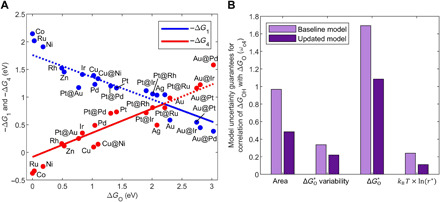
(A) Volcano curve with additional bimetallic data where M1@M2 indicates a shell of metal 1 on metal 2. (B) Uncertainty bounds when accounting for correlation error of the area of uncertainty region, $\mathrm{\Delta }{G}_{\mathrm{O}}^{*}$ variability, $\mathrm{\Delta }{G}_{\mathrm{O}}^{*}$, and k_BT ln (r*) for both the baseline model (light purple bars) and model with bimetallic data included (dark purple bars).

Figure 5B shows the reduction of model uncertainty guarantees, defined as Eq. 6, which are due to the variance of error and the estimated model misspecification parameter in the correlation between DFT-calculated values of ΔG₄ and ΔG_O, when more data (bimetallics) are added. With bimetallic data included, the correlation coefficients of ΔG_O with −ΔG₁ and −ΔG₄ are −0.95 and 0.95, respectively. The uncertainty is reduced both due to improved correlation and reduced SE in the regression coefficients as a result of more data.

DISCUSSION

Here, we introduce PGM for chemistry to embed uncertainty into the design of a model. The approach provides a blueprint to systematically integrate desperate components of a model ranging from heterogeneous data (experimental and DFT) to expert knowledge to physics/chemistry models and constraints to correlations among data and causality between variables. Instead of a deterministic model, a probabilistic ensemble of models is created. Furthermore, the model uncertainty and sensitivity indices derived herein provide guarantees on model prediction to systematically identify the most influential model components causing predictive uncertainty and ultimately ensure trustworthiness of predictions. Overall, our proposed mathematical framework combines probabilistic AI and UQ to provide explainable results, leading to correctable and, eventually, trustworthy models. We illustrate this framework for a volcano-kinetic model for the ORR. We propagate both parametric and model uncertainty from several, small sets of input data to model predictions. We establish model error bounds on the ORR volcano to assess maximum and minimum rates given the binding energy of atomic oxygen as the primary descriptor. We assess the impact of these errors via model sensitivity indices, which quantify the percent error from uncertainty contributed by each variable to the predicted maximum ORR rate and the oxygen binding energy corresponding to that rate. The greatest contribution to errors (ordered from greatest to least) in the PGM-based ORR volcano in predicting materials arises from error in DFT calculations and correlations of OOH* and OH* binding energies with O* binding energies. Different from the materials, the reaction rates depend mainly on errors associated with DFT and solvation, yet experimental error and correlations are relatively large as well, i.e., a more equidistribution of error is observed and improved accuracy of all components is needed to size electrochemical devices. Improving the accuracy of DFT method and the quality and quantity of data can pave the way for more accurate models for finding new catalysts.

METHODS

DFT calculations

We study adsorption on the close-packed (111 and 0001) transition metal surfaces. We select the lowest energy site of O* and OH* for comparison with experiments to determine errors, which are summarized in table S1. We build the correlations for bimetallics from the lowest energy sites on the (111) and (0001) surfaces of the face-centered (fcc) and hexagonal close-packed (hcp) metals, respectively.

Vacuum phase DFT setup

We calculated binding energies and vibrational frequencies using the Vienna ab initio Simulation Package version 5.4 with the projector-augmented wave method (44). We use the Revised Perdew-Burke-Ernzerhof (RPBE) density functional (45) with D3 dispersion corrections (46). Simulation methods include use of spin-polarized calculations for gas-phase species and ferromagnetic metals, a 3 × 3 × 1 Monkhorst-Pack k-point sampling grid (47) for all slab calculations, and a 400-eV plane wave cutoff. Electronic energy convergence was set to 10⁻⁴ eV for the energy minimization step and 10⁻⁶ eV for frequency calculations.

For calculations of gas-phase species, the supercell size was 10 × 10 × 10 Å. A Brillouin zone was sampled at the gamma point; a 0.005 eV/Å force cutoff was used in geometry optimizations. For slab calculations, the force cutoff was set to 0.02 eV/Å with 20 Å of vacuum space. Adsorbate energies were calculated for OOH*, OH*, and O* on the most stable close-packed surface for fcc and hcp metals. The periodic cell consisted of four layers with 16 metal atoms in each layer; the bottom two layers were fixed at their bulk values, determined using a 15 × 15 × 15 k-point grid with the tetrahedron method and Blöchl corrections. Bulk metal lattice constants were pre-optimized with DFT using the Birch-Murnaghan equation of state (48). Zero-point energies are calculated for each adsorbate-surface combination and for all gas species. All input files were created using the Atomic Simulation Environment (49).

Solvation phase DFT setup

We emulate explicit solvation calculations from previous work (38) except that, here, we vary the number of water layers. Two to five layers of water were placed above a Pt(111) surface in a honeycomb pattern to simulate the aqueous phase above the surface. The double layer of water molecules was found to adequately capture water binding energies on Pt(111) and H bonds at the surface (50). We determined solvation energies for O* by placing it in an fcc hollow site on the water-covered surface. For OH* and OOH*, solvation energies were determined by replacing a water molecule on the surface with the respective species to determine solvation energies. Other than the choice of functional, the DFT setup was identical to that in the vacuum except that nine Pt atoms were included in each layer to accommodate the honeycomb water structure, the k-point sampling was increased to 4 × 4 × 1, and the plane wave cutoff was increased to 450 eV. To provide initial geometries, the Perdew-Burke-Ernzerhof (PBE) functional (51) was used for all solvation calculations. Solvation energy calculations on Pt(111) using the PBE functional do not cause inconsistencies with the use of the RPBE functional for vacuum phase calculations. Granda-Marulanda et al. (52) showed that on several 111 and 0001 surfaces, the average difference in OH* solvation using the PBE and RPBE functionals with dispersion corrections was 0.03 eV; the SDs using these functionals were similar at 0.08 and 0.11 eV, respectively. Rather than changes in solvation across different surfaces, we investigate the variance in solvation energy associated with the number of explicit water layers used. Because energies from PBE and RPBE are correlated, the variance in solvation energy with respect to number of water layers is expected to be similar.

Temperature effects

Temperature effects at 298 K were calculated using statistical thermodynamics in combination with the harmonic and ideal gas approximations (53). Both heat capacity and entropy effects were included in calculating Gibbs free energies used in the volcano curves. Entropy was removed when comparing to experimental enthalpies as discussed in section S3.

Deriving model sensitivity indices

Using robust and scalable UQ methods for general probabilistic models (27, 28, 54) as a starting point, we define “ambiguity sets” around a baseline model P and “predictive uncertainty for QoIs.” Although the definitions of predictive uncertainty (section S6) and model sensitivity indices (Eq. 6) are natural and rather intuitive, it is not obvious that they are practically computable. A key mathematical finding for PGMs, demonstrated in theorem S1, is that that the guarantees $J_l^{\pm }(\text{QoI},P;{\mathrm{\eta }}_l)$ can be computed exactly using a variational formula for the KL divergence and the chain rule for the KL divergence; the latter point also justifies the use of the KL divergence in defining the nonparametric formulation of the model sensitivity indices. In the case where P is a Gaussian Bayesian network (G), the ranking indices in Eq. 7 are computed using Eq. 9.

Selecting new high-quality data or improved physical model for model correctability

Given a baseline model P and the sparse dataset for each submodel sampled from an unknown model Q, we can build an improved baseline model P for our ORR model following the steps below.

Step 1: Find suitable data-based η_l’s:

$${\mathrm{\eta }}_l=R(Q(X_l|P{a}_{x_l})\Vert P(X_l|P{a}_{x_l}))$$ (8)

where Q is the surrogate model given by the KDE/histogram, using eqs. S94 and S95.

Step 2: Calculate the model uncertainty guarantees for a given QoI using eq. S58 (or eq. S60 for the general PGM)

$$J_l^{\pm }(\text{QoI},P;{\mathrm{\eta }}_l) \text{for} \text{all} \text{PGM} \text{vertices} l$$

Step 3: Select the l* component X_l* of the PGM with the worst guarantees $J_{l^{*}}^{+}(\text{QoI},P;{\mathrm{\eta }}_{l^{*}})$ (highest values).

Step 4: Reduce $J_{l^{*}}^{+}(\text{QoI},P;{\mathrm{\eta }}_{l^{*}})$ based on eq. S58. For QoI(X) = min { − ΔG₁, − ΔG₄} ∣ ΔG_O, we have that

$$J_{l^{*}}^{\pm }(\text{QoI},P;{\mathrm{\eta }}_{l^{*}})=\pm {\text{inf}}_{c>0}[ \frac{1}{c} \text{log}\int e^{\pm c\overline{F_{l^{*}}}} P_{l^{*}}(d{\mathrm{\omega }}_{l^{*}})+\frac{{\mathrm{\eta }}_{l^{*}}}{c}]$$ (9)

where $\overline{F_{l^{*}}}({\mathrm{\omega }}_{l^{*}})={\mathbb{E}}_{P_{{\{{\mathrm{\omega }}_{l^{*}}\}}^c}}[\text{QoI}]-{\mathbb{E}}_P[\text{QoI}]$. For the l* component(s) of the PGM, we seek the most useful additional data, namely the data that tightens (reduces) the guarantees in Eq. 9. Note that the guarantees consist of two parts: the moment generating function (MGF) and the model misspecification parameter η. Therefore, adding informative data can reduce the MGF in Eq. 9 (and, thus, the uncertainty guarantees $J_{l^{*}}^{\pm }(\text{QoI},P;{\mathrm{\eta }}_{l^{*}})$); since the MGF includes all moments, and, in particular, the variance (27), additional data can improve model P and reduce the model misspecification η (see section S8).

SUPPLEMENTARY MATERIALS

Supplementary material for this article is available at http://advances.sciencemag.org/cgi/content/full/6/42/eabc3204/DC1

REFERENCES AND NOTES

- 1.Hospital A., Goñi J. R., Orozco M., Gelpí J. L., Molecular dynamics simulations: Advances and applications. Adv. Appl. Bioinforma. Chem. 8, 37–47 (2015). [DOI] [PMC free article] [PubMed] [Google Scholar]
- 2.Sehested J., Larsen K. E., Kustov A. L., Frey A. M., Johannessen T., Bligaard T., Andersson M. P., Nørskov J. K., Christensen C. H., Discovery of technical methanation catalysts based on computational screening. Top. Catal. 45, 9–13 (2007). [Google Scholar]
- 3.Hansgen D. A., Vlachos D. G., Chen J. G., Using first principles to predict bimetallic catalysts for the ammonia decomposition reaction. Nat. Chem. 2, 484–489 (2010). [DOI] [PubMed] [Google Scholar]
- 4.Pople J. A., Nobel lecture: Quantum chemical models. Rev. Mod. Phys. 71, 1267–1274 (1999). [Google Scholar]
- 5.S. Skogestad, I. Postlethwaite, Multivariable Feedback Control: Analysis and Design (Wiley New York, 2007), vol. 2. [Google Scholar]
- 6.Abild-Pedersen F., Greeley J., Studt F., Rossmeisl J., Munter T. R., Moses P. G., Skúlason E., Bligaard T., Nørskov J. K., Scaling properties of adsorption energies for hydrogen-containing molecules on transition-metal surfaces. Phys. Rev. Lett. 99, 016105 (2007). [DOI] [PubMed] [Google Scholar]
- 7.Calle-Vallejo F., Tymoczko J., Colic V., Vu Q. H., Pohl M. D., Morgenstern K., Loffreda D., Sautet P., Schuhmann W., Bandarenka A. S., Finding optimal surface sites on heterogeneous catalysts by counting nearest neighbors. Science 350, 185–189 (2015). [DOI] [PubMed] [Google Scholar]
- 8.Lansford J. L., Mironenko A. V., Vlachos D. G., Scaling relationships and theory for vibrational frequencies of adsorbates on transition metal surfaces. Nat. Commun. 8, 1842 (2017). [DOI] [PMC free article] [PubMed] [Google Scholar]
- 9.Salciccioli M., Stamatakis M., Caratzoulas S., Vlachos D. G., A review of multiscale modeling of metal-catalyzed reactions: Mechanism development for complexity and emergent behavior. Chem. Eng. Sci. 66, 4319–4355 (2011). [Google Scholar]
- 10.Saltelli A., Ratto M., Tarantola S., Campolongo F., Sensitivity analysis for chemical models. Chem. Rev. 105, 2811–2828 (2005). [DOI] [PubMed] [Google Scholar]
- 11.Rabitz H., Kramer M., Dacol D., Sensitivity analysis in chemical kinetics. Annu. Rev. Phys. Chem. 34, 419–461 (1983). [Google Scholar]
- 12.Sutton J. E., Guo W., Katsoulakis M. A., Vlachos D. G., Effects of correlated parameters and uncertainty in electronic-structure-based chemical kinetic modelling. Nat. Chem. 8, 331–337 (2016). [DOI] [PubMed] [Google Scholar]
- 13.Feng J., Lansford J., Mironenko A., Pourkargar D. B., Vlachos D. G., Katsoulakis M. A., Non-parametric correlative uncertainty quantification and sensitivity analysis: Application to a Langmuir bimolecular adsorption model. AIP Adv. 8, 035021 (2018). [Google Scholar]
- 14.Gautier S., Steinmann S. N., Michel C., Fleurat-Lessard P., Sautet P., Molecular adsorption at Pt(111). How accurate are DFT functionals? Phys. Chem. Chem. Phys. 17, 28921–28930 (2015). [DOI] [PubMed] [Google Scholar]
- 15.Wellendorff J., Lundgaard K. T., Møgelhøj A., Petzold V., Landis D. D., Nørskov J. K., Bligaard T., Jacobsen K. W., Density functionals for surface science: Exchange-correlation model development with Bayesian error estimation. Phys. Rev. B 85, 235149 (2012). [Google Scholar]
- 16.Wellendorff J., Silbaugh T. L., Garcia-Pintos D., Nørskov J. K., Bligaard T., Studt F., Campbell C. T., A benchmark database for adsorption bond energies to transition metal surfaces and comparison to selected DFT functionals. Surf. Sci. 640, 36–44 (2015). [Google Scholar]
- 17.C. C. Aggarwal, in Managing and Mining Uncertain Data, C. C. Aggarwal, Ed. (Springer US, Boston, MA, 2009), pp. 1–36. [Google Scholar]
- 18.Vrugt J. A., ter Braak C. J. F., Clark M. P., Hyman J. M., Robinson B. A., Treatment of input uncertainty in hydrologic modeling: Doing hydrology backward with Markov chain Monte Carlo simulation. Water Resour. Res. 44, W00B09 (2008). [Google Scholar]
- 19.Freer J., Beven K., Ambroise B., Bayesian estimation of uncertainty in runoff prediction and the value of data: An application of the GLUE approach. Water Resour. Res. 32, 2161–2173 (1996). [Google Scholar]
- 20.Friedman N., Linial M., Nachman I., Pe’er D., Using Bayesian networks to analyze expression data. J. Comput. Biol. 7, 601–620 (2000). [DOI] [PubMed] [Google Scholar]
- 21.Sobol I. M., Global sensitivity indices for nonlinear mathematical models and their Monte Carlo estimates. Math. Comput. Simul. 55, 271–280 (2001). [Google Scholar]
- 22.Saltelli A., Annoni P., Azzini I., Campolongo F., Ratto M., Tarantola S., Variance based sensitivity analysis of model output. Design and estimator for the total sensitivity index. Comput. Phys. Commun. 181, 259–270 (2010). [Google Scholar]
- 23.L. Landau, E. Lifshitz, in Perspectives in Theoretical Physics, L. P. Pitaevski, Ed. (Pergamon, 1992), pp. 287–297. [Google Scholar]
- 24.Taverniers S., Alexander F. J., Tartakovsky D. M., Noise propagation in hybrid models of nonlinear systems: The Ginzburg–Landau equation. J. Comput. Phys. 262, 313–324 (2014). [Google Scholar]
- 25.D. Koller, N. Friedman, Probabilistic Graphical Models: Principles and Techniques (MIT press, 2009). [Google Scholar]
- 26.Ghahramani Z., Probabilistic machine learning and artificial intelligence. Nature 521, 452–459 (2015). [DOI] [PubMed] [Google Scholar]
- 27.Dupuis P., Katsoulakis M. A., Pantazis Y., Plechác P., Path-space information bounds for uncertainty quantification and sensitivity analysis of stochastic dynamics. SIAM-ASA J. Uncertain. 4, 80–111 (2016). [Google Scholar]
- 28.Katsoulakis M. A., Rey-Bellet L., Wang J., Scalable information inequalities for uncertainty quantification. J. Comput. Phys. 336, 513–545 (2017). [Google Scholar]
- 29.Sutton J. E., Vlachos D. G., Effect of errors in linear scaling relations and Brønsted–Evans–Polanyi relations on activity and selectivity maps. J. Catal. 338, 273–283 (2016). [Google Scholar]
- 30.Deshpande S., Kitchin J. R., Viswanathan V., Quantifying uncertainty in activity volcano relationships for oxygen reduction reaction. ACS Catal. 6, 5251–5259 (2016). [Google Scholar]
- 31.Palo D. R., Holladay J. D., Rozmiarek R. T., Guzman-Leong C. E., Wang Y., Hu J., Chin Y.-H., Dagle R. A., Baker E. G., Development of a soldier-portable fuel cell power system: Part I: A bread-board methanol fuel processor. J. Power Sources 108, 28–34 (2002). [Google Scholar]
- 32.Gasteiger H. A., Marković N. M., Just a dream—Or future reality? Science 324, 48–49 (2009). [DOI] [PubMed] [Google Scholar]
- 33.Sheng W., Gasteiger H. A., Shao-Horn Y., Hydrogen oxidation and evolution reaction kinetics on platinum: Acid vs alkaline electrolytes. J. Electrochem. Soc. 157, B1529 (2010). [Google Scholar]
- 34.Durst J., Siebel A., Simon C., Hasché F., Herranz J., Gasteiger H. A., New insights into the electrochemical hydrogen oxidation and evolution reaction mechanism. Energy Environ. Sci. 7, 2255–2260 (2014). [Google Scholar]
- 35.Suen N.-T., Hung S.-F., Quan Q., Zhang N., Xu Y.-J., Chen H. M., Electrocatalysis for the oxygen evolution reaction: Recent development and future perspectives. Chem. Soc. Rev. 46, 337–365 (2017). [DOI] [PubMed] [Google Scholar]
- 36.Antoine O., Bultel Y., Durand R., Oxygen reduction reaction kinetics and mechanism on platinum nanoparticles inside Nafion®. J. Electroanal. Chem. 499, 85–94 (2001). [Google Scholar]
- 37.Holewinski A., Linic S., Elementary mechanisms in electrocatalysis: Revisiting the ORR tafel slope. J. Electrochem. Soc. 159, H864–H870 (2012). [Google Scholar]
- 38.Núñez M., Lansford J. L., Vlachos D. G., Optimization of the facet structure of transition-metal catalysts applied to the oxygen reduction reaction. Nat. Chem. 11, 449–456 (2019). [DOI] [PubMed] [Google Scholar]
- 39.D. M. Chickering, in Learning from Data: Artificial Intelligence and Statistics V, D. Fisher, H.-J. Lenz, Eds. (Springer New York, 1996), pp. 121–130. [Google Scholar]
- 40.Cooper G. F., The computational complexity of probabilistic inference using bayesian belief networks. Artif. Intell. 42, 393–405 (1990). [Google Scholar]
- 41.P. Spirtes et al., Causation, Prediction, and Search (MIT press, 2000). [Google Scholar]
- 42.Hofmann T., Schölkopf B., Smola A. J., Kernel methods in machine learning. Ann. Stat. 36, 1171–1220 (2008). [Google Scholar]
- 43.Um K., Hall E. J., Katsoulakis M. A., Tartakovsky D. M., Causality and Bayesian Network PDEs for multiscale representations of porous media. J. Comput. Phys. 394, 658–678 (2019). [Google Scholar]
- 44.Kresse G., Furthmüller J., Efficient iterative schemes forab initiototal-energy calculations using a plane-wave basis set. Phys. Rev. B 54, 11169–11186 (1996). [DOI] [PubMed] [Google Scholar]
- 45.Hammer B., Hansen L. B., Norskov J. K., Improved adsorption energetics within density-functional theory using revised Perdew-Burke-Ernzerhof functionals. Phys. Rev. B 59, 7413–7421 (1999). [Google Scholar]
- 46.Grimme S., Antony J., Ehrlich S., Krieg H., A consistent and accurate ab initio parametrization of density functional dispersion correction (DFT-D) for the 94 elements H-Pu. J. Chem. Phys. 132, 154104 (2010). [DOI] [PubMed] [Google Scholar]
- 47.Monkhorst H. J., Pack J. D., Special points for Brillouin-zone integrations. Phys. Rev. B 13, 5188–5192 (1976). [Google Scholar]
- 48.Murnaghan F. D., The compressibility of media under extreme pressures. Proc. Natl. Acad. Sci. U.S.A. 30, 244–247 (1944). [DOI] [PMC free article] [PubMed] [Google Scholar]
- 49.Bahn S. R., Jacobsen K. W., An object-oriented scripting interface to a legacy electronic structure code. Comput. Sci. Eng. 4, 56–66 (2002). [Google Scholar]
- 50.Meng S., Wang E. G., Gao S., Water adsorption on metal surfaces: A general picture from density functional theory studies. Phys. Rev. B 69, 195404 (2004). [Google Scholar]
- 51.Perdew J. P., Burke K., Ernzerhof M., Generalized gradient approximation made simple. Phys. Rev. Lett. 77, 3865–3868 (1996). [DOI] [PubMed] [Google Scholar]
- 52.Granda-Marulanda L. P., Builes S., Koper M. T. M., Calle-Vallejo F., Influence of Van der Waals interactions on the solvation energies of adsorbates at Pt-based electrocatalysts. ChemPhysChem 20, 2968–2972 (2019). [DOI] [PMC free article] [PubMed] [Google Scholar]
- 53.D. A. McQuarrie, Statistical Mechanics (University Science Books, 2000). [Google Scholar]
- 54.Gourgoulias K., Katsoulakis M. A., Rey-Bellet L., Wang J., How biased is your model? Concentration inequalities, information and model bias. IEEE Trans. Inf. Theory , 1–1 (2020). [Google Scholar]
- 55.Choi S., Kucharczyk C. J., Liang Y., Zhang X., Takeuchi I., Ji H.-I., Haile S. M., Exceptional power density and stability at intermediate temperatures in protonic ceramic fuel cells. Nat. Energy 3, 202–210 (2018). [Google Scholar]
- 56.Dyer C. K., Fuel cells for portable applications. J. Power Sources 106, 31–34 (2002). [Google Scholar]
- 57.Sievi G., Geburtig D., Skeledzic T., Bösmann A., Preuster P., Brummel O., Waidhas F., Montero M. A., Khanipour P., Katsounaros I., Libuda J., Mayrhofer K. J. J., Wasserscheid P., Towards an efficient liquid organic hydrogen carrier fuel cell concept. Energy Environ. Sci. 12, 2305–2314 (2019). [Google Scholar]
- 58.Mahajan A., Banik S., Majumdar D., Bhattacharya S. K., Anodic oxidation of butan-1-ol on reduced graphene oxide-supported Pd–Ag nanoalloy for fuel cell application. ACS Omega 4, 4658–4670 (2019). [DOI] [PMC free article] [PubMed] [Google Scholar]
- 59.Puthiyapura V. K., Brett D. J. L., Russell A. E., Lin W.-F., Hardacre C., Biobutanol as fuel for direct alcohol fuel cells—Investigation of Sn-modified Pt catalyst for butanol electro-oxidation. ACS Appl. Mater. Interfaces 8, 12859–12870 (2016). [DOI] [PubMed] [Google Scholar]
- 60.Ren X., Zelenay P., Thomas S., Davey J., Gottesfeld S., Recent advances in direct methanol fuel cells at Los Alamos National Laboratory. J. Power Sources 86, 111–116 (2000). [Google Scholar]
- 61.Pollet B. G., Staffell I., Shang J. L., Current status of hybrid, battery and fuel cell electric vehicles: From electrochemistry to market prospects. Electrochim. Acta 84, 235–249 (2012). [Google Scholar]
- 62.Calle-Vallejo F., Koper M. T. M., First-principles computational electrochemistry: Achievements and challenges. Electrochim. Acta 84, 3–11 (2012). [Google Scholar]
- 63.Kulkarni A., Siahrostami S., Patel A., Nørskov J. K., Understanding catalytic activity trends in the oxygen reduction reaction. Chem. Rev. 118, 2302–2312 (2018). [DOI] [PubMed] [Google Scholar]
- 64.Choi C. H., Park S. H., Woo S. I., Phosphorus-nitrogen dual doped carbon as an effective catalyst for oxygen reduction reaction in acidic media: Effects of the amount of P-doping on the physical and electrochemical properties of carbon. J. Mater. Chem. 22, 12107–12115 (2012). [Google Scholar]
- 65.Sheng W., Myint M., Chen J. G., Yan Y., Correlating the hydrogen evolution reaction activity in alkaline electrolytes with the hydrogen binding energy on monometallic surfaces. Energy Environ. Sci. 6, 1509–1512 (2013). [Google Scholar]
- 66.Damjanovic A., Dey A., Bockris J. O. M., Kinetics of oxygen evolution and dissolution on platinum electrodes. Electrochim. Acta 11, 791–814 (1966). [Google Scholar]
- 67.Jinnouchi R., Kodama K., Hatanaka T., Morimoto Y., First principles based mean field model for oxygen reduction reaction. Phys. Chem. Chem. Phys. 13, 21070–21083 (2011). [DOI] [PubMed] [Google Scholar]
- 68.Hyman M. P., Medlin J. W., Mechanistic study of the electrochemical oxygen reduction reaction on Pt(111) using density functional theory. J. Phys. Chem. B 110, 15338–15344 (2006). [DOI] [PubMed] [Google Scholar]
- 69.Seminario J. M., Agapito L. A., Yan L., Balbuena P. B., Density functional theory study of adsorption of OOH on Pt-based bimetallic clusters alloyed with Cr, Co, and Ni. Chem. Phys. Lett. 410, 275–281 (2005). [Google Scholar]
- 70.Tripković V., Skúlason E., Siahrostami S., Nørskov J. K., Rossmeisl J., The oxygen reduction reaction mechanism on Pt(111) from density functional theory calculations. Electrochim. Acta 55, 7975–7981 (2010). [Google Scholar]
- 71.I. Chorkendorff, J. W. Niemantsverdriet, Concepts of Modern Catalysis and Kinetics (John Wiley & Sons, 2017). [Google Scholar]
- 72.Calle-Vallejo F., Krabbe A., García-Lastra J. M., How covalence breaks adsorption-energy scaling relations and solvation restores them. Chem. Sci. 8, 124–130 (2017). [DOI] [PMC free article] [PubMed] [Google Scholar]
- 73.Nørskov J. K., Rossmeisl J., Logadottir A., Lindqvist L., Kitchin J. R., Bligaard T., Jónsson H., Origin of the overpotential for oxygen reduction at a fuel-cell cathode. J. Phys. Chem. B 108, 17886–17892 (2004). [Google Scholar]
- 74.Rossmeisl J., Qu Z.-W., Zhu H., Kroes G.-J., Nørskov J. K., Electrolysis of water on oxide surfaces. J. Electroanal. Chem. 607, 83–89 (2007). [Google Scholar]
- 75.He Z.-D., Hanselman S., Chen Y.-X., Koper M. T. M., Calle-Vallejo F., Importance of solvation for the accurate prediction of oxygen reduction activities of Pt-based electrocatalysts. J. Phys. Chem. Lett. 8, 2243–2246 (2017). [DOI] [PubMed] [Google Scholar]
- 76.Derry G. N., Ross P. N., A work function change study of oxygen adsorption on Pt(111) and Pt(100). J. Chem. Phys. 82, 2772–2778 (1985). [Google Scholar]
- 77.Ivanov V. P., Boreskov G. K., Savchenko V. I., Egelhoff W. F. Jr., Weinberg W. H., The chemisorption of oxygen on the iridium (111) surface. Surf. Sci. 61, 207–220 (1976). [Google Scholar]
- 78.Root T. W., Schmidt L. D., Fisher G. B., Adsorption and reaction of nitric oxide and oxygen on Rh(111). Surf. Sci. 134, 30–45 (1983). [Google Scholar]
- 79.Stuckless J. T., Wartnaby C. E., Al-Sarraf N., Dixon-Warren S. J. B., Kovar M., King D. A., Oxygen chemisorption and oxide film growth on Ni{100}, {110}, and {111}: Sticking probabilities and microcalorimetric adsorption heats. J. Chem. Phys. 106, 2012–2030 (1997). [Google Scholar]
- 80.Wartnaby C. E., Stuck A., Yeo Y. Y., King D. A., Microcalorimetric heats of adsorption for CO, NO, and oxygen on Pt{110}. J. Phys. Chem. 100, 12483–12488 (1996). [Google Scholar]
- 81.Yeo Y. Y., Vattuone L., King D. A., Calorimetric heats for CO and oxygen adsorption and for the catalytic CO oxidation reaction on Pt{111}. J. Chem. Phys. 106, 392–401 (1997). [Google Scholar]
- 82.Campbell C. T., Ertl G., Kuipers H., Segner J., A molecular beam study of the adsorption and desorption of oxygen from a Pt(111) surface. Surf. Sci. 107, 220–236 (1981). [Google Scholar]
- 83.Parker D. H., Bartram M. E., Koel B. E., Study of high coverages of atomic oxygen on the Pt(111) surface. Surf. Sci. 217, 489–510 (1989). [Google Scholar]
- 84.Weaver J. F., Chen J.-J., Gerrard A. L., Oxidation of Pt(111) by gas-phase oxygen atoms. Surf. Sci. 592, 83–103 (2005). [Google Scholar]
- 85.Anton A. B., Cadogan D. C., The mechanism and kinetics of water formation on Pt(111). Surf. Sci. 239, L548–L560 (1990). [Google Scholar]
- 86.Climent V., Gómez R., Orts J. M., Feliu J. M., Thermodynamic analysis of the temperature dependence of OH adsorption on Pt(111) and Pt(100) electrodes in acidic media in the absence of specific anion adsorption. J. Phys. Chem. B 110, 11344–11351 (2006). [DOI] [PubMed] [Google Scholar]
- 87.Karp E. M., Campbell C. T., Studt F., Abild-Pedersen F., Nørskov J. K., Energetics of oxygen adatoms, hydroxyl species and water dissociation on Pt(111). J. Phys. Chem. C 116, 25772–25776 (2012). [Google Scholar]
- 88.Lew W., Crowe M. C., Karp E., Lytken O., Farmer J. A., Árnadóttir L., Schoenbaum C., Campbell C. T., The energy of adsorbed hydroxyl on Pt(111) by microcalorimetry. J. Phys. Chem. C 115, 11586–11594 (2011). [Google Scholar]
- 89.B. deB. Darwent, Bond Dissociation Energies in Simple Molecules (U.S. National Bureau of Standards Reference Data, 1970), vol. 31. [Google Scholar]
- 90.Campbell C. T., Atomic and molecular oxygen adsorption on Ag(111). Surf. Sci. 157, 43–60 (1985). [Google Scholar]
- 91.Giamello E., Fubini B., Lauro P., Bossi A., A microcalorimetric method for the evaluation of copper surface area in Cu-ZnO catalyst. J. Catal. 87, 443–451 (1984). [Google Scholar]
- 92.Guo X., Hoffman A., Yates J. T. Jr., Adsorption kinetics and isotopic equilibration of oxygen adsorbed on the Pd(111) surface. J. Chem. Phys. 90, 5787–5792 (1989). [Google Scholar]
- 93.King D. A., Madey T. E., Yates J. T. Jr., Interaction of oxygen with polycrystalline tungsten. I. Sticking probabilities and desorption spectra. J. Chem. Phys. 55, 3236–3246 (1971). [Google Scholar]
- 94.Kose R., Brown W. A., King D. A., Calorimetric heats of dissociative adsorption for O2 on Rh{100}. Surf. Sci. 402-404, 856–860 (1998). [Google Scholar]
- 95.Madey T. E., Albert Engelhardt H., Menzel D., Adsorption of oxygen and oxidation of CO on the ruthenium (001) surface. Surf. Sci. 48, 304–328 (1975). [Google Scholar]
- 96.Saliba N., Parker D. H., Koel B. E., Adsorption of oxygen on Au(111) by exposure to ozone. Surf. Sci. 410, 270–282 (1998). [Google Scholar]
- 97.Stuve E. M., Jorgensen S. W., Madix R. J., The adsorption of H2O on clean and oxygen-covered Pd(100): Formation and reaction of OH groups. Surf. Sci. 146, 179–198 (1984). [Google Scholar]
- 98.Massey F. J., The Kolmogorov-Smirnov test for goodness of fit. J. Am. Stat. Assoc. 46, 68–78 (1951). [Google Scholar]
- 99.Bange K., Madey T. E., Sass J. K., Stuve E. M., The adsorption of water and oxygen on Ag(110): A study of the interactions among water molecules, hydroxyl groups, and oxygen atoms. Surf. Sci. 183, 334–362 (1987). [Google Scholar]
- 100.Zhao W., Carey S. J., Mao Z., Campbell C. T., Adsorbed hydroxyl and water on Ni(111): Heats of formation by calorimetry. ACS Catal. 8, 1485–1489 (2018). [Google Scholar]
- 101.Liptak M. D., Shields G. C., Accurate pKa calculations for carboxylic acids using complete basis set and gaussian-n models combined with CPCM continuum solvation methods. J. Am. Chem. Soc. 123, 7314–7319 (2001). [DOI] [PubMed] [Google Scholar]
- 102.Aronsky D., Haug P. J., Diagnosing community-acquired pneumonia with a Bayesian network. Proc. AMIA Symp. , 632–636 (1998). [PMC free article] [PubMed] [Google Scholar]
- 103.Fung R., Del Favero B., Applying Bayesian networks to information retrieval. Commun. ACM 38, 3 (1995). [Google Scholar]
- 104.Heckerman D., Horvitz E. J., Nathwani B. N., Toward normative expert systems: Part I. The pathfinder project. Methods Inf. Med. 31, 90–105 (1992). [PubMed] [Google Scholar]
- 105.Lazkano E., Sierra B., Astigarraga A., Martinez-Otzeta J. M., On the use of Bayesian networks to develop behaviours for mobile robots. Robot. Auton. Syst. 55, 253–265 (2007). [Google Scholar]
- 106.T. S. Levitt, J. M. Agosta, T. O. Binford, in Machine Intelligence and Pattern Recognition (Elsevier, 1990), vol. 10, pp. 371–388. [Google Scholar]
- 107.J. Pearl, Probabilistic Reasoning in Intelligent Systems: Networks of Plausible Reasoning (Morgan Kaufmann Publishers, 1988). [Google Scholar]
- 108.L. Wasserman, All of Statistics: A Concise Course in Statistical Inference (Springer Science & Business Media, 2013). [Google Scholar]
- 109.K. Zhang, J. Peters, D. Janzing, B. Schölkopf, Kernel-based conditional independence test and application in causal discovery. arXiv:1202.3775 (2012).
- 110.Heinze-Deml C., Peters J., Meinshausen N., Invariant causal prediction for nonlinear models. J. Causal Inference 6, 20170016 (2018). [Google Scholar]
- 111.S. Conrady, L. Jouffe, Introduction to Bayesian networks & bayesialab (2013).
- 112.Bromley J., Jackson N. A., Clymer O. J., Giacomello A. M., Jensen F. V., The use of Hugin®to develop Bayesian networks as an aid to integrated water resource planning. Environ. Model. Softw. 20, 231–242 (2005). [Google Scholar]
- 113.A. L. Madsen, M. Lang, U. B. Kjærulff, F. Jensen, in European Conference on Symbolic and Quantitative Approaches to Reasoning and Uncertainty (Springer, 2003), pp. 594–605. [Google Scholar]
- 114.O. Woodberry, S. Mascaro, Programming Bayesian Network Solutions with Netica (Bayesian Intelligence, 2012). [Google Scholar]
- 115.Haughton D., Kamis A., Scholten P., A review of three directed acyclic graphs software packages: MIM, Tetrad, and WinMine. Am. Stat. 60, 272–286 (2006). [Google Scholar]
- 116.R. Scheines, P. Spirtes, C. Glymour, C. Meek, T. Richardson, TETRAD 3: Tools for Causal Modeling—User’s Manual (CMU Philosophy, 1996). [Google Scholar]
- 117.Nadarajah S., Kotz S., Exact distribution of the max/min of two Gaussian random variables. IEEE Trans. Very Large Scale Integr. VLSI Syst. 16, 210–212 (2008). [Google Scholar]
- 118.P. Dupuis, R. S. Ellis, A Weak Convergence Approach to the Theory of Large Deviations (John Wiley & Sons, 2011), vol. 902. [Google Scholar]
- 119.Z. Hu, L. J. Hong, Kullback-Leibler divergence constrained distributionally robust optimization (2013), Available at Optimization Online.
- 120.Mohajerin Esfahani P., Kuhn D., Data-driven distributionally robust optimization using the Wasserstein metric: Performance guarantees and tractable reformulations. Math. Program. 171, 115–166 (2018). [Google Scholar]
- 121.Delage E., Ye Y., Distributionally robust optimization under moment uncertainty with application to data-driven problems. Oper. Res. 58, 595–612 (2010). [Google Scholar]
- 122.Goh J., Sim M., Distributionally robust optimization and its tractable approximations. Oper. Res. 58, 902–917 (2010). [Google Scholar]
- 123.Wiesemann W., Kuhn D., Sim M., Distributionally robust convex optimization. Oper. Res. 62, 1358–1376 (2014). [Google Scholar]
- 124.Jiang R., Guan Y., Data-driven chance constrained stochastic program. Math. Program. 158, 291–327 (2016). [Google Scholar]
- 125.R. Gao, A. J. Kleywegt, Distributionally robust stochastic optimization with Wasserstein distance. arXiv:1604.02199 (2016).
- 126.Lam H., Recovering best statistical guarantees via the empirical divergence-based distributionally robust optimization. Oper. Res. 67, 1090–1105 (2019). [Google Scholar]
- 127.Xie W., Ahmed S., On deterministic reformulations of distributionally robust joint chance constrained optimization problems. SIAM J. Optim. 28, 1151–1182 (2018). [Google Scholar]
- 128.Blanchet J., Murthy K., Quantifying distributional model risk via optimal transport. Math. Oper. Res. 44, 565–600 (2019). [Google Scholar]
- 129.T. M. Cover, J. A. Thomas, Elements of Information Theory (John Wiley & Sons, 2012). [Google Scholar]
- 130.Blanchet J., Lam H., Tang Q., Yuan Z., Robust actuarial risk analysis. N. Am. Actuar. J. 23, 33–63 (2019). [Google Scholar]
- 131.Bertsimas D., Gupta V., Kallus N., Robust sample average approximation. Math. Program. 171, 217–282 (2018). [Google Scholar]
- 132.Wang Z., Glynn P. W., Ye Y., Likelihood robust optimization for data-driven problems. Comput. Manag. Sci. 13, 241–261 (2016). [Google Scholar]
- 133.J. Blanchet, Y. Kang, Sample out-of-sample inference based on Wasserstein distance. arXiv:1605.01340 (2016).
- 134.Lam H., Zhou E., The empirical likelihood approach to quantifying uncertainty in sample average approximation. Oper. Res. Lett. 45, 301–307 (2017). [Google Scholar]
- 135.J. Duchi, P. Glynn, H. Namkoong, Statistics of robust optimization: A generalized empirical likelihood approach. arXiv:1610.03425 (2016).
- 136.Gotoh J.-y., Kim M. J., Lim A. E. B., Robust empirical optimization is almost the same as mean–variance optimization. Oper. Res. Lett. 46, 448–452 (2018). [Google Scholar]
- 137.L. Wasserman, All of Nonparametric Statistics (Springer, 2006). [Google Scholar]
- 138.Nguyen X., Wainwright M. J., Jordan M. I., Estimating divergence functionals and the likelihood ratio by convex risk minimization. IEEE Trans. Inf. Theory 56, 5847–5861 (2010). [Google Scholar]
- 139.A. Krishnamurthy, K. Kandasamy, B. Poczos, L. Wasserman, Nonparametric estimation of renyi divergence and friends, in International Conference on Machine Learning (ICML 2014), Beijing, China, 21 to 26 June 2014, pp. 919–927. [Google Scholar]
- 140.K. Kandasamy, A. Krishnamurthy, B. Poczos, L. Wasserman, Nonparametric von mises estimators for entropies, divergences and mutual informations, in Advances in Neural Information Processing Systems (NIPS 2015), pp. 397–405. [Google Scholar]
- 141.M. I. Belghazi, A. Baratin, S. Rajeshwar, S. Ozair, Y. Bengio, A. Courville, D. Hjelm, Mutual Information Neural Estimation, paper presented at the Proceedings of the 35th International Conference on Machine Learning, Proceedings of Machine Learning Research (PMLR 2018), Stockholmsmässan, Stockholm, Sweden, 10 to 15 July 2018. [Google Scholar]
Associated Data
This section collects any data citations, data availability statements, or supplementary materials included in this article.