Cellular and Molecular Probing of Intact Human Organs

SUMMARY

Optical tissue transparency permits scalable cellular and molecular investigation of complex tissues in 3D. Adult human organs are particularly challenging to render transparent, owing to the accumulation of dense and sturdy molecules in decades-aged tissues. To overcome these challenges, we developed SHANEL, a method based on a new tissue permeabilization approach to clear and label stiff human organs. We used SHANEL to render the intact adult human brain and kidney transparent and perform 3D histology using antibodies and dyes in centimeters-depth. Thereby, we revealed structural details of the intact human eye, human thyroid, human kidney and transgenic pig pancreas at the cellular resolution. Furthermore, we developed a deep learning pipeline to analyze millions of cells in cleared human brain tissues within hours using standard lab computers. Overall, SHANEL is a robust and unbiased technology to chart the cellular and molecular architecture of large intact mammalian organs.

INTRODUCTION

Structural and functional mapping of human organs is of a great interest for diverse biomedical studies. For example, mapping the human brain has been a major target of research as many countries have initiated their own “human brain mapping” projects (Reardon, 2016). Furthermore, tissue engineering efforts demand cellular maps of human organs to replicate large scale human tissues and organs by emerging technologies including 3D-bioprinting (Kang et al., 2016; Murphy and Atala, 2014). Yet, the progress in mapping intact human organs has been limited especially in deciphering the anatomical complexity, mainly due to a lack of scalable technologies to image human organs at the cellular level. While magnetic resonance imaging (MRI) can provide longitudinal imaging for human organs including the brain and kidney, it lacks cellular resolution (Despotovic et al., 2015; Heusch et al., 2014; Sijens et al., 2010). Therefore, tissue histology has been the major approach to study the molecular and cellular complexity of the human organs. Although routine standard histology is limited to small pieces of the human brain (typically a tissue section is ~1/10,000,000 of the whole brain volume), there still have been efforts to perform it for whole human brain mapping (Amunts et al., 2013; Ding et al., 2016). However, slicing and imaging thousands of thin sections from a whole human brain alone may require years of labor, and subsequent reconstruction of the whole brain in 3D could be very complicated or impossible due to the numerous tissue distortions introduced by mechanical sectioning. Thus, a scalable and routine technology to enable cellular and molecular interrogation of centimeters-sized human organs could substantially reduce sectioning artifacts and also overcome complications in registering large scale imaging data in 3D.

In the last decade, emerging optical tissue clearing methods have enabled fast 3D histology on transparent specimens avoiding major pitfalls of standard histology, especially tissue sectioning (Garvalov and Erturk, 2017; Richardson and Lichtman, 2015). Furthermore, new deep tissue labeling methods were developed in combination with clearing methods to better phenotype whole rodent organs and human embryos (Belle et al., 2017; Belle et al., 2014; Cai et al., 2018; Deverman et al., 2016; Murray et al., 2015; Renier et al., 2016; Renier et al., 2014). Progress in optical tissue clearing firstly allowed the clearing of increasingly larger rodent samples (up to whole adult rodent bodies) (Jing et al., 2018; Pan et al., 2016; Tainaka et al., 2014; Yang et al., 2014). Then, the adaptation of light-sheet microscopy systems allowed the imaging of whole transparent rodent bodies (Cai et al., 2018; Kubota et al., 2017; Pan et al., 2016). However, clearing of human organs has been notoriously challenging so far, in particular for adult human brain tissue. Recent efforts with chemical screening of thousands of compounds (Tainaka et al., 2018) and application of electrical field forces (Chung et al., 2013) could achieve clearing of only small pieces of human organs. For example, it took 10 months to clear an 8 mm-thick human brain specimen (Morawski et al., 2018) and 3.5 months to clear a 5 mm-thick human striatum sample (Lai et al., 2018). Furthermore, deep-tissue antibody labeling methods developed on rodent tissues also encounter hurdles to label adult human tissue thicker than 1 mm (Park et al., 2018). We reasoned that highly myelinated content, lipidome complexity (Bozek et al., 2015), and age-related accumulation of diverse opaque and dense molecules such as lipofuscin and non-soluble collagen (Monnier et al., 1984; Moreno-Garcia et al., 2018) impede penetration of chemicals deep into human organs, thereby blocking both clearing and labeling of centimeters-sized specimens.

Here, we introduce SHANEL (Small-micelle-mediated Human orgAN Efficient clearing and Labeling), a new method that is driven by detergent permeabilization chemistry allowing the penetration of labeling and clearing agents into centimeters-thick mammalian organs. Our approach enables histology using dyes and antibodies in human samples ranging from 1.5 cm thickness to whole adult human organs. We also show that the technology works on other large mammalian organs such as pig brain and pancreas, which can readily be labeled transgenically. Furthermore, we outline a deep learning-based pipeline to start accurate analysis of the large 3D dataset coming from the cleared human organs using standard lab computers. Thus, the SHANEL histology pipeline presented here can pave the way for cellular and molecular mapping of whole adult human organs for diverse applications.

RESULTS

Development of new detergent permeabilization chemistry

We hypothesized that both labeling and clearing of large and sturdy human organs require a new permeabilization chemistry allowing deep tissue penetration of molecules. Ionic SDS (Sodium dodecyl sulfate) and nonionic Triton X-100 (4-(1,1,3,3-Tetramethylbutyl)phenyl-polyethylene glycol) are commonly used detergents for tissue clearing, and they are characterized as containing typical ‘head-to-tail’ amphipathic regions. Their structural features lead to the formation of relatively large micelles suggesting that they can get stuck at tissue surfaces, and therefore exhibit low tissue permeabilization capacity and limit the penetration of molecules (Figure 1A–C). We anticipated that detergents forming smaller micelles would be better candidates for deep tissue permeabilization as they could penetrate more rapidly and deeply into the tissue. We identified the zwitterionic detergent 3-[(3-cholamidopropyl)dimethylammonio]-1-propanesulfonate (CHAPS), containing a rigid steroidal structure with a hydrophobic convex side, a hydrophilic concave side (bearing three hydroxyl groups) and a sulfobetaine-type polar group. CHAPS possesses atypical ‘facial’ amphiphilicity (Lee et al., 2013). With this peculiar structure of hydrophobic and hydrophilic faces, it has higher critical micelle concentration (CMC), smaller aggregation number, and forms much smaller micelles compared to SDS and Triton X-100, which could enable its rapid permeabilization of large and sturdy tissues (Figure 1A–C; Figure S1A–C; Table S1). Indeed, CHAPS permeabilization allowed full and rapid penetration of methylene blue dye into centimeters-sized pig pancreas while SDS and Triton X-100 allowed only a limited penetration (Figure 1D–F). Furthermore, once the micelles travel into the tissue and interact with the bilayer of lipids, the facial hydrophobic side of CHAPS reclines on the bilayer surface with a larger area rather than being embedded into the lipid as head-to-tail detergents. These different interaction behaviors of the detergents suggest that detectable fragments of SDS and Triton X-100 exist after washing while no residual of CHAPS would be left inside of the tissue (Rodi et al., 2014; White et al., 2017; Zhang et al., 2011). Thus, CHAPS could function as an efficient tissue permeabilization reagent by traveling throughout sturdy tissue and disrupting densely packed extracellular matrix ultrastructure meshes, without leaving behind residual detergent fragments after washing out.

Figure 1. CHAPS mediated deep tissue permeabilization and blood decolorization by forming small micelle.

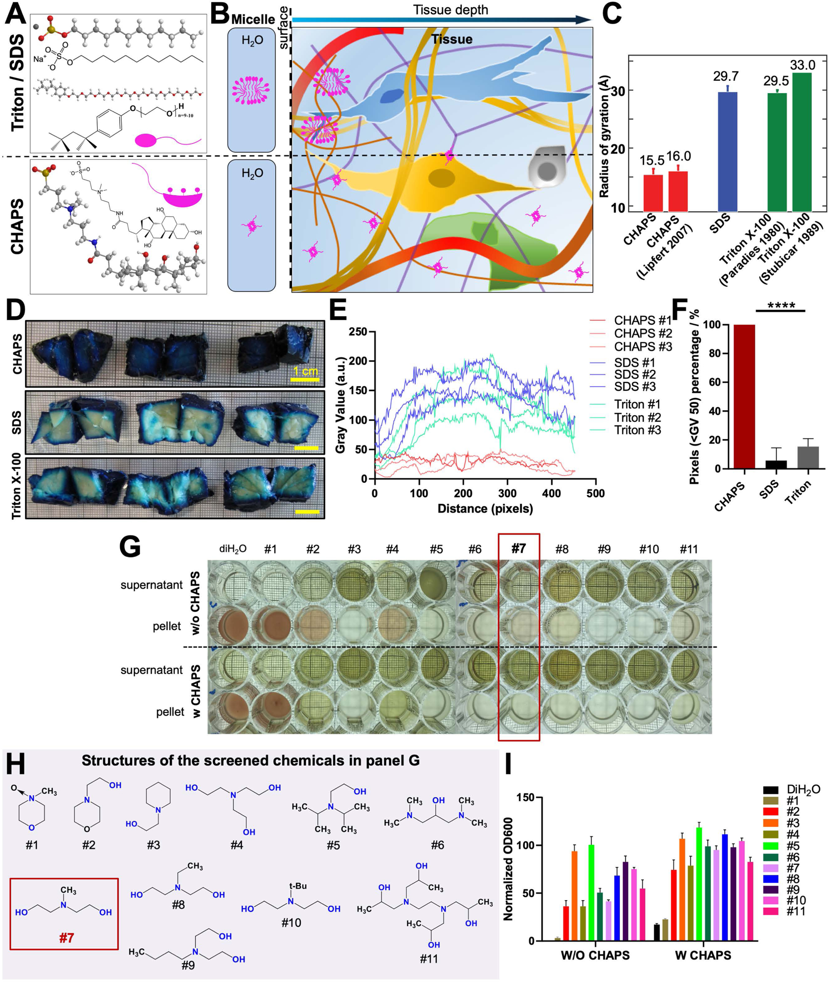
(A) 3D molecular and structural features of SDS and Triton X-100 exhibiting typical head-to-tail amphiphilicity, whereas, CHAPS exhibiting peculiar facial amphiphilicity.

(B) Schematic diagram showing facial CHAPS could more efficiently and deeply permeabilize tissue compared to standard detergents (SDS and Triton X-100) owing to the formation of smaller micelle.

(C) Radii of gyration determined for CHAPS and SDS with their literature values (full references are in Table S1) for R_g (the size of micelle is characterized by the squared radius of gyration of the micellar core, R_g²). Values for CHAPS and SDS represent mean and standard error from at least three independent repeats.

(D) Methylene blue dye staining of pig pancreas samples (1–1.5 cm cubes) after detergents permeabilization, showing CHAPS greatly enhanced deep tissue permeabilization for dye travelling comparing with SDS or Triton X-100.

(E) Profile plot along each sample dimension in D.

(F) Quantification of the pixel numbers in E under selected threshold (Gray Value (GV) < 50) (n=3).

(G) Screening of 11 chemicals in (H) without or with CHAPS admixtures for blood decolorization (see Table S2 for the name and CAS number of the chemicals). Good candidates show green supernatant and colorless pellet. CHAPS improves the decolorization efficiency with most tested chemicals.

(I) Normalized OD600 of the supernatant corresponded well with the photocamera pictures in G (n=3).

Human organs carry residual blood clots due to several hours to days of delay until organ harvest after death. Heme in the blood causes strong autofluorescence at visible wavelengths (400–700 nm) and reduces the intensity of travelling light within the tissue, thereby impeding the full transparency of cleared organs (Tainaka et al., 2014). PFA-fixed blood was washed by detergent solutions, resulting in colorless supernatant and red pellet, indicating detergent alone was unable to remove the heme (Figure S1D). To overcome this issue, we firstly screened CHAPS compatible chemicals to elute the heme. In particular, we focused on effective, colorless and cheap chemicals to facilitate scalability to large human organs (Figure 1G–I, Figure S1E,F). Our screen showed that N-methyldiethanolamine (NMDEA) was an efficient candidate when combined with CHAPS, resulting in a completely colorless pellet from PFA-fixed blood (chemical 7 in Tables S2, and Figure S1G,H). In addition, NMDEA was the cheapest among the screened chemicals, reducing the cost when used in large amounts for intact human organs (Table S2). Compared to Triton X-100 and SDS that were used in prior clearing methods as detergents, CHAPS was faster and more successful in decolorizing mouse kidney, liver, heart, spleen and brain, suggesting a better performance for large human organs (Figure S1I). Moreover, protein loss assay indicated the superior retention of endogenous biomolecules with CHAPS, assuring a more reliable molecular investigation of intact organs (Figure S1J). Thus, we anticipated that CHAPS, by forming small micelles, could completely diffuse through intact large mammalian organs and ameliorate tissue meshes, leaving behind a fully permeabilized biological tissue for cellular and molecular phenotyping.

Development of SHANEL tissue clearing

Next, we tested the accessibility of CHAPS permeabilized large mammalian organs using tissue clearing reagents. We chose to work with organic solvent-based clearing methods because they are fast and robust in addition to inducing tissue shrinkage (Pan et al., 2016), which helps to image larger organs with the limited sample holding capacity of light-sheet microscopy. First, we cleared the intact brain of a 2-year-old adult pig by passive immersion using standard organic solvent clearing reagents (Dodt et al., 2007; Erturk et al., 2012). We found that a combination of ethanol for dehydration, dichloromethane (DCM) for delipidation, and benzyl alcohol + benzyl benzoate (BABB) for refractive index (RI) matching was highly effective in rendering the centimeters-thick pig brain transparent after CHAPS/NMDEA permeabilization and decolorization (all together represents the SHANEL clearing) (Figure 2A–C). SHANEL clearing provided rapid transparency of the ~12.0 × 7.3 × 5.0 cm size pig brain including heavily myelinated white matter, thalamus and brainstem within 1.5 months (Figure 2C). The dimensions of the pig brain after clearing became 7.5 × 5.0 × 3.3 cm, with a shrinkage ratio of ~30% in volume. With the pretreatments of CHAPS/NMDEA, SHANEL clearing showed prominent capacity to render centimeters-sized mammal organs transparent compared with other clearing methods (Figure S2A,B).

Figure 2. SHANEL clearing of brain and pancreas from an adult pig.

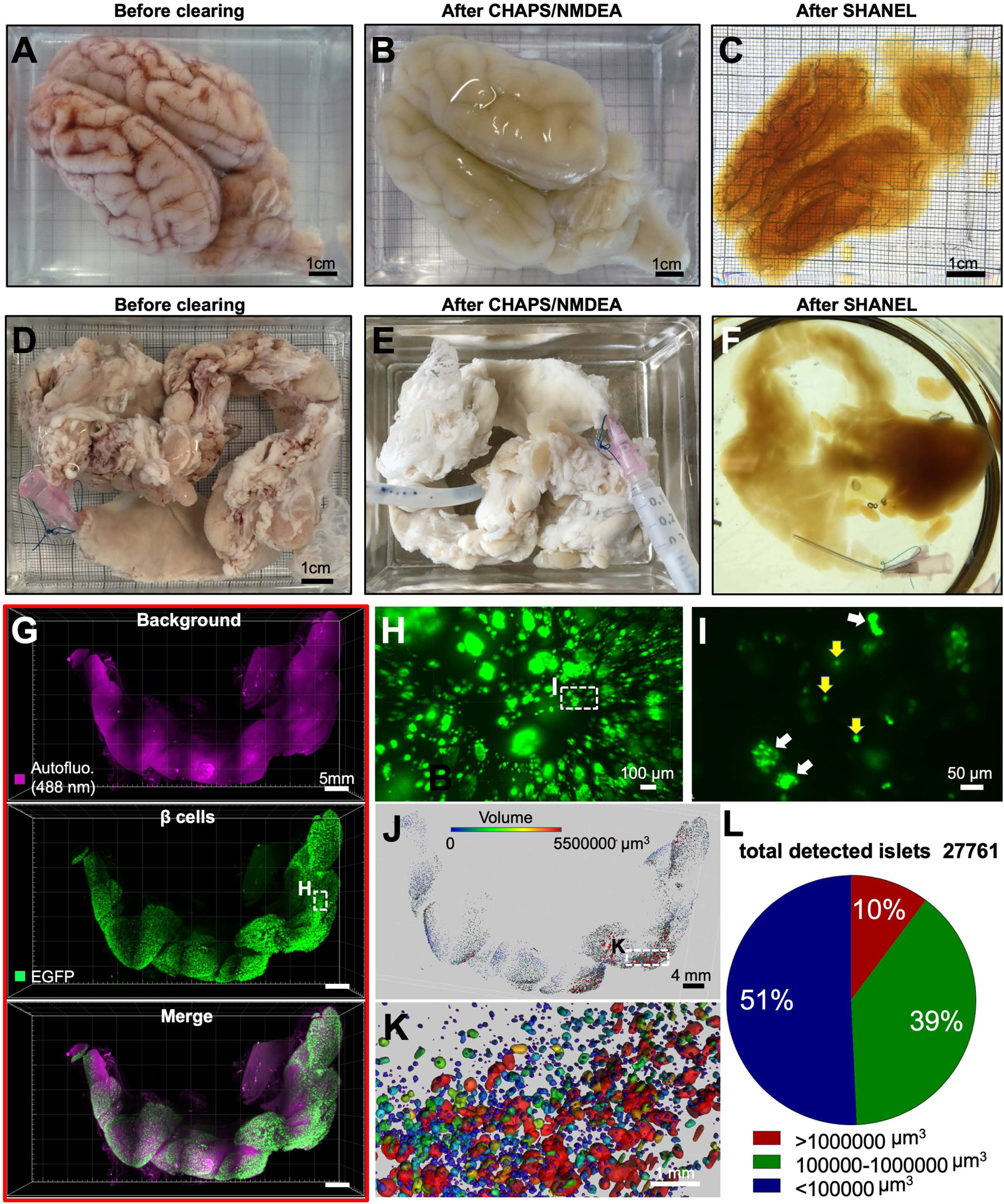
(A) PFA-fixed adult pig brain with retained blood.

(B) Permeabilized and decolorized pig brain by CHAPS/NMDEA.

(C) Fully transparent adult pig brain after SHANEL clearing.

(D) PFA-fixed, dissected (INS-EGFP transgenic pig) pancreas with retained blood.

(E) After CHAPS/NMDEA treatment, the pancreas is completely decolorized.

(F) Transparent pig pancreas after SHANEL clearing.

(G) 3D distribution of β-cell islets imaged by light-sheet microscopy after anti-EGFP nanobody boosting.

(H) High magnification view of the region marked in G (middle panel).

(I) High magnification view of the region marked in H showing β-cell islets of single cells (yellow arrows) or multiple cells (white arrows). The majority of larger islet shapes appear circular or oval.

See also Movie S1.

(J, K) Segmented 3D distribution of β-cells based on their volume in the islets of Langerhans. The heterogeneity of islet sizes is evident.

(L) Quantification of the total number of detected islets and categorization according to their volume.

Recent developments in gene editing with CRISPR/Cas9 technology have enabled the generation of large transgenic reporter mammals, expressing fluorescent proteins in the tissues of interest (Hsu et al., 2014; Kurome et al., 2017). Therefore, we applied SHANEL clearing to INS-EGFP transgenic pig pancreas exhibiting porcine insulin gene (INS) promotor driven beta-cell specific enhanced green fluorescent protein (EGFP) expression in the islets of Langerhans (Kemter et al., 2017) (Figure 2D–F). To enhance and stabilize the EGFP signal in centimeters-sized tissue, we used anti-GFP nanobodies conjugated with bright Atto dyes (Cai et al., 2018) (Figure S2C). We demonstrated that the 3D distribution of pancreatic beta cells as single cell or groups of cells within the islets of Langerhans could be readily assessed by our new approach enabling quantification of islet volume and demonstration of islet size heterogeneity (Figure 2G–L; Movie S1).

Generation of intact transparent human brain by SHANEL clearing

Labeling and clearing of the intact human brain would be a major step forward towards mapping its cellular content in the near future. As the human brain vascular system is an established network reaching all parts of the brain, we used it to deliver the chemical cocktails deep into the brain tissue (Figure S3A). We used the two main pairs of large arteries, the right and left internal carotids (CR, CL) and the right and left vertebral arteries (VR, VL) to circulate solutions. First, we used PBS/heparin solution to wash out the liquid blood, followed by 4% PFA/PBS solution to fix the brain. Subsequently, we carefully isolated the whole human brain with these major vessels and connected eyes (with a volume of ~1344 cm³ and dimensions of ~15.0 ×10.4 × 14.4 cm) from the skull. Then, we set up a pressure-driven pumping system to circulate all clearing reagents and cell nucleus labeling dye (TO-PRO-3) through the four arteries to accelerate the process (Figure 3A). By doing so, we rendered the whole adult human brain transparent for the first time. To demonstrate the full transparency, we performed the following experiments. First, we used SWIR (short-wave infrared) imaging light at 1450 nm wavelength and visualized the text through the intact cleared human brain (Figure 3B and Figure S3B) (Bruns et al., 2017; Carr et al., 2018). Second, we used a condensed white light from epifluorescence microscopy to illuminate the whole brain and observed that the light travelled end-to-end (Figure 3C). Third, we used MRI to visualize and quantify the proton density of uncleared and cleared human brain tissue, comparing the results to well-cleared mouse brain (Baek et al., 2019). The results showed that SHANEL clearing generated homogeneous tissue water replacements in both whole human brain and human brain slice, with the brain slice showing similar proton density values as the whole brain (Figure S3C). Also, the difference in proton density between cleared and uncleared human samples was similar to the mouse samples (Figure S3C). The intact transparent human brain represents a 2–3 orders of magnitude increase in the volume of sample that could be rendered transparent compared to prior methods (Hildebrand et al., 2018). The whole process including labeling and clearing takes ~4 months and costs approximately 3200 € for one adult human brain (Table S2). The final volume of the shrunken brain was 56% of the initial volume. Next, we used light-sheet microscopy to acquire mosaic images of the intact cleared human eye with a diameter of ~3 cm. We imaged TO-PRO-3 and autofluorescence signals of the intact cleared eye and reconstructed the details of its anatomical structures including sclera, iris and suspensory ligament in 3D (Figure 3D,E; Movie S2). Thus, our approach provides the basis for 3D histological assessment of the whole human brain in the near future.

Figure 3. SHANEL clearing of intact adult human brain.

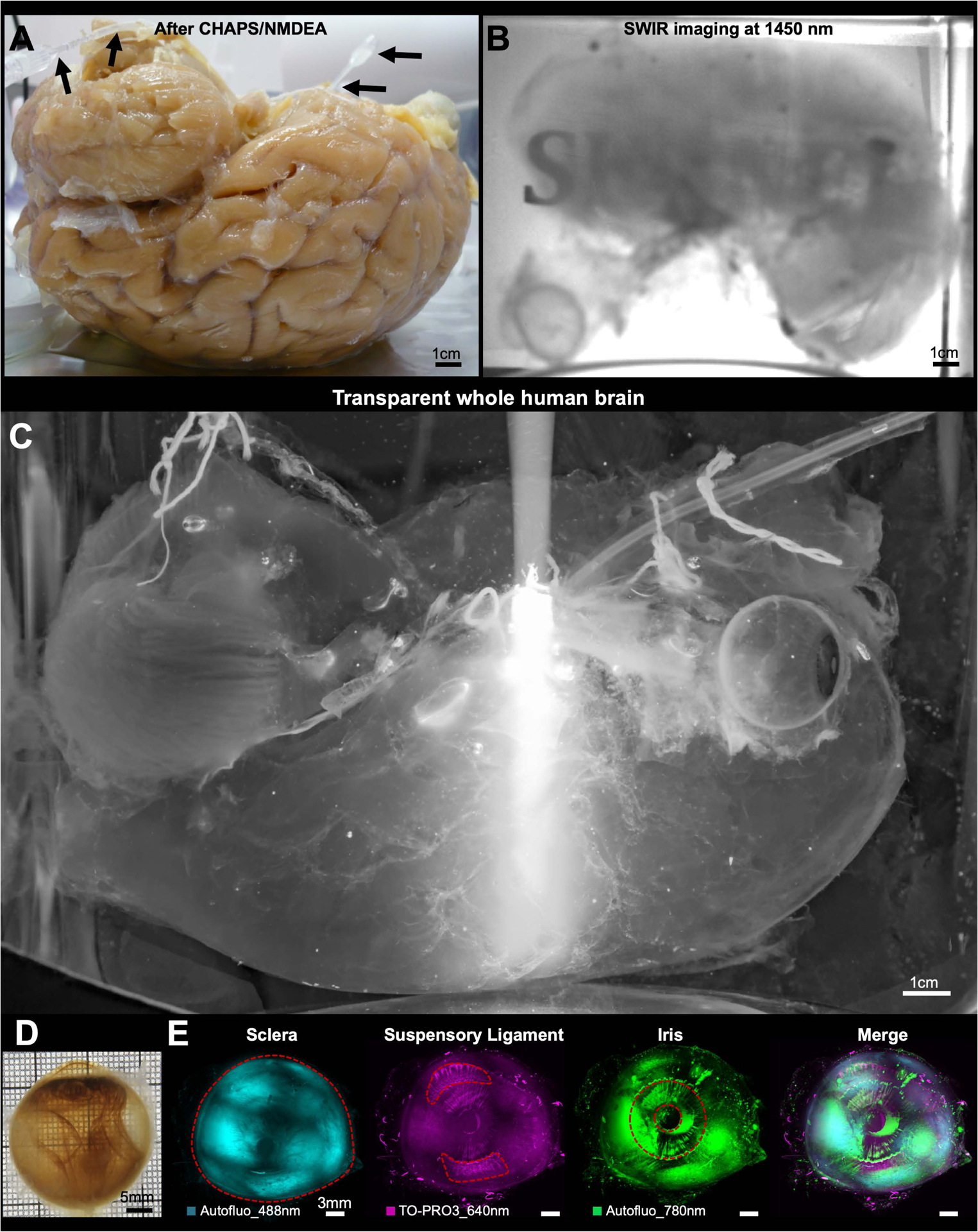
(A) A sample of permeabilized and decolorized intact adult human brain by CHAPS/NMDEA via active pumping setup (black arrows).

(B) SHANEL letters are visible, through the transparent whole human brain illuminated with 1450 nm short-wave infrared (SWIR) light.

(C) Light of epifluorescent microscope can travel in the brain end-to-end, demonstrating the full transparency of intact human brain, which has volume of ~1344 cm³ and dimensions of ~15.0 × 10.4 × 14.4 cm.

(D) Camera picture of an eye, dissected from the intact transparent human brain.

(E) 3D reconstruction from light-sheet microscopy scans of the eye showing the sclera, suspensory ligament and iris structures.

See also Movie S2.

SHANEL histology of centimeters-sized human organs

Because in vivo genetic labeling and fluorescent dye tracing are not applicable to study post-mortem human tissue, cellular and molecular interrogation of human organs requires post-mortem staining using dyes and antibodies. However, state-of-the-art antibody labeling techniques of decades-aged human samples are limited to ≤50 μm thickness in standard histology, and to a maximum of ~1 mm thickness in prior clearing methods, mainly due to the weak permeabilization of the tissue and slow diffusion of the standard antibodies (~150 kDa) (Lai et al., 2018; Murray et al., 2015; Park et al., 2018). In addition, age-related accumulation of highly autofluorescent molecules increases the background substantially in thicker tissues (Davis et al., 2014). To overcome these limitations and achieve staining of centimeters-sized human brain, we set out to develop a deep-tissue antibody labeling method. Towards this goal, we perfused an intact human brain from a 92 years old female body donor using CHAPS/NMDEA to permeabilize and decolorize. This treatment softened the sturdy human brain and allowed its easy sectioning into 12 coronal slices (each 1.5 cm thick) using a brain slicer (Figure S3D–F). The permeabilized human brain slice was further slackened by delipidation using DCM/MeOH (methanol). Next, we identified acetic acid and guanidine hydrochloride as powerful reagents to loosen the extracellular matrix (ECM) for the diffusion of large molecules such as antibodies (all together represents the SHANEL histology, Figure 4A–B).

Figure 4. SHANEL histology on centimeters-thick human tissues imaged by light-sheet microscopy.

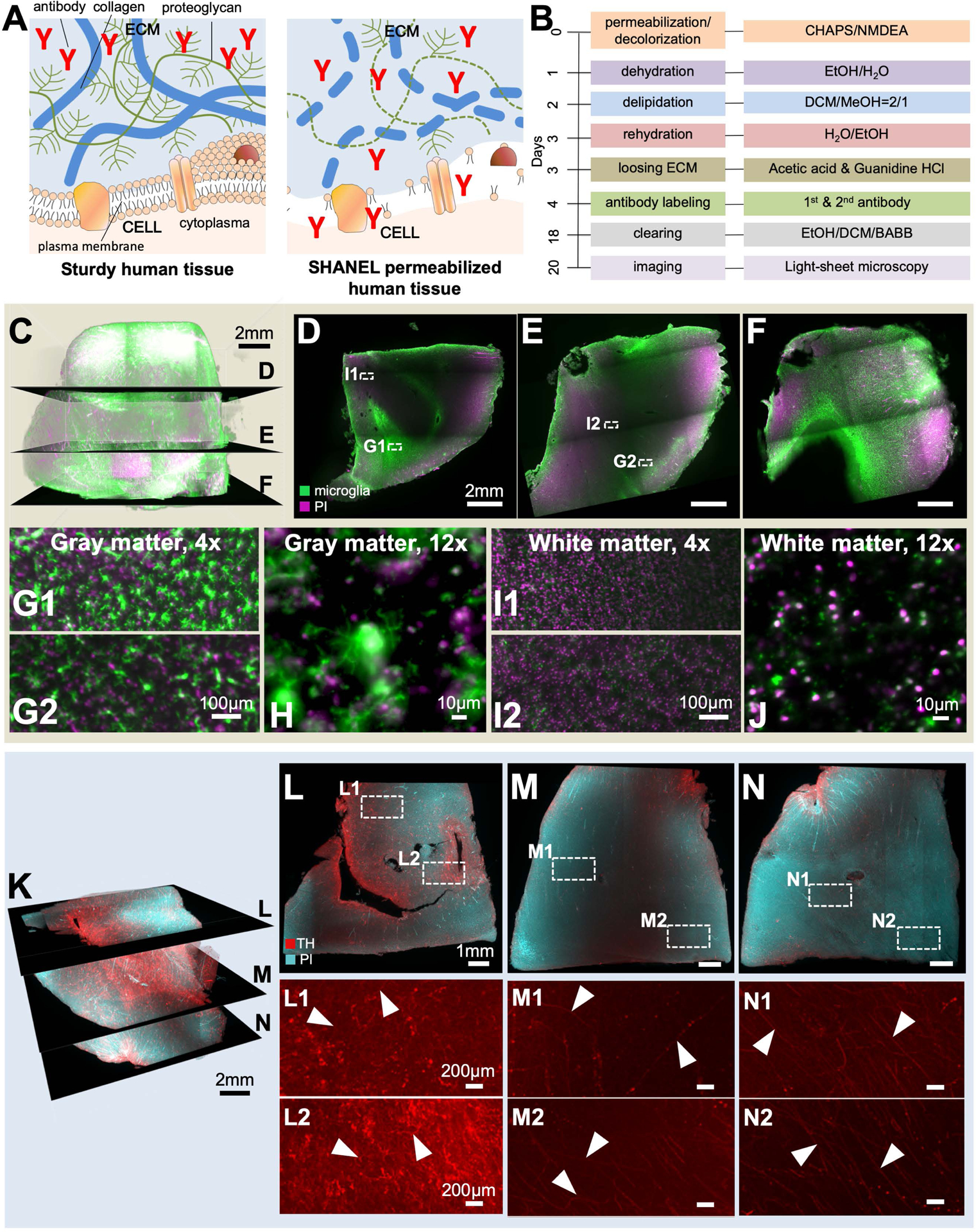
(A) SHANEL histology is further characterized by loosening extracellular matrix (ECM) and extracting lipids, which enable antibody-size molecules to fully penetrate into centimeter-thick sturdy human tissues.

(B) The step by step SHANEL histology pipeline (with durations) for deep tissue antibody labeling.

(C-F) Iba1 microglia (green) and propidium iodide (PI) (magenta) labeling of post-mortem human brain tissue with an original size of 2.0 × 1.8 × 1.5 cm (1.3 × 1.2 × 1.0 cm after shrinkage).

The differences in microglia density and morphology are evident throughout the gray matter (G, H) and white matter (I, J).

(K) Tyrosine hydroxylase (TH) (red) and propidium iodide (PI) (cyan) labeling of post-mortem human brain tissue with an original size of 1.8 × 1.8 × 1.5 cm (1.2 × 1.2 × 0.91 cm after shrinkage).

(L-N) TH+ axonal extensions in gray matter (white arrowheads in L1-L2) and white matter (white arrowheads in M1-N2) throughout the entire depth of tissue are evident. Note that cyan channel is not shown in L1-N2 to emphasize the TH labeling.

See also Movies S3.

We firstly used Methoxy-X04 (Jung et al., 2015; Klunk et al., 2002) and TO-PRO-3, which were affordable dyes in large quantities, to label Abeta plaques and cell nuclei, respectively, in an intact 16.5 × 16.5 × 1.5 cm human brain slice. After clearing, we scanned a 7.5 × 5 × 0.4 cm brain slice in ~2 days using an upright confocal microscope that is designed to scan large slices of tissue. We detected Abeta plaque accumulation in several brain regions including cingulate gyrus (CG), precuneus (PCun), superior temporal gyrus (STG) and middle temporal gyrus (MTG) (Figure S4A–D; Movie S2). We also used epifluorescence microscopy to quickly screen the 1.5 cm thick half human brain slice and again readily located the regions with Methoxy-X04-labeled Abeta accumulation for subsequent high-resolution laser-scanning microscopy (Figure S4E–H).

Antibody labeling of tissues has been widely used to interrogate the specific cellular architecture and underlying molecular mechanisms of biological processes. Therefore, we next applied SHANEL to assess the possibility of antibody-based histology of centimeters-sized human tissues. Towards this goal, we first used ionized calcium binding adaptor molecule 1 (Iba1) antibody to immunolabel microglia (Figure 4C–J) and propidium iodide (PI) to label cell nucleus. Iba1+ microglia were identifiable throughout the 2.0 × 1.8 × 1.5 cm size human brain slice (Movie S3). We also observed morphological differences: microglia cells in gray matter were mostly larger and more ramified compared to white matter (Figure 4G–J). Next, we used tyrosine hydroxylase (TH) antibody to immunolabel neuronal structures along with PI labeling of the cell nucleus (Figure 4K–N). We were able to observe specifically labeled axonal extensions throughout the 1.8 × 1.8 × 1.5 cm human brain slice (Figure 4K–N; Movie S3). These results demonstrate that SHANEL histology can successfully permeabilize the entire 1.5 cm thick sturdy human brain slices for deep tissue antibody labeling using diverse antibodies (Figure S5A). This represents a 1–2 orders of magnitude enhancement in the thickness of adult human tissue that could be processed for histology compared with prior methods (Hildebrand et al., 2018). We also found that the signal was stable for several months after SHANEL histology (Figure S5B). Studying vasculature has been a valuable method to explore diverse developmental and pathological phenomena in biological tissues. Again, histological assessment of the vasculature in human tissue has been limited by the penetration of specific vascular dyes and antibodies. Here, we used Lectin dye to effectively label a human brain sample with a size of 3.0 × 1.9 × 1.5 cm (Figure S5C). In addition to specific vascular structures (e.g. Figure S5D–F), we could identify vasculature related tissue abnormalities as swollen structures of vascular morphology (e.g. Figure S5F), which could be aneurysms, a prevalent vascular disorder affecting 25% of the population (Duan et al., 2018). 50% of intracranial aneurysms are < 5mm in diameter (Morita et al., 2012), which is in line with our observations. Thus, SHANEL histology allows the labeling of specific molecules, cells and vasculature in centimeters-sized human brain samples presenting a viable tool to scale up the investigation of brain pathologies.

Next, we tested our SHANEL technology on entire human kidneys using small molecular dyes. There is a huge shortage of organ donors for hundreds of thousands of people, whose a large portion (~55%) is waiting for kidney transplantation (Chung et al., 2014). Overall the waiting time for donation might be several years, and the cost of transplantation can reach half a million dollars (Chung et al., 2014). Understanding the 3D structure of the human kidney would be very valuable for tissue engineering efforts aiming to generate artificial kidneys using 3D-bioprinting technologies (Murphy and Atala, 2014), which require detailed cellular and molecular knowledge on intact human kidney to be replicated. Kidneys are the major organs for blood filtration through glomeruli, whose density, size and cellular integrity are critical for healthy organ function (Puelles and Bertram, 2015). Towards understanding the 3D cellular structures of the human kidney, we used SHANEL histology with active perfusion of TRITC-dextran and TO-PRO-3 dyes through the renal artery to label the vessels and dense cellular structure of the glomeruli in the entire kidney with a size of 11.5 × 8.2 × 3.0 cm. After labeling, we also actively pumped the clearing reagents through the kidney to overcome the age and size related challenges. We achieved full transparency, revealing the primary renal artery, secondary branches of segmental arteries and interlobar arteries (Figure 5A–C). Using standard light-sheet microscopy, we could visualize the 3D distribution of vessels and glomeruli in the kidney cortex over large volumes (1.2 × 1.2 × 0.45 cm), and trace individual afferent arterioles and their corresponding glomeruli (Figure 5D–F; Movie S4). Through cortex profile counting, we found that the width of the cortex zone was around 2742 ± 665 μm (mean ± s.d.), the diameter of glomerular caliper was 221± 37 μm, and afferent arteriole diameter was 71 ± 28 μm (Figure 5G).

Figure 5. Cellular investigation of human kidney.

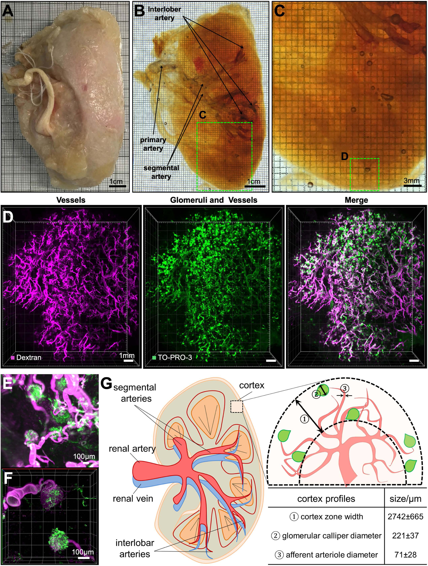
(A-C) A PFA-fixed adult human kidney (A) was rendered totally transparent after SHANEL clearing, revealing visible arteries (B,C).

(D) 3D reconstruction of vessels and glomeruli of the kidney cortex region marked in

(C) by light-sheet microscopy.

TRITC-dextran labels mostly the vessels (magenta), while TO-PRO-3 labels glomeruli more prominently (green). High magnification light-sheet microscopy (E) and confocal microscopy (F) images show the structural details of afferent arteriole (magenta) and glomeruli (green).

(G) Human kidney anatomy and cortex profiles from the 3D reconstruction. See also Movie S4.

Next, we examined whether SHANEL histology leads to tissue alterations by assessing macro- and micro-structures. The ratio-metric enlargement of shrunken tissues after SHANEL histology overlaid well with their pre-cleared images suggesting an isotropic tissue shrinkage (Figure S6A). Assessing the cellular details before and after SHANEL histology, we also did not observe a notable deformation (Figure S6B). Moreover, we also rehydrated the SHANEL-treated tissues, and performed histological assessments using H&E (Hematoxylin and Eosin), Nissl and PAS (periodic acid Schiff) stainings (Puelles et al., 2019), further confirming the integrity of cellular structures upon SHANEL (Figure S6C).

3D reconstruction of intact human organs and analysis of big data using deep learning

To enable the imaging of intact human organs, we used a prototype light-sheet microscope with extended stage movements and a large sample accommodation chamber (size of 25 × 9 × 7 cm) (Figure 6A–E). Using this new system, we scanned and reconstructed an intact human thyroid (7 × 5 × 3 cm) in 3D revealing the vessels and lymph nodes (Figure S7A–D). Also, we scanned an intact human kidney (size of 11 × 6.5 × 5 cm) end-to-end coming from a 93 years old donor (Figure 6F–I). We confirmed the transparency and imaging quality by observing the perfusion/labeling-free autofluorescence signal at 780 nm channel, which was clearly visible throughout the entire scan (Movie S4). Interestingly, we observed that a large segment of the kidney cortex had significantly reduced vascular structures appearing in 780 nm channel (Figure 6J,K, and Movies S4), which was also evident in dextran channel (Figure 6H). We also dissected exemplarily pieces and performed PAS staining to analyze the structural details. These experiments showed that the glomeruli structures were similar for both sides (Figure 6L). Overall, our data suggests a vascular pathology affecting a large segment of the kidney, which is typical of hypertensive related changes in older individuals that could potentially be preceding glomeruli pathology (Denic et al., 2017; Hughson et al., 2016). Thus, SHANEL technology can be a new tool to study pathologies of intact human organs at a gross scale proving valuable information to understand organ functions in health and disease.

Figure 6. Whole kidney imaging using Ultramicroscope Blaze with extended sample holding capacity.

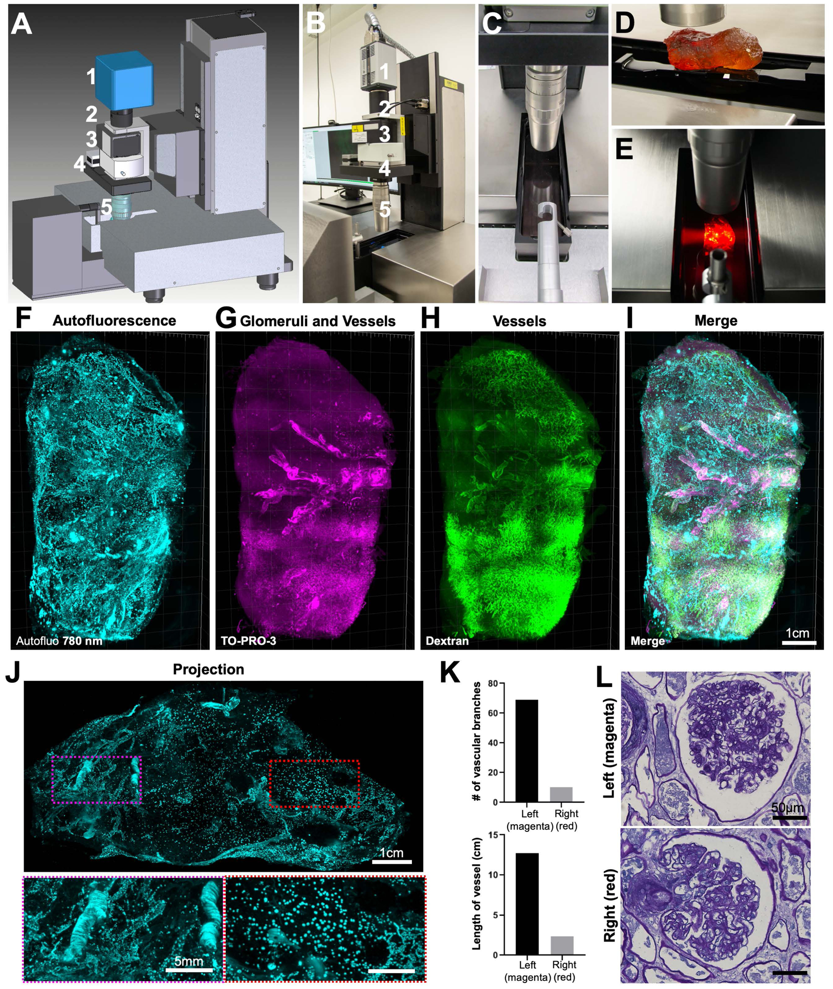
Plan (A) and picture (B) of the prototype LaVision (Miltenyi) Biotec light-sheet Ultramicroscope Blaze for large samples, featuring (1) Andor sCMOS camera, (2) tube, (3) LaVision autofocusing unit for automatic focus correction at different wavelengths, (4) zoom body, (5) 1.1x MI PLAN objective.

(C) Imaging chamber.

(D) A whole adult human kidney was mounted on the holder (note that the sample does not look transparent if not immersed in RI matching solution (BABB) as shown in the image).

(E) View of cleared whole human kidney placed in the imaging chamber with the light-sheet from the left crossing through the sample.

(F-I) 3D reconstruction of whole adult human kidney (original size of 11 × 6.5 × 5 cm) imaged by the prototype light-sheet microscope. Shown are the auto-fluorescence signal at 780 nm (F, cyan), the glomeruli and vessels from TO-PRO-3 labeling (G, magenta), the vessels from the dextran labeling (H, green), and themerged view of (F)–(H) in (I).

(J) An orthogonal 1 mm projection of the kidney showing that vascular structures are significantly reduced at the right side (red-dashed region) compared to left side of the kidney (magenta-dashed region).

See also Movie S4.

(K) Quantification of vascular features between the left (magenta) and right (red) regions of the kidney.

(L) Periodic Acid Schiff (PAS) images of rehydrated samples dissected from the left (magenta) and right (red) regions showing similar glomeruli structures for both sides.

Analyzing the large data coming from cleared tissues has remained a major obstacle (Table S3). The state-of-the-art methods for object and cell detection, for example the “3D Object Counter” tool (Bolte and Cordelieres, 2006) in the Fiji software package (Schindelin et al., 2012) and Imaris software rely on filter-based approaches such as brightness thresholding or watershed algorithms that cannot readily be scaled to analyzing terabytes of data. Recent deep learning approaches have proven to be superior for the analysis of large imaging data compared to prior methods both in terms of segmentation accuracy and computational power requirements (Belthangady and Royer, 2019; Kermany et al., 2018; Moen et al., 2019; Wainberg et al., 2018). To analyze large scale data from the cleared human tissue in a scalable and unbiased manner, we adopted a deep learning approach based on convolutional neural networks (CNNs) (Tetteh et al., 2018; Todorov et al., 2019) (Figure 7A). To generalize the efforts, we chose to focus on reliable detection, segmentation and counting millions of cells in cleared human brain tissues. Our deep learning approach consists of a CNN-based segmentation of the cells, and a connected component analysis for detecting and counting of the cells. Our CNN was ~10x faster compared to the Imaris Surface Detection Tool while they had similar accuracies on the test data patches (Figure 7B,C). Also, the CNN was 20x faster compared to the Fiji 3D Object Counter, which had a substantially lower performance (Figure 7B,C). We also tested an implementation of 3D U-Net (Çiçek et al., 2016), a common state-of-the-art CNN architecture for medical image segmentation, which performed very similar to our CNN in terms of cell detection accuracy, albeit slightly slower in processing speed (Figure 7C). Next, we applied our algorithms to 4 different large brain regions (size of ~60–145 mm³). We could readily detect, segment and map the 10–22 million cells in each brain region within a few hours (Figure 7D–G), a task that is impossible to complete with the same speed and accuracy without a deep learning approach. We designed our pipeline to be able to work on any size of scan using a standard lab workstation (e.g., with Titan T1080i GPUs). Our code is freely available at Google Colab, where the model can be tested and applied to scientists’ proprietary data in their browsers without installing any software.

Figure 7. Deep learning-based quantification of cleared human brain tissues.

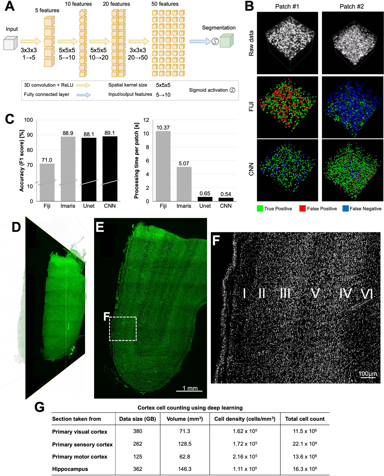
(A) The architecture of our convolutional neural network (CNN).

(B) Visual comparisons of deep learning segmentation performance to alternative automated methods on two test patches, color-coded.

(C) Comparisons of deep learning (black columns) and alternative automated methods (gray columns) for cell counting accuracy (left) and processing time (right). The cell counting accuracy is quantified as the F1 score, which represents the harmonic mean of recall (cell detection rate) and precision (false positive rate). Reported processing times were measured for the task of detecting and segmenting all cells of a 3D patch (291 μm³) on a normal workstation (32 Cores, 2 GPUs).

(D) 3D reconstruction of primary visual cortex area having ~11.5 million cells.

(E) Raw orthogonal image from the middle of D.

(F) CNN segmented image from the region marked in E. Six layers of primary visual cortex can readily be identified in CNN segmented images (100 μm projection).

(G) The summary of cell properties from different brain regions taken from cortex and hippocampus area analyzed using our CNN.

DISCUSSION

Histological studies of human tissues suffer from a lack of scalable methods to label and image large human specimens. Here we present the SHANEL method, which is derived from a new chemistry achieving thorough permeabilization of fixed post-mortem human tissues. It allows full penetration of labeling molecules and clearing chemicals into centimeters-sized decades-aged human tissues such as post-mortem human brain and kidney specimens. Our method can also readily be applied to many organs in parallel as it does not require lengthy handwork other than setting up the perfusion system and exchanging of the solutions (Table S3). Thus, this scalable method could vastly accelerate the 3D structural and molecular mapping of cells in intact human organs including the human brain.

Early efforts of adult human organ clearing started a century ago with slow progress in transparency and labeling options (Steinke and Wolff, 2001). A particular difficulty has been the age dependent accumulation of intracellular and extracellular molecules such as lipofuscin and neuromelanin pigments. Lipofuscin is a mixture of highly oxidized cross-linked macromolecules including proteins, lipids, and sugars from different cellular metabolic processes (Moreno-Garcia et al., 2018). Age-related accumulation of lipofuscin in the human body, in particular in the brain, correlates with senescence and sturdiness of human tissues (Moreno-Garcia et al., 2018). Similarly, insolubility of the collagen also increases in the human body with ageing, leading to hardening, browning and autofluorescence of the tissues (Monnier et al., 1984). Due to age-related accumulation of such insoluble macromolecules in human tissues over several decades, histological examination relying on the penetration of large molecules such as antibodies deep into tissues has been very challenging. Recently developed tissue clearing methods have proven to be a promising way to achieve histological assessment of intact specimen. While diverse clearing methods have been quite successful in rodents with the age of a few months, they have not been as effective on decades-aged human tissues. We solved this problem by developing a new method to permeabilize the sturdy human tissues, which is the prerequisite step for any tissue labeling and clearing method.

Here, we hypothesize that the micellar structures of detergents would be critical to penetrate the dense meshes of sturdy human tissues. Towards this goal, we identified CHAPS, a zwitterionic detergent having rigid steroidal structure with hydrophobic and hydrophilic faces. The ‘facial’ amphiphilicity of CHAPS is responsible for the aggregation behavior and surface configuration of molecules at interface. Firstly, CHAPS aggregates into much smaller micelles compared to standard ‘head-to-tail’ detergents such as SDS and Triton X-100, facilitating its rapid penetration deep into dense human tissues. In aggregate formation, the hydrophobic faces (β-plane of steroid) are considered to contact with each other, while the hydrophilic ones (three hydroxyl groups) remain exposing to the aqueous environment. Secondly, in terms of interfacial interaction, the facial amphiphiles bind to the bilayer in a unique mode that allows coverage of a larger hydrophobic area instead of being embedded into the bilayer. By this way, less facial amphiphile CHAPS is needed and no residual CHAPS left behind in the tissue after the treatment. Moreover, as a mild zwitterionic detergent, CHAPS exhibits better preservation of tissue endogenous biomolecules compared to SDS and Triton X-100 for cellular and molecular interrogation. Starting from this new permeabilization chemistry, we further developed our technology by loosening ECM using acetic acid and guanidine hydrochloride (Rajan et al., 2006; Yanagishita et al., 2009).

The resulting SHANEL histology method enabled diffusion of molecules as large as conventional IgG antibodies for straightforward 3D histology of centimeters-sized human organs. Thus, our approach can also tremendously help scaling up the efforts on Human Protein Atlas (HPA) by reducing the time to label and annotate across large human tissues (Sullivan et al., 2018; Vogt et al., 2018). Yet, SHANEL alone does not fully eliminate the tissue autofluorescence, in particular those coming from the lipofuscin in the brain tissue, without additional chemical treatments (Figure S7E–H). Thus, additional background signal might be observed in some of the antibody stainings. However, this autofluorescence can be used to extract more information on senescence of cells throughout different tissue layers in addition to imaging of specific dye/antibody signals in other channels. Similar to prior clearing methods using SDS and Triton, CHAPS-based SHANEL does also not preserve the lipid-base tracers such as DiI.

The SHANEL technology is also applicable to other large mammal organs. As pig is a much better model system for the human islets research compared to rodents, study of transgenic INS-EGFP pig pancreas in combination with SHANEL clearing can also accelerate research in metabolic disorders. We demonstrate that the 3D distribution of pancreatic beta cells as single cell or groups of cells within the islet of Langerhans can be readily imaged and quantified by our new approach demonstrating the islet size heterogeneity. Regional differences of islet size and distribution (head vs. tail) in human pancreas are well known, and alterations in beta cell mass occur in diverse metabolic disorders (Chen et al., 2017). For instance in disease conditions like type 2 diabetes, regional changes of islet distribution leading to preferentially large islets in the head region occur (Wang et al., 2013). Another interesting application would be to assess the quantity and distribution of porcine islets after intraportal xenotransplantation into the liver of non-human primate models (Kemter and Wolf, 2018; Wang et al., 2013).

The development of imaging systems with extended stages and imaging capacities would tremendously accelerate studies on phenotyping of the cellular and molecular architecture of the whole human organs. To start addressing this major need, here we introduced a prototype light-sheet microscope with extended stage movement and sample holding capacity, which, in principle, could accommodate and image more than ~80% of the human organs including kidney, bladder, ovaries, testes, throat, heart, thyroid, pancreas, and tongue. Imaging the entire transparent human brain on the other hand is still beyond the capacity of current microscope systems. Leading towards this possibility, Voigt et al., recently proposed the mesoSPIM (mesoscale selective plane illumination microscopy), an open-hardware microscopy platform for imaging cleared tissues several centimeters in size (Voigt et al., 2019), which could potentially be further modified to accommodate and image the whole cleared human brain. In addition, SHANEL-induced shrinkage (e.g., 44% reduction in volume for adult human brain) and usage of light-sheet microscopes with double-sided illumination could further facilitate imaging of the large cleared human samples. To test more imaging options, we sliced the intact adult human brain into twelve 1.5 cm-thick sections using standard slicer equipment and imaged with a mosaic upright confocal fluorescent microscopy. Still, such thick slices are much easier to handle compared to micrometer or even millimeter thick sections, because there is no need to embed or collect them on glass slides. Moreover, SHANEL histology allowed a thorough labeling of these 1.5 cm-thick brain slices. This allows the usage of high numerical aperture (NA) objectives such as 4x Olympus objective (NA: 0.28 and working distance (WD): 10 mm) and 20x Zeiss Clarity objective (NA: 1, WD: 5.6 mm) on defined regions of interest to reconstruct the entire 1.2 – 2 cm thick human tissue by scanning from both sides in such laser scanning systems. While the usage of high NA and high WD objectives enables ~1–2 μm resolution, this will also lead to large data in the order of at least hundreds of terabytes. It is noteworthy to mention that imaging samples as large as human brain will also benefit from imaging at near-infrared and SWIR wavelength having much better tissue penetration capabilities compared to the visible spectra used in the current light-sheet microscopes. In addition, imaging at longer wavelengths can provide further advantages in both reducing the tissue autofluorescence at the visible spectrum and multi-color imaging for which new probes are being developed (Cosco et al., 2017; Schnermann, 2017). Indeed, a near-infrared light-sheet microscopy has recently been presented (Wang et al., 2019). Imaging whole adult human kidney, we observed a large segment of the kidney lacked vascular structures at 780 nm autofluorescence channel. Our observations of the signal around the vessels, and at the fibrous capsule (outer membrane of the kidney) suggests that this autofluorescence signal could be coming from the collagen (Genovese et al., 2014; Jain et al., 2016; Manon-Jensen et al., 2016). Currently, we do not know the origin of this observed vascular changes. Another advantage of our approach is that, after SHANEL histology, the specimens become hard, enabling easy handling of complete organs and slices. Finally, owing to the complete dehydration and incubation in organic solvents, the tissues are preserved by SHANEL histology, allowing long-term storage for the future studies by the same investigators or in other labs.

The rapid progresses in tissue clearing methods and applications have introduced datasets of previously unseen sizes in mesoscale imaging. Even more limiting has been the lack of reliable methods to analyze these large datasets with conventional computational resources in moderately equipped biology labs. Here, we developed a deep learning-based framework using a CNN for the segmentation of millions of cells in cleared human brain tissue, which could not be completed without a deep learning approach at the same accuracy and speed. Here we used our pipeline to detect and segment cells in diverse brain regions. Deep learning approaches could be expanded to classify the cells, and analyze new structures such as vessels, nerves and muscles–tasks that cannot be achieved easily with traditional software packages. Thanks to the adaptability of deep learning approaches, new algorithms can be trained with a small amount of training data to perform previously unknown segmentation tasks at high accuracy and speed (Belthangady and Royer, 2019; Moen et al., 2019; Todorov et al., 2019). Deep learning methods can also be parallelized on multiple GPUs (such as using cloud computing) to quickly scale up the processing speed for data size of hundreds of terabytes.

In conclusion, this work presents a new technology to permeabilize centimeters-sized aged human tissues for molecular and cellular phenotyping. This method allows deep tissue labeling and clearing of human specimens as large as the intact human kidney and brain. Thus, in combination with light-sheet microscopy systems having extended sample scanning capacity and deep learning-based algorithms, SHANEL histology can be a key technology to map intact human organs in the near future, which would accelerate our understanding of physiological and pathological conditions governing human life.

METHODS

LEAD CONTACT AND MATERIALS AVAILABILITY

Further information and requests for resources and reagents should be directed to and will be fulfilled by the Lead Contact, Ali Ertürk (erturk@helmholtz-muenchen.de). The clearing protocols as well as cleared samples, algorithms and data on SHANEL are freely available from the Lead contact and shared at http://discotechnologies.org/SHANEL/.

EXPERIMENTAL MODEL AND SUBJECT DETAILS

Mouse samples

CD-1 IGS (Charles River, stain code: 022) mice were used for blood collection, organs screening and protein loss assay. The animals were housed under a 12/12 hours light/dark cycle. The animal experiments were conducted according to institutional guidelines: Klinikum der Universität München / Ludwig Maximilian University of Munich and after approval of the Ethical Review Board of the Government of Upper Bavaria (Regierung von Oberbayern, Munich, Germany) and in accordance with the European directive 2010/63/EU for animal research. All data are reported according to the ARRIVE criteria. Animals were randomly selected related to age and gender. Mice were deeply anesthetized using a combination of medetomidine, midazolam and fentanyl (MMF; 5 mg, 0.5 mg and 0.05 mg per kg body mass for mice; intraperitoneal). As soon as the animals did not show any pedal reflex, the chest of the animal was opened and exposed. The blood was extracted intracardially from the left ventricle. The animals were sacrificed afterwards. Then the blood was mixed with 2 times volume of 4% paraformaldehyde (PFA, pH 7.4; Morphisto, 11762.05000) in 0.01 M PBS (pH 7.4; Morphisto, 11762.01000) and incubated for 24 h at 4°C. Animals for protein loss assay were intracardially perfused with heparinized 0.01 M PBS (10 U ml−1 of heparin, Ratiopharm; ~110 mmHg pressure using a Leica Perfusion One system) for 5–10 min at room temperature until the blood was washed out, followed by 4% PFA for 10–20 min. The brains were dissected and post-fixed in 4% PFA for 1 d at 4°C and later washed with 0.01 M PBS for 10 min 3 times at room temperature.

Pig samples

An intact pig brain was bought from a local slaughterhouse and selected randomly relate to gender, then fixed for 10 days immersing it in 4% PFA at 4°C. Housing, breeding and animal experiments of INS-EGFP transgenic pigs were done at the Institute of Molecular Animal Breeding and Biotechnology at LMU Munich according to the approval of the Ethical Review Board of the Government of Upper Bavaria (Regierung von Oberbayern, Munich, Germany) and in accordance with the European directive 2010/63/EU for animal research. All data are reported according to the ARRIVE criteria. INS-EGFP transgenic pigs have a beta-cell specific EGFP reporter gene expression driven by the porcine insulin (INS) promoter (Kemter et al., 2017). Pancreas of an exsanguinated 5.5 month-old INS-EGFP transgenic male pig of a German landrace background was dissected, its pancreatic ducts were cannulated and 20 ml of ice-cold 4% PFA was slowly injected into the ducts.

Human samples

Intact human brains were taken from different human body donors with no known neuropathological diseases. All donors gave their informed and written consent to explore their cadavers for research and educational purposes, when still alive and well. The signed consents are kept at the Anatomy Institute, University of Leipzig, Germany. Institutional approval was obtained in accordance to the Saxonian Death and Funeral Act of 1994. The signed body donor consents are available on request.

The brains of a 92 years-old female and a 48 years-old male of the body donation program of the Institute of Anatomy, University of Leipzig were fixed in situ by whole head perfusion via carotid and vertebral arteries under a pressure of below 1 bar. The head was firstly perfused with 5 L heparinized 0.01 M PBS (10 U ml⁻¹ of heparin, Ratiopharm), followed by 3 L 4% PFA in 0.01 M PBS for 2–3 h. The veins were finally closí to maintain the PFA to the brain. Then the brains were recovered by calvarian dissection and preserved at least 1–2 weeks for post-fixation submersed in the 4% PFA solution. The thyroid was dissected and post-fixed by 200 ml PFA for 3 days. The kidneys of a 93 years-old female donor were dissected from the body. The blood was flushed with 200 ml of heparinized PBS in a PBS bath for 1 hr and perfused with 400 ml of PFA immersed in PFA solution. The kidneys were preserved at least 1–2 weeks for post-fixation submersed in the 4 % PFA solution at 4°C.

METHOD DETAILS

Small-angle X-ray scattering measurements

We used small-angle X-ray scattering to determine the size, shape and aggregation number of CHAPS and SDS micelles. Experimental data were collected at beam line 12ID at the Advanced Photon Source (APS) using procedures as previously described (Lipfert et al., 2007b; Oliver et al., 2013; Oliver et al., 2014). In brief, measurements were carried out with a custom-made sample cell and holder (Lipfert et al., 2006), at a temperature of 25 °C and an X-ray energy of 12 keV, with a sample-to-detector distance of 1.8 m. We defined the magnitude of momentum transfer as q = 4π / λ · sin (θ), where 2θ is the total scattering angle and λ = 1 Å the X-ray wavelength. The useable θ-range in our measurements was 0.02 Å⁻¹ < q < 0.275 Å⁻¹. Scattering angles were calibrated using a silver behenate standard sample. Data read out, normalization, and circular averaging were performed using custom routines at beam line 12ID, APS. SDS and CHAPS were measured in PBS buffer for 10 exposures of 0.1 s. Matching buffer profiles were subtracted for background correction. Subsequent exposures were compared to verify the absence of radiation damage. Horse heart cytochrome c at 8 mg/ml was used as a molecular mass standard.

Small-angle X-ray scattering data analysis

Radii of gyration R_g and forward scattering intensities I(0) were determined from Guinier analysis (Guinier, 1939; Lipfert and Doniach, 2007; Svergun and Koch, 2003) of the low q region of scattering profiles, i.e. from a fit of the logarithm of the scattering intensity vs. q² for small q (Fig. S1A–B). The fitted radii of gyration are in excellent agreement with previously reported values, as far as available (Fig. 1C). In addition, the full scattering profiles were fitted with one- and two-component ellipsoid models (Lipfert et al., 2007b) (Fig. S1C). We found that the CHAPS data were well described by a prolate one-component ellipsoid model with long axis of ≈30 Å and short axis ≈12 Å. In contrast, the SDS data require a two-component ellipsoid model for a convincing fit, similar to other ‘head-to-tail’ detergents (Lipfert et al., 2007b), and were well described by a oblate two-component ellipsoid model with an inner core (representing the region occupied by the hydrophobic tail groups) with small axis ≈15 Å and long axis ≈25 Å (in good agreement with results from neutron scattering (Hammouda, 2013)), surrounded by a shell (representing the head groups) of thickness ≈3.5 Å.

Aggregation numbers for CHAPS and SDS micelles were determined using two independent approaches (Lipfert et al., 2007b). One approach was to use the fitted geometric models to compute the volumes of the micelle (in the case of CHAPS) or of the hydrophobic core (in the case of SDS) and to compute the aggregation number by dividing the total volume by the volume of the monomer (for CHAPS, see Table S1) or the hydrophobic core volume by the volume of the alkyl tail (determined from the Tanford formula (Clarke, 1981), 350.2 ų for SDS). We note that the approach of using the micelle volume to determine the aggregation number uses the entire scattering profile in the model fit, but is independent of the scale of the scattering intensity, since only the shape of the scattering pattern is fit. An alternative and independent approach to determining the aggregation number is to determine the forward scattering intensity I(0) from Guinier analysis and to compute the aggregation number from the equation (Lipfert et al., 2007b):

$$N=I(0)/I_{\mathit{\text{mon}}}(0)=I(0)/\left[K\cdot (C-CMC)\cdot {\left({\rho }_{\text{det}}-{\rho }_{\text{sol}}\right)}^2\cdot V_{{\mathrm{mon}}^2}\right]$$

Here K is a proportionality constant that was determined from measurements of horse heart cytochrome c as a scattering standard, C is the detergent concentration, CMC the critical micelle concentration, ρ_det the electron density of the detergent, ρ_sol = 0.34 e/ų the electron density of the solvent, and V_mon the detergent monomer volume. Values for CMC, ρ_det and V_mon are given in Table S1. The approach of using I(0) to determine the aggregation number only uses the very low q information in the scattering pattern and is independent of any model assumptions about the size or shape of the micelles. Aggregation numbers determined by the independent approaches are in good agreement.

Comparison of permeabilization capacity of different detergents on pig pancreas using methylene blue dye staining

1–2 cm pig pancreas cubic samples were incubated with the following detergents: 10% w/v CHAPS (Roth, 1479.4), 10% w/v Triton X-100 (PanReac Applichem, A4975,1000) or 200mM SDS (PanReac Applichem, A2572,0250) for 2 days at 37 °C. After PBS wash, the samples were incubated with 50 ml of 0.05% methylene blue dye (Sigma, M9140) in plastic tubes (Falcon) at 37°C overnight. After PBS wash, the samples were cut into half to evaluate the staining efficiency of the inner tissue. The camera pictures of the samples were analyzed by ImageJ for profile plot along the center of the cut samples, and we quantified the pixels under threshold gray value.

Screening of affordable and scalable chemicals for blood decolorization

PFA-fixed mouse blood was thoroughly vortexed with either only 25% w/v screened chemicals (Sigma, for the catalog codes, see Table S2) or only detergents (10% w/v CHAPS, 10% w/v Triton X-100 or 200mM SDS), or the mixture of detergents and 25% w/v chemicals, and then immediately centrifuged at 15000 rpm for 5 min at room temperature. Supernatants were transferred into multi-well plates (Corning, CLS3527) and pellets were dissolved in diH₂O and also transferred into the paired wells. Camera images were immediately captured. In accordance with our hypothesis that electron-rich nitrogen donor and polarizable hydrogen of chemicals tend to bind with the iron of heme as double-action multidentate ligands, then eluting the heme from the blood, all of the tested chemicals would partly decolorize the red heme. These effects were improved with the addition of detergents. 100 μl supernatant solution from each well was transferred to a 96-well black microplate (Corning, CLS3925) and the visible spectra were recorded using a microplate reader (Fluostar Omega, BMG Labtech). The OD600 values were measured with the Omega analysis software. Considering the practical prices and availability of reagents to process large samples such as the human brain, we optimized the concentration of CHAPS with N-Methyldiethanolamine (chemical 7, Sigma, 471828) for later experiments (Tainaka et al., 2014).

Permeabilization and decolorization of mouse organs containing remaining blood

Mouse organs were dissected and post-fixed with 4% PFA/PBS from deeply anesthetized animals intended to be euthanized. The blood-rich organs were washed with PBS for 3 h × 3 times and put into a multi-well plate and camera pictures images were taken. Then the organs were incubated with the following mixtures: 10% w/v CHAPS and 25% w/v N-Methyldiethanolamine, 10% w/v Triton X-100 and 25% w/v N-Methyldiethanolamine, 200 mM SDS and 25% w/v N-Methyldiethanolamine at 37°C on a shaking rocker (IKA, 2D digital). The solutions were refreshed when the color changed to green until colorless. Then the grouped samples were washed with PBS 3 times for 3 h at room temperature and imaged again with a camera.

Protein loss assay

PFA-fixed adult mouse (3–4 months) brains were cut into 1-mm-thick sections using a vibratome (Leica, VT1200S) (Chung et al., 2013; Murray et al., 2015). All sections were weighted and randomly grouped, then placed in 5 ml solutions as follow: distilled water, 2.5% w/v CHAPS, 5% w/v CHAPS, 10% w/v CHAPS, 200 nM SDS or 10% w/v Triton X-100. The samples were incubated for 2 weeks at 37°C on a shaking rocker. The respective solutions and quantity of protein loss from the tissue which diffused into the solutions were measured using Bio-Rad DC protein assay kit (Bio-Rad, 5000116). Total protein in the mouse brain was estimated at 10% (wt). For each group, the standard solution was prepared in the same buffer as the sample.

Pig brain clearing with passive SHANEL

PFA-fixed pig brain samples were washed with PBS at room temperature in a 500 ml glass beaker and incubated with 10% w/v CHAPS and 25% w/v N-Methyldiethanolamine solution at 37°C on a shaking rocker. The incubation time for a single whole brain was 10 days, with the solution refreshed once at day 5. After the PBS washing performed at room temperature, the samples were shaken with a series of Ethanol (Merck, 10098535000)/DiH₂O solutions (50%, 70%, 100%, 100% v/v) at room temperature, followed by a DCM (Roth, KK47.1) incubation and in the end they were immersed into the BABB (benzyl benzoate:benzyl alcohol = 2:1, Sigma, W213802, 24122) solution until complete transparency. The incubation time depended on the sample size: for whole brains, 4 days for each step were needed.

Active SHANEL clearing of pig pancreas

Pancreas from a 5.5-months old INS-EGFP transgenic pig was dissected without the tail part, a G 20 venous catheter was inserted into the pancreatic duct and sewed on. 4% PFA was injected to fix the tissue, followed by post-fixation for 3 days at 4 °C. Then the sample was placed into the active pumping system consisting of a peristaltic pump (ISMATEC, REGLO Digital MS-4/8 ISM 834), chemical-resistant PTFE tubing (VWR, 228–0735) and a glass chamber (Omnilab, 5163279). After PBS washing, 200 ml solution of 5% w/v CHAPS and 12.5% w/v N-Methyldiethanolamine was circulated through the pancreas for 8 days in total, refreshing the solution with fresh one every 2 days. After 2 times of PBS washing for 3 hours, the sample was pretreated with 200 ml of permeabilization solution containing 1.5% goat serum (Gibco, 16210072), 0.5% Triton X-100, 0.5 mM of methyl-β –cyclodextrin (Sigma, 332615), 0.2% trans-1-acetyl-4-hydroxy-l-proline (Sigma, 441562) and 0.05% sodium azide (Sigma, 71290) in PBS for half day at room temperature. Subsequently, the perfusion proceeded further, through connection of a 0.20 μm syringe filter (Sartorius, 16532) to the intake-ending of the tube to prevent accumulation of dye aggregates in the sample. At the same time, an infrared lamp (Beuer, IL21) was used to heat up the solution to 26–28 °C. With this setting, the pancreas was perfused for 13 days with 250 ml of the same permeabilization solution containing 30 μl of Atto647N-conjugated anti-GFP nanobooster (Chromotek, gba647n-100, 60920001SAT2). After that, the pancreas was washed out by perfusing with a washing solution (1.5% goat serum, 0.5% Triton X-100, 0.05% of sodium azide in PBS) for 6 h 3 times at room temperature and PBS for 3 h at room temperature. The clearing was started with a series of 250 ml of Ethanol(EtOH)/DiH₂O solutions (50%, 70%, 100%, 100% v/v) pumping for 6 hours at each step. Then the pancreas was passively incubated with DCM for 1 day, proceeded by incubation into BABB solution until complete transparency in around 2 weeks.

Other clearing methods

Centimeters-sized pig pancreas, human brain and human kidney samples were cleared by 1) SHANEL without CHAPS/NMEDA pretreatment, 2) 3DISCO, 3) uDISCO, 4) vDISCO, 5) iDISCO+, 6) PACT (Passive CLARITY) and 7) MASH (RIMS=WGO/CA) protocols. 1) Samples were incubated in 50%, 70%, 100%, 100% v/v Ethanol/DiH₂O solutions at room temperature for 4h each step, followed by overnight DCM and then BABB incubation. 2) Samples were incubated in 50%, 70%, 80%, 100%, 100% v/v THF(Roth, CP82.1)/DiH2O solutions at room temperature for 4h each step, followed by overnight DCM and then dibenzyl ether (DBE, Sigma, 33630) incubation. 3) Samples were incubated in 30%, 50%, 70%, 80%, 90%, 96%, 100% v/v tert-butanol(Roth, AE16.3)/DiH₂O solutions at room temperature for 4h each step, following DCM overnight and in the end BABB. 4) Samples were incubated in permeabilization solution (1.5% goat serum, 0.5% Triton X-100, 0.5 mM methyl-β -cyclodextrin, 0.2% trans-1-acetyl-4-hydroxy-l-proline and 0.05% sodium azide in PBS) at 37°C for 1 day, then washed with washing solution (1.5% goat serum, 0.5% Triton X-100, 0.05% sodium azide in PBS) and PBS for 4 hours each. Next, the samples were treated with 50%, 70%, 80%, 100%, 100% v/v THF/DiH₂O solutions at room temperature for 4 hours each step, followed by overnight DCM and then BABB incubation. 5) We were following the latest protocol updates from https://idisco.info. Samples were incubated in 20%, 40%, 60%, 80%, 100%, 100% v/v methanol (Roth, 4627.6)/DiH₂O solutions at room temperature for 4h each step and, after chilling at 4 °C, the samples were shaken in 66%DCM/33%methanol. Then, after two washing in 100% methanol, the samples were chilled at 4°C and bleached with 5% H₂O₂ in methanol overnight. Next, samples were rehydrated with methanol/DiH₂O 80%, 60%, 40%, 20%, PBS at room temperature for 4 hours each step. Then, the samples were permeabilized with 20% DMSO and 2.3% w/v glycine solution overnight at room temperature. Last, the samples were cleared with 20%, 40%, 60%, 80%, 100%, 100% v/v methanol/DiH₂O solution for 4 hours each step, 66%DCM/33%methanol overnight, DCM 4h and DBE. 6) The samples were incubated at 4°C for 2 days in the hydrogel monomer solution of 4% acrylamide in PBS supplemented with 0.25% photoinitiator 2,2’-Azobis[2-(2-imidazolin-2-yl)propane]dihydrochloride (a.k.a VA-044, Wako Chemicals, 011–19365). Samples were degassed and incubated at 37°C for 6 hours to initiate the tissue-hydrogel hybridization. After removing the excess of hydrogel on the surface, the matrices were delipidated with 8% SDS in PBS for 5 days with shaking. Last, the samples were transferred to the RIMS media (Forty grams of Sigma D2158 (Histodenz) in 30 ml of 0.02 M PBS with 0.1% tween-20 and 0.01% sodium azide, pH to 7.5 with NaOH—which results in a final concentration of 88% Histodenz w/v). 7) MASH protocol was modified iDISCO+ protocol with another RIMS solution (WGO/CA: 72 % methyl salicylate also known as wintergreen oil (WGO, Sigma-Aldrich, 84332) and 28 % trans-Cinnamaldehyde (CA, Sigma-Aldrich, C80687).

0.5 cm thick INS-EGFP transgenic pig pancreas slices were incubated with 10% w/v CHAPS and 25% w/v N-Methyldiethanolamine solution at 37°C overnight. Half of the samples were dehydrated with EtOH/DiH₂O solutions: 50%, 70%, 100%, 100% v/v for 2 hours at each step and delipidated with DCM, then immersed into BABB solution until transparency. The other half of the samples were incubated with the permeabilization solution (1.5% goat serum, 0.5% Triton X-100, 0.5 mM methyl-β - cyclodextrin, 0.2% trans-1-acetyl-4-hydroxy-l-proline and 0.05% sodium azide in PBS) at 37°C for 5 hours, then with 10 ml of the same permeabilization solution containing 20 μl of Atto647N-conjugated anti-GFP nanobooster (Chromotek, gba647n-100) for 4 days. After that, the pancreas samples were washed with the washing solution (1.5% goat serum, 0.5% Triton X-100, 0.05% of sodium azide in PBS) for 1 hour 3 times at room temperature and then with PBS for 1 hour at room temperature. The clearing was started with a series of incubation in EtOH/DiH₂O solutions (50%, 70%, 100%, 100% v/v) for 2 hours for each step. Then, the samples were passively incubated with DCM for 1 hour, and finally treated with the BABB solution until complete transparency. The fluorescent signal was imaged with epifluorescence microscopy at designed time point.

Active SHANEL clearing of intact human brain

The four main arteries of the PFA-fixed intact human brain were connected to the ISMATEC peristaltic pump through a chemical-resistant PTFE tubing in a glass chamber. 5 L of 10% w/v CHAPS and 25% w/v N-Methyldiethanolamine solution was pumped continuously into arteries keeping the pressure at 180–230 mmHg (50–60 rpm). One channel from the pump, made by a single reference tube, was set for circulation of the solution through the artery into the brain vasculature system: one ending of the tube was connected to the tip which inserted into the artery tubing, and the other ending was immersed in the solution chamber where the brain was placed. The perfusion tip pumped appropriate solution into the artery, and the other ending collected the solution inside of the glass chamber to recirculate the solution, pumping it back into the brain. At the same time, the solution was also stirred using a blender (IKA, RCT B S000) and heated to 37–39 °C. With this setting, the human brain was perfused for one month with the solution refreshed once at day 15. Then the solution was changed to PBS for washing for 2 days. Using the same setting without heating, the human brain was labeled with TO-PRO-3 (Thermo Fisher, T3605) in 2 L PBS (1:2000 dilution) for 1 month at room temperature. After labeling the clearing was performed by perfusing with 5 L of the following series of EtOH/DiH₂O solutions: 50%, 70%, 100%, 100% v/v for one week for each step, followed by perfusion of 5 L of DCM for another week to delipidate, in the end the sample was perfused with 5 L of BABB solution until complete transparency. When the brain was getting transparent, the BABB was refreshed and the brain was stored in this solution at room temperature without further circulation or stirring.

After transparency of intact human brain, we dissected one of the eyes for 3D reconstruction using light-sheet microscopy. According to the specific signals from different channels, we identified following structures of the eye. Sclera, also known as the white of the eye, is the opaque, fibrous outer layer of the human eye containing mainly collagen and elastic fibers. Collagen and elastic fibers normally have strong autofluorescence at a wide spectra-more strongly at 488 nm and emission 540nm (Zhao et al., 2017). Iris is a thin, circular structure in the eye. Eye color is defined by the iris. The iris consists of two layers: pigmented fibrovascular layer and pigmented epithelial layer, which were visible at 640 nm and 780 nm. The 780 nm autofluorescence could come from the collagen and/or pigments as suggested (Carrim et al., 2006; Moschovakis and Highstein, 1994). Suspensory ligaments of the lens also refer to the zonule of zinn, which is mainly a collection of zonular fibers (De Maria et al., 2017; McCulloch, 1954). This eye was from a donor with blue eyes, therefore the amount of melanin present was already low. Overall, we don’t have any evidence that SHANEL removes the melanin/neuromelanin pigments.

1.5 cm-thick human brain slices preparation

PFA-fixed intact human brain was actively pumped with 5 L 10% w/v CHAPS and 25% w/v N-Methyldiethanolamine solution for one month with solution refreshed once at day 15. Then the solution was changed to PBS for active washing for 2 days. The intact human brain was cooled in PBS at 4°C overnight, then directly cut into 1.5 cm-thick slices in coronal plane using a Rotation Cutting Slicer (Rotation Schneidemaschine, Biodur, Heidelberg, Germany). The total 12 slices were serially labeled and stored in 70% EtOH at 4°C.

Passive histology of a 1.5 cm-thick intact human brain slice

A 1.5 cm-thick intact human brain slice (Number 7, see Figure S3) was randomly chosen and passively incubated with 400 ml TO-PRO-3 (1:2000 dilution) in PBS at room temperature for 1 week. Then the solution was changed to 400 ml with 100 μM of Methoxy X-04 (Tocris, 4920) in 40% EtOH (pH=10 adjusted by NaOH (Roth, 6771.1)) and the sample was incubated for another week. After labeling, the slice was washed with PBS for 1 day. The clearing started with dehydration using a series of 1 L of EtOH/DiH₂O solutions (50%, 70%, 100%, 100% v/v) and followed by delipidation using 1 L DCM. Each step lasted 1 day. Then the samples were incubated in 1 L BABB solution at room temperature until completely transparency in around 2 weeks.

Passive SHANEL antibody histology of 1.5 cm-thick human brain samples

1.5 cm-thick human brain slices (Number 4 and 6, see Figure S3) were randomly chosen and dehydrated with a series of 1 L EtOH/DiH₂O (50%, 70%, 100%, 100% v/v), then delipidated with 2 L DCM/MeOH (2:1 v/v), then rehydrated with a series of 1 L EtOH/DiH₂O (100%, 70%, 50%, 0% v/v) at room temperature. After incubating with 1 L 0.5 M acetic acid (Roth, T179.1) in DiH₂O, this solution was changed to a mixture of 4 M guanidine hydrochloride (Roth, 6069.3), 0.05 M sodium acetate (Sigma, S2889) and 2% Triton X-100 in PBS, pH=6.0, at room temperature to loosen the extra cellular matrix. The incubation time for each of all above mentioned solutions was 1 day. Next, the slices were shortly incubated with 10% w/v CHAPS and 25% w/v N-Methyldiethanolamine solution for 4 hours and washed with PBS for 1 day. The intact slices were stored in the blocking buffer (0.2% Triton X-100/10% DMSO (Roth, A994.2)/10% goat serum/PBS) at 4 °C. Regions of interest (including hippocampus, primary motor cortex, primary sensory cortex, and primary visual cortex, 2–4 cm × 2–4 cm × 1.5 cm) were cut and incubated with the same blocking buffer at 37°C for 1 day. Then the samples were incubated with rabbit antibody anti-Iba1 (1:1000, Wako, 019–19741) or rabbit antibody anti-TH (1:250, abcam, ab112) in the antibody incubation buffer (3% goat serum/3% DMSO/0.2%Tween-20/10mg∙L⁻¹Heparin/PBS) for 1 week at 37 °C. After the primary antibody incubation, samples were washed with the washing buffer (0.2%Tween-20/10mg∙L⁻¹Heparin/PBS) for 1 day refreshing 3 times and then incubated with Alexa 647-conjugated secondary antibodies (1:500, Thermo Fisher, A-21245) in the antibody incubation buffer for 1 week at 37 °C. Other samples were incubated with DyLight 649-lectin (1:500, Vector, DL-1178) in the antibody incubation buffer for 1 week at 37 °C. After washing with PBS, propidium iodide (1:100, Thermo Fisher, P3566) or TO-PRO-3 dye was added in PBS for 3 days at 37°C for cell nuclei staining. After labeling, the samples were dehydrated with a series of solutions of EtOH/DiH₂O (50%, 70%, 100%, 100% v/v) and delipidated with the DCM solution for 4 hours each solution followed by BABB incubation at room temperature until the sample transparency was reached in 2–3 days.

To test other SHANEL-compatible antibodies, we cut 1 mm thick brain slices pretreated with SHANEL histology using the vibratome, and we stained them with the following primary antibodies: mouse antibody anti-MBP (myelin basic protein) (1:250, atlas antibodies, AMAb91064), rabbit antibody anti-Laminin (1:100, Sigma, L9393), rabbit antibody anti-Neuropeptide Y (1:300, abcam, ab30914), then the incubation was performed with the respective secondary antibodies (1:500, Thermo Fisher, A-21245) for overnight. After washing with PBS, propidium iodide (1:100) was added in PBS for cell nuclei staining for 1 hour. The samples were dehydrated with a series of solutions of EtOH/DiH₂O (50%, 70%, 100%, 100% v/v) and delipidated with DCM solution for 1 hour each solution. BABB solution replaced the DCM solution and the samples were incubated in BABB at room temperature until complete transparency.

To evaluate the macroscopic and microscopic deformation after SHANEL clearing, we used 1 mm thick human brain slices. The gross shape of the samples was imaged by the Zeiss AxioZoom EMS3/SyCoP3 epifluorescence stereomicroscope before and after SHANEL clearing. For the evaluation of the deformation at the microscopic level, samples were labeled to highlight cellular structures: in particular microglia and astrocytes in the samples were stained using the primary rabbit antibody anti-Iba1 (1:1000, Wako, 019–19741), and the primary rabbit antibody anti-GFAP (1:1000, Dako, Z033401–2) respectively, followed by the secondary antibody Alexa 647 goat anti-rabbit (1:500, Life Technology, A31852) using the SHANEL histology protocol (see previous sections). Subsequently, same regions before and after clearing of the labeled slices were imaged with the Zeiss confocal microscope LSM 880 coupled with a 25x water-immersion long working distance objective (Leica, 0.95 NA, WD = 2.5 mm) mounted on a custom mounting thread. The mounting of the slices for the imaging session was done by putting the individual samples on the glass surface of 35 mm glass-bottom petri dishes (MatTek, P35G-0–14-C) for both epifluorescence and confocal microscopy. Closing or sealing of the petri dish was not needed. These confocal scans were later used for the calculation of the root mean square error (see next section).

A second experiment to demonstrate the preservation of cellular and tissue morphology after SHANEL was performed as follows: SHANEL histology cleared human brain and kidney pieces were rehydrated with DCM, EtOH/diH₂O (100%, 70%, 50%) and PBS. These rehydrated samples together with PFA-fixed samples were cut into 20 μm thin slices using a cryostat (Cryostar NX70, Thermo Fisher) for standard hematoxylin and eosin (H&E), Nissl, Periodic Acid Schiff (PAS) staining to qualitatively assess the cellular and extracellular matrix structures with and without SHANEL histology clearing. Hematoxylin-eosin staining was carried out as follows: cryosections were passed through 2 diH2O steps before incubating in Gilĺs hematoxylin solution (Sigma-Aldrich, GHS3) for 90 seconds followed by washing under running tap water. Subsequently, cryosections were passed through a battery of increasing concentration of ethanol (50%, 70%, 80% v/v, 2 min each) and then incubated in eosin solution 1% (Roth, 7089.1) for 3 min, followed by 3 quick washes in 96% ethanol and dehydration for 2 times 5 min each in absolute ethanol and Roti-Histol 100% (Roth, 6640.2). Cryosections were then mounted in hydrophobic mounting medium (Sigma-Aldrich, Eukitt 03989) and let dry until imaging. For Nissl staining, cryosections were incubated for 2 min in 70% ethanol prior to incubation in cresyl violet solution 0.5% (Sigma-Aldrich, C5042) for 15 minutes. Following that, slides were quickly washed in distillated water twice and then passed quickly through increasing concentrations of ethanol (70%, 96%, 100% v/v), followed by incubation for 2 min in 100% isopropanol and final dehydration in 100% Roti-Histol twice for 5 minutes. Slides were mounted as described previously. Periodic acid shift staining was performed using PAS staining system (Sigma-Aldrich, 395B) according to manufacturer’s instructions. In brief, hydrated cryosections were incubated for 5 minutes in periodic acid solution and then rinsed several times in diH₂O, followed by incubation in Schiffś reagent for 15 min. After washing under running tap water, slides were counterstained in Gilĺs Hematoxylin for 90 seconds and subsequently dehydrated and mounted as stated earlier. Image acquisition was performed with an AXIO Imager.M2 microscope (Zeiss) couple with AXIOCam MRc camera (Zeiss) and a EC Pan-NEOFLUAR 40x/0,75(NA) M27 WD:0.71 mm dry objective (Zeiss, 420360–9900).

Copper sulphate treatment in SHANEL to eliminate tissue autofluorescence

1 mm thick human brain slices were cut using the vibratome after SHANEL histology pretreatment. Slices were cleared and imaged with light-sheet microscopy in different wavelengths for autofluorescence. Then, the slices were rehydrated with a series of solutions: 5 ml EtOH/DiH₂O (100%, 70%, 50%, 0% v/v) into water, 1 hour each step, and incubated with 10 mM copper sulphate (CuSO₄, Roth, CP86.1) and 50 mM ammonium chloride (Roth, P726.1) pH=5.0 solution for 1 hour at room temperature. After washing with PBS, the slices were cleared again and imaged with light-sheet microscopy at the same wavelengths used before to check the grade of autofluorescence elimination after the copper sulphate treatment. The images were then analyzed by Image J for profile plots and signal intensity. We also processed slices labeled with DyLight 649-lectin and propidium iodide with the same autofluorescence-elimination procedure to check that copper sulphate treatment did not affect the fluorescence signal from the staining while eliminating the autofluorescence from the tissue.

Passive SHANEL histology of intact human thyroid

A thyroid from an 80 years-old female donor was dissected and post-fixed with PFA for 3 days. After PBS wash for 4 hours at room temperature, the thyroid was incubated at 37°C in 200 ml of a 10% w/v CHAPS and 25% w/v N-Methyldiethanolamine solution for 5 days refreshing once at day 3. Then the dehydration of the sample was done with a series of solutions: 200 ml EtOH/DiH₂O (50%, 70%, 100%, 100% v/v), half day each solution, followed by delipidation with 200 ml DCM/MeOH (2:1 v/v) for 2 days in a sealed glass container, and rehydrating with a series of solutions: 200 ml EtOH/DiH₂O (100%, 70%, 50%, 0% v/v) half day each solution. The ECM was loosened with 0.5 M acetic acid in PBS for 1 day and a mixture of 4 M guanidine hydrochloride, 0.05 M sodium acetate and 2% Triton X-100 in PBS, pH=6.0, for 1 day. After PBS wash, 100 ml of TO-PRO-3 dye (1:1000) was used to label the sample for 10 days. The clearing was started incubating the sample in a series solutions consisting of 200 ml of EtOH/DiH₂O solutions (50%, 70%, 100%, 100% v/v), shaking for half day each step, followed by 200 ml of DCM for 5 hours, then proceeded with 200 ml BABB solution until complete transparency reached in 3–5 days.

Active SHANEL histology study of intact human kidney

The PFA-fixed intact kidneys were pumped through primary artery with 36 ml of the mixture of 25 mg/ml tetramethylrhodamine isothiocyabate-dextran, 2 mM p-maleimidophenyl isocyanate (PMPI) and 5 mM DL-dithiothreitol (DTT) in PBS (Annunziato et al., 1993; Shen et al., 2004). Then the kidneys were sealed inside a plastic bag and incubated in 37°C overnight. After dextran labeling, we set up the perfusion system with an ismatec peristaltic pump and PTFE tubing at room temperature as the human brain. The first step consisted of the washing with 2 L PBS for one day twice. The second step was the decolorization and permeabilization steps performed with 2 L of the 10% w/v CHAPS and 25% w/v N-Methyldiethanolamine solution for one week. The third step was the dehydration step with a series of solutions: 2 L of EtOH/DiH₂O (50%, 70%, 100% v/v), 4 days with each solution. The fourth step was the delipidation step with 4 L DCM/MeOH (2:1 v/v) for 4 days, by sealing the glass container. The fifth step was the rehydration with a series of solutions: 2 L EtOH/DiH₂O (100%, 70%, 50%, 0% v/v), 4 days with each solution. The sixth step consisted of the loosening of the ECM with 0.5 M acetic acid for 4 days and mixture of 4 M guanidine hydrochloride, 0.05 M sodium acetate and 2% Triton X-100 in PBS pH=6.0, for 4 days. The seventh step was again PBS washing for one day twice. Next, 1 L of TO-PRO-3 dye (1:2000) in PBS was continuously pumped for 2 weeks, then washed with PBS for one day twice. The clearing was started with a series solutions consisting of 2 L of EtOH/DiH₂O solutions (50%, 70%, 100%, 100% v/v) pumping for 2 days for each solution, followed by 2 L of DCM for 3 days, then proceeded with 2 L BABB solution until complete transparency.

To examine the whole kidney pathology, we used tissue recycling reported in details in (Puelles et al., 2019). Briefly, the concept is based on reversing the main clearing steps. Thus, after SHANEL, BABB-immersed tissues were gently placed in sequential washes of 100% ethanol, 30 minutes each, 3–5 times (depending on tissue size). Next, sequential washes in PBS were performed, 30 minutes each, 5 times to get rid of residual BABB. Then, conventional paraffin embedding and slicing (5 μm thick) was carried out, thereby allowing subsequent PAS staining as previously described.

To quantify the vessel structures in normal and reduced areas, 8 mm projection (200–1200 slices) of 780nm autofluorescence signal of whole kidney was evaluated by counting the vessel branches and length in same size areas using Image J.

Safety recommendations of handling chemicals

According to the open chemistry database from National Institute of Health (NIH) through PubMed, we summarized the safety recommendations of handling SHANEL chemicals. CHAPS is not a hazard substance. It will cause skin and eye irritation and may cause respiratory irritation. NMDEA will cause eye irritation. EtOH is highly flammable liquid. DCM will cause skin, eye and nose irritation, and in case of inhalation, it could cause anesthetic effects, nausea and drunkenness. Benzyl benzoate is harmful if swallowed, and cause skin and eye irritation. Benzyl alcohol is harmful is swallowed and inhaled. However, it meets Safer Choice Criteria for its functional ingredient-class. According to the American Food and Drug Administration (FDA), both benzyl alcohol and benzyl benzoate can be used in minimum quantity as food additive or cosmetic ingredient for human use and consumption. Storing SHANEL chemicals must follow dispositions for hazardous, inflammable, explosive and toxic substances. In particular, handling must be performed in fume hoods, while wearing safety goggles, nitrile gloves (preferably double layer) and lab coats.

SWIR imaging

The cleared human brain was placed in a rectangular glass jar filled with BABB. The jar was positioned between a 1450nm LED light source (Thorlabs, M1450L3) and a cooled InGaAs camera (Allied Vision, G-032 cool TEC2) equipped with a 35mm objective lens (Navitar, SWIR-35). Homogeneous illumination of the sample was established with the help of an engineered diffuser (Thorlabs, ED1-S50) after the collimated LED and plastic diffuser foils at the illuminated side of the glass jar. Two aligned laser printed transparencies with the “SHANEL” lettering were placed between the diffuser foils and the glass wall. Images were taken at 40ms exposure time in high gain mode (gain 1).

An overhead projector (A+K lux) with a 250W halogen light bulb was used for transmissive illumination of the cleared and uncleared 1.5 cm thick human brain slices. Samples were imaged in glass dishes containing BABB and DCM for the cleared and uncleared samples, respectively. SWIR images where taken with a cooled InGaAs camera (Allied Vision, G-032 cool TEC2) together with a 35mm objective lens (Navitar, SWIR-35) equipped with a 1450/50nm bandpass (Edmund optics 85–901) mounted in front of the objective, 54μs exposure time, gain 0. Visible light images where taken with a silicon industry camera (IDS UI3370CP-NIR) together with a 35mm objective lens (Spacecom VHF 35-MP SWIR), 800μs exposure time.

Proton density MRI imaging

Quantitative MRI experiments were conducted to determine the chemical constitution of uncleared and cleared brain samples as assessed by proton density imaging. Uncleared samples in PBS or cleared samples in BABB were separately encapsulated in Eppendorf tubes (mouse brains) or sealed plastic bags (human brains), which in turn were put in a lager container with 1.5% agarose gel as reference. For all samples, we used a T2-weighted multi-echo spin echo sequence for relaxometry. For animal samples, images were acquired on a Mediso NanoScan 3T (Mediso Medical Imaging Systems, Budapest, Hungary) with repetition time 3850 ms, delta-echo-time 15 ms, 12 echos, field-of-view 16 mm × 16 mm, matrix 96 × 96 and slice thickness 1 mm. For human samples, images were acquired on a Siemens Magnetom Prisma (Siemens Healthineers, Erlangen, Germany) with repetition time 1000 ms, delta-echo-time 15 ms, 15 echos, field-of-view 256 mm × 256 mm, matrix 320 × 320 and slice thickness 1 mm. In order to determine proton density signal (S0), a logarithmic curve was fit to the signal decay measured along the multiple echoes, using MATLAB. S0 was then extrapolated as the fitted T2 signal amplitude at TE = 0 ms. The resulting S0 was normalized to S0 in the 1.5% agarose gel for comparison across the samples.

Light-sheet microscopy imaging

Single plane illuminated (light-sheet) image stacks were acquired using the light-sheet microscopes: Ultramicroscope II featuring the following filter sets: ex 470/40 nm, em 535/50 nm; ex 545/25 nm, em 605/70 nm; ex 580/25 nm, em 625/30 nm; ex 640/40 nm, em 690/50 nm; ex 780 nm, em 845/55 nm; and a prototype Ultramicroscope featuring the following filter sets: ex 470 nm, em 525/50 nm; ex 561 nm, em 595/40 nm; ex 640 nm, em 680/30 nm; ex 785 nm, em 845/55 nm (LaVision BioTec). Samples (detailed information in Table S3) were imaged with a 1x Olympus air objective (Olympus MV PLAPO 1x/0.25 NA [WD = 65mm]) coupled to an Olympus MVX10 zoom body, which provided zoom-out and -in ranging from 0.63x up to 6.3x. Alternatively, the samples were scanned with a dipping 1.1x objective (LaVision BioTec MI PLAN 1.1x/0.1 NA [WD = 17 mm]) coupled with an Olympus revolving zoom body unit (U-TVCAC) on the prototype Ultramicroscope. After low magnification imaging of whole organs, samples were imaged using high magnification objectives (Olympus XLFLUOR 4x corrected/0.28 NA [WD = 10 mm], LaVision BioTec MI PLAN 12x/0.53 NA [WD = 10 mm]) coupled to an Olympus revolving zoom body unit (U-TVCAC) kept at 1x. Tile scans with 20% or 30% overlap along the longitudinal x-axis and y-axis were obtained using a z-step of 3 μm, 5 μm or 8 μm. Exposure time was 90–120 ms, laser power was adjusted depending on the intensity of the fluorescent signal (in order to avoid saturation of the signal) and the light-sheet width was kept at 80% of maximum. The LaVision light-sheet microscope has ~4 μm lateral and ~6.5 μm axial resolutions (1x objective).

Laser-scanning confocal microscopy imaging

We used different kinds of confocal microscopes: the Zeiss LSM 880 confocal microscope was used for method characterization experiments and the imaging of regions of interest from the samples (1 mm thick, 5–10 mm long) already imaged with light-sheet microscopy. In particular, areas of interest from the human brain and the human kidney, were dissected and imaged with this inverted laser-scanning Zeiss confocal microscope using Zen 2 software (v.10.0.4.910; Carl Zeiss AG). Before imaging, samples were mounted by placing them onto the glass surface of 35 mm MatTek glass-bottom petri dishes while adding a few drops of BABB to make sure that the imaging region was immersed in BABB (Cai et al., 2018). The imaging was done using a 40x oil-immersion objective (Zeiss, ECPlan-NeoFluar × 40/1.30 oil DIC M27, 1.3 NA [WD = 0.21 mm]) and a 25x objective (Leica, 0.95 NA [WD = 2.5 mm]) mounted on a custom thread.

The second confocal microscope is the upright confocal microscope RSG4 from MAVIG. This microscope was used to image a 7.5 × 5 × 1.5 cm brain section, which was cut from the human slice number 7 previously labeled and cleared. The imaging was performed using Caliber I.D. RS-G4 research software. The working dimensions of the stage of this latter microscope were 46 × 40 × 66 cm. The images were acquired with the UPLFLN 10x objective (OLYMPUS 0.3 NA [WD = 10mm]). Tile scans were obtained along the longitudinal y-axis. Laser power was adjusted depending on the intensity of the fluorescent signal (in order to avoid saturation of the signal).

Epifluorescence stereomicroscopy imaging

Epifluorescence stereomicroscope was performed to image a cleared 1.5 cm thick whole human brain slice and 1 mm think small sections of human brain slices. The whole brain slice was put in a glass chamber while the small sections in the MatTek glass bottom dishes. The microscope was a Zeiss AxioZoom EMS3/SyCoP3 fluorescence stereomicroscopy coupled with a 1x long working distance air objective (Plan Z 1x, 0.25 NA, WD = 56 mm). The magnification was set as 32x and for the whole brain slice the imaging areas were selected manually to cover half of the slice. The images were taken with 405 nm filters and files were exported as tiff images.

QUANTIFICATION AND STATISTICAL ANALYSIS

Image processing

Processing, data analysis, 3D rendering and video generation for the imaging data were done on an HP workstation Z840, with 8 core Xeon processor, 196 GB RAM, and Nvidia Quadro k5000 graphics card and HP workstation Z840 dual Xeon 256 GB DDR4 RAM, nVidia Quadro M5000 8GB graphic card. We used Imaris (v.9.1, Bitplane), Arivis, Photoshop (Adobe, CC2018) and Fiji for 3D and 2D image visualization. 16-bit grayscale TIFF images for each channel were separately acquired by the light-sheet microscope software ImSpector (v.5.295, LaVision BioTec). Tile scans were stitched by Fiji’s stitching plugin49. Stitched images (Figure 2G–I; Figure 3D,E; Figure 4C–N; Figure 5D–E; Figure 6F–J; Figure 7D–E; Figure S4B–H; Figure S5B–F; Figure S7B–D) were saved in TIFF format and optionally compressed in LZW format to enable fast processing. To merge the neighboring stacks, alignment was done by manually selecting 3 anatomic landmarks from the overlapping regions. The stitching was performed sequentially with the Scope Fusion module of the Vision4D (v.2.12.6 × 64, Arivis) software. Landmarks were mainly chosen from the cellular structures or vessel structures on the basis of visual inspection of the anatomical features. Please note that the apparent borders (dimmer lines) typically appear at the stitching lines of the mesoscale light-sheet imaging due to overlapping scan of the same region, which can reduce the signal intensity of borders (e.g., Figure S4K–N). In addition, some blocks might appear brighter or darker in mesoscale imaging due to 1) long distance travel of light-sheets from left and right, which cannot be equal all the time at different points, 2) a blockage of one of the light-sheets (e.g., Figure 7E) and 3) lack of imaging data at certain positions (e.g., Figure S4E). However, such artefacts does not impede 3D-visualzation. After finishing the 3D reconstructions, the data visualization was done with Imaris in both volumetric and maximum-intensity projection color mapping. Epifluorescence stereomicroscopy images were saved as series TIFF images. The images were stitched manually in Photoshop by overlapping regions from landmarks.

Tissue deformation analysis using RMSE calculation

The grade of the deformation of the tissue caused by SHANEL was assessed visually on the microscopy images and by using the calculation of the Root Mean Square Error (RMSE) that evaluated the morphological deformation of the tissue structures at single-cell level. We applied the same calculation method on 2 different cell types: microglia expressing Iba1 and astrocytes expressing GFAP. To do so, first we imaged the same cells with the Zeiss LSM 880 confocal microscope (see confocal microscopy imaging section) in the samples before and after SHANEL clearing (n=3 tissue slices per each cell type), then we selected the images (maximum intensity projections) of at least 4 individual cells per each experimental replicate before and after SHANEL clearing, to compare the after-clearing cellular morphology to the corresponding one before the clearing. All the selected images were preprocessed in Fiji using background subtraction (radius 30) and median filtering (radius 2) functions in order to remove artifacts and ease the registration process. Then in the same software, images were scaled up by a factor of 2. Since the clearing process shrinks the samples, we performed a similarity registration to approximately scale the cells from after-clearing samples to match the size of the same cells before-clearing. In this way the RMSE will be calculated on scale-matched images and since the shrinkage effect will not be then considered after the scale matching, the result will be an indication of the grade of the isotropicity of the shrinkage and of the deformation that SHANEL might cause. The similarity transformation was performed using linear stack alignment with SIFT plugin.

Next, we calculated the deformation of the structures of each cell after-clearing over the structures of the same cell before-clearing. To do so, we used a non-rigid Bspline registration, from the Fiji plugin “bUnwarpJ” to align the two cell images with the following parameters: registration mode→ accurate, initial deformation → coarse and saving the transformation. To achieve better results, a couple of cellular structures were manually selected as landmarks. We could then visualize this registration as a deformation space or a deformation field, the latter indicated how much each pixel was transformed (how big the error) to match the destination image. The single spot where the deformation field showed minimal value was chosen as center of the cell for the subsequent analysis, therefore its coordinates were taken. To calculate the deformation, we converted the Bspline transformation to raw transformation using “bUnwarpJ”: in this step the RMSE was calculated for each pixel. However, in order to calculate this change in morphology (considering RMSE) only for the pixels representing the cells, in Fiji we created a binary image that separated cells from the background by using the “convert to mask” function. Afterwards the skeleton image of the cell representing the gross morphology of the cell was created in python using the skeletonize function from the skimage library. We masked the deformation image with the skeleton image giving as output the deformation image of the skeleton. In the end, we calculated the grade of deformation in term of RMSE considering sequential distances away from the previously selected cell center: the radial profile for the deformation was calculated step by step at defined increasing distances from the cell center. We binned the pixels based on their distances from the cell center and calculated the average and the standard deviation of the RMSE of the all pixels falling inside each distance range. These results were then aggregated for the total analysis taking into account all cells considered per each replicate, then the averaged result of the 3 replicates and their standard deviations were displayed together as radial profiles shown in the Supplementary Figure 6. The analysis procedure from the skeletonization step could be automatized using a scripting language such as Python or Matlab.

3D volume and iso-surface rendering and quantification of pig pancreas islets

Insulin positive β-cell volumes were quantified by 3D iso-surfacing using the Imaris software. In the software islet volumes were segmented using the ‘absolute threshold’ thresholding option and the intensity threshold was set manually for most of the pancreas with the filter of ‘number of voxels Img=1’. Statistical data parameters (Overall, Area, Center of Homogeneous Mass, Ellipsoid Axis A, Ellipsoid AxisB, Ellipsoid Axis C, Ellipsoid Axis Length A, Ellipsoid Axis Length B, Ellipsoid Axis Length C, Ellipticity (oblate), Ellipticity (prolate), Number of Voxels, Position, Sphericity and Volume) were exported from Imaris into an Office Excel (14.0.6023.1000, Microsoft, 2010)) spread sheet (*.xls). Statistical analysis of the islet volumes was performed using GraphPad Prism8.

Cell detection and image analysis

General data processing

Data processing after image stitching was performed using Python as well as various libraries such as Scipy (Virtanen et al., 2019), Numpy (Van Der Walt et al., 2011), Pandas (McKinney, 2010) and Nibabel (Brett et al., 2016). Deep learning algorithms were implemented in PyTorch (Paszke et al., 2019). To enable memory efficient and parallel patch-wise processing, the obtained 3D scans were subdivided into neighboring patches of (100 px)³ (around 4MB file size uncompressed). Patches overlapped 5% in all directions (corresponding to 15% volumetric overlap) to ensure no cell would be divided at a patch boundary. Subsequent re-concatenation rules out double counting of any cells.

Selection of data

In total four different sections of the human brain have been selected for our deep learning pipeline. One section was chosen from the human hippocampus and three sections from the cortex region, namely the areas of the cortex connected to visual, motor and sensory tasks. These scans were acquired with a 12x objective using light-sheet microscope. The x-y-resolution of this scan is 0.54 μm × 0.54 μm and the z-step is 5μm. In total, 278656 patches from the human brain scan were processed.

Data annotation

In order to have a meaningful sample of our complete dataset, representative patches from 12 locations were selected for data annotation. We chose 6 locations from the hippocampus section and 2 locations from each of the three cortex sections. In each location, 8 neighboring patches were sampled for a total of 96 patches. The ground truth annotation was performed by four human experts in this field. These annotations were used for training our deep learning models as well as evaluating and comparing the performance of each method (see below for details). Every cell in a patch has been annotated by marking the core region of the cell in ITKSnap (Yushkevich et al., 2016). Afterwards, an independent expert reviewed each patch individually to make sure that the annotation was consistent. This revision resulted in the manual refinement of 24 patches until the result was deemed correct.

Non-deep learning approaches to cell counting

Approach 1: FIJI

Fiji is an image processing package for scientific image analysis on the basis of ImageJ (Schindelin et al., 2012). To segment and count single cells the function “3D Objects Counter” (Bolte and Cordelieres, 2006) was used. This method requires manually setting a threshold for segmentation of a given patch. Automated segmentation for a very large number of patches thus requires of determining one single threshold that will then be used for all patches. For this, we optimized the threshold for all 96 patches individually. The final segmentation mask and cell counting were computed using the average threshold as the threshold value. As the optimal threshold for the entire data set may differ from the optimal threshold we determined for the 96 patches we annotated for performance assessment, the reported cell counting performance for Fiji may be seen as an upper bound.

Approach 2: Imaris

Imaris is a microscopy image analysis software from Bitplane (2019). All patches have been converted to the Imaris file format. The function “Surfaces” with the following parameters was applied to all patches: “Shortest distance”, “Background Subtraction (local contrast)”, “Split touching objects” enabled. This function segments the cells of a patch into vector-based surfaces, which are then converted into a pixel-based image of connected components. In contrast to Fiji, this method requires to set two, not one parameter. Again, they were optimized for all 96 patches individually. The final processing was then performed using the average values for each parameter. Just like for Fiji, the reported cell counting performance may be seen as an upper bound. While Imaris also provides an automatic method to determine these parameters, this fully automatic mode failed to yield meaningful results.

Deep learning model 1: Our CNN

Architecture

We designed a 5-layer deep neural network as depicted in Figure 7A. This neural network consists of four convolutional layers with the respective 3D kernel sizes of 3×3×3, 5×5×5, 5×5×5, 3×3×3 and a fully connected layer. Every convolution is followed by a rectifying linear unit (ReLU) and increases the feature channel size from one to a maximum of 50 feature channels. The final fully connected layer reduces the 50 feature channels to one channel. A sigmoid activation function is applied to yield a probability distribution for the presence of a cell in a given voxel. Subsequent threshold at a probability of 50% finally turns the output into a binary mask. This network architecture is similar to the published “Deep Vessel Net” (Tetteh et al., 2018; Todorov et al., 2019)

Hyperparameters

The network is trained for 200 epochs (no data augmentation). The initial learning rate for the training is set to 0.0001. A learning rate scheduler based on the validation performance is used with the patience of 15 epochs and the reduction factor of 0.5. Batch size for training is set to 32. We used the Adam (Kingma and Ba, 2014) optimizer with ß₁ = 0.9, ß₂ = 0.999, ε = 1e-8.

Training procedure

Each model was trained on 80 of the 96 patches available (the remaining 16 were set aside for testing). Those 80 patches are then further split down into 16 patches for validation of the model and adjusting the learning rate scheduler and 64 patches for training the network. Afterwards, the model with the lowest loss of the validation set is chosen for the final prediction on the corresponding test set. The loss function used to calculate the gradients is the Dice loss defined by

$$L_{\mathit{\text{Dice}}}=1-\frac{\epsilon +{\sum }_{n=1}{\widehat{y}}_n{y}_n}{\epsilon +{\sum }_{n=1}{\widehat{y}}_n+{\sum }_{n=1}{y}_n}$$

with $\widehat{y}$ being the prediction, y the ground truth and ε = 1 to ensure numerical stability.

Postprocessing

In order to distinguish between single cells of the resulting binary mask, a connected component analysis is performed. All connected components smaller than 50% of the median cell size of the data set (here: ca. 76 voxels) are automatically removed from the prediction. Such cases may occur, for instance, for partially visible cells at the boundary of the patch, and can be safely removed due to the overlap of patches (see General data processing). All remaining connected components which are smaller than two standard deviations of the median cell size are counted as one cell, all bigger connected components are counted as the size of the component divided by the median cell size. This approach was verified by human labeling and analysis of connected components of the ground truth dataset.

Deep learning model 2: 3D UNet

To compare our approach with a more commonly used “standard” model for segmentation of biomedical images, we implemented a 3 layer version of 3D UNet (Çiçek et al., 2016; Ronneberger et al., 2015) with 3 down-sampling and pooling layers and 3 up-sampling layers. We trained it with the almost same hyper parameters and training schedule as for the first deep learning model. The only difference in the hyper parameter set for the initial learning rate is 0.001 and the reduction factor of the learning rate scheduler is set to 0.1.

Performance comparison of models

K-fold cross validation for deep learning models

Model training and evaluation are based on a k-fold cross-validation with k=6. Our annotated dataset is thus split into two mutually exclusive datasets with 16 of the 96 patches for testing. The exhaustive rotation throughout the data set leads to a real test performance for our deep learning models on all 96 patches. Importantly, this ensures that the model performance is evaluated based on its prediction on completely unseen data.

Cell counting performance (F1 Score)

To assess the quality of a model’s predicted segmentation of individual cells in the scan, we use the F1 score. This is a commonly used metric to assess the quality for any detection task. It quantifies the performance in percent, taking into account the share of detected cells (recall) and the false positive rate (quantified as precision). Here, a detected cell or true positive (TP) is a cell for which the predicted binary mask overlaps with the ground truth. Similarly, a false positive (FP) is a predicted cell which does not exist in the ground truth. Cells in the ground truth which are missed by the model, as in there do not exist overlapping prediction cells, are counted as false negatives (FN). Precision is defined as the fraction of correct detected cells among all detected cells:

$$\mathit{\text{Precision}}=\frac{TP}{TP+FP}$$

Recall is defined as the amount of total detected cells of all existing cells:

$$\mathit{\text{Recall}}=\frac{TP}{TP+FN}$$

The F1 score is then calculated as following:

$$F1=2*\frac{\mathit{\text{Precision}}*\mathit{\text{Recall}}}{\mathit{\text{Precision}}+\mathit{\text{Recall}}}$$

Processing speed

The comparison of processing speed measures the actual prediction speed of all models in a like-for-like setting. All tests were performed on the same hardware with 32 Intel Xeon E5–2620 v4 at 32× 3GHz processors, 252 GB of RAM and two Nvidia Titan V GPUs. To enables a fair and direct comparison, all data was already loaded into the RAM memory of the computer. The speed measurement comprises the segmentation of multiple patches and the connected component analysis for all 4 methods. Final speeds for each method were then averaged over the number of patches. Please note that the patch-wise processing ensures linear scaling of processing times.

DATA AND CODE AVAILABILITY

A fully functional online demo of our CNN segmentation and cell counting is available at Google Colab: https://colab.research.google.com/drive/1Lpfo6AoHGfpzHvHiD7pnH6DuW9VQxFgq

The complete source code for training the network as well as segmenting cells is available online at our github repository: https://github.com/erturklab/shanel-network

Supplementary Material

SupFigures_Zhao...Ertürk, Cell, 2020

Figure S1. CHAPS micelle characterization for blood decolorization, related to Figure 1

(A) Small-angle X-ray scattering profiles of CHAPS (red) and SDS (blue) micelles in PBS buffer. Fits of ellipsoid to the data are shown in black models (see Methods for details).

(B) Guinier analysis of the scattering profiles from panel (A). The black lines indicate linear fits to ln(I) vs. q²; the steeper slope for SDS corresponds to a larger radius of gyration R_g. The fitting ranges were chosen such that the largest q-values included in the fit, q_max, satify the condition q_max ×R_g < 1.2. The inset shows the residual of the fit, confirming good linearity of the data in the Guinier region.

(C) Schematics of the geometrical models fit the CHAPS and SDS scattering data, shown to relative scale.

(D) Detergents including CHAPS, Triton X-100 and SDS cannot decolorize PFA-fixed blood, showing colorless supernatant and red pellet solution.

(E) Schematic of hypothesized mechanism how chemicals interact with the iron of heme for an efficient decolorization.

(F) Absorbance at visible spectra of the supernatant from 11 screened chemicals. Inset in F: the magnification of the Q-band (500–700 nm) region showing the new peak of 600 nm can be used as quantitative index for the decolorization efficiency.

(G) Optimization of CHAPS concentration combined with 25% w/v N-Methyldiethanolamine (chemical 7) for blood decolorization.

(H) Normalized OD600 quantifications of different CHAPS concentration (n=3) in G.

(I) After incubation with mixtures of 25% w/v N-Methyldiethanolamine and detergent of 10% w/v CHAPS or 10% w/v Triton X-100 or 200 mM SDS, CHAPS mixture shows superior permeabilization to remove the heme from blood-retaining mouse organs (red rectangle).

(J) Protein loss assay indicating the superior retention of endogenous proteins after CHAPS treatment compared to other detergents (P values were calculated using one-way ANOVA test; error bars show standard deviations).

Figure S2. Comparison to prior clearing methods and effect on endogenous fluorescence signal, related to Figure 2

(A) Centimeters-sized pig pancreas, human brain and human kidney samples were cleared by SHANEL and other clearing methods: 1. SHANEL without CHAPS/NMDEA pretreatment; 2. 3DISCO; 3. uDISCO; 4. vDISCO; 5. iDISCO+; 6. PACT (Passive CLARITY); 7. MASH (RIMS=WGO/CA).

(B) A pair of adult human kidneys photos were captured before and after clearing by perfusion of SHANEL and iDISCO+ protocols.

(C) 0.5 cm thick INS-EGFP pig pancreas slices were cleared by SHANEL with or without GFP nanoboosting using anti-GFP-Atto647n nanobody. Endogenous GFP signal was well preserved in CHAPS/NMDEA permeabilization solution but dramatically decreased after clearing, while the Atto647n fluorescence signal was preserved up to 11 months with nanoboosting after clearing (n=3).

Figure S3. SHANEL clearing of intact adult human brain and human brain slices, related to Figures 3, 4

(A) Active perfusion pipeline is used to accelerate whole human brain SHANEL clearing.

(B) Short-wave infrared (SWIR) imaging at 1450 nm of uncleared (left) and cleared (right) 1.5 cm thick human brain slice. The underneath printed grids are visible through the cleared sample.

(C) Color-coded maps of proton density by MRI demonstrated homogeneous replacement of tissue water in the human brain slice and whole human brain similar to in the mouse brain. The difference in normalized proton density (1.5 % agarose as reference) between uncleared and cleared samples was comparable for mouse and human samples (see table). Please note that color code and values are not directly comparable between the mouse and human samples because of different measurement setups (e.g., scanner hardware and sequences).

(D) 12 slices with 1.5 cm thickness from an intact adult human brain after CHAPS/NMDEA treatment.

(E) Photo of the slice (#7) after SHANEL clearing showing the full transparency. The colored rectangles from heavily myelinated white matter and cerebellum are shown in higher magnification on the right hand side.

(F) Some cortex areas were cut for further staining as listed in Figure 7G.

Figure S4. Imaging centimeters-sized human brain slice with an upright confocal and with an epifluorescence microscope, related to Figures 3, 4

(A) We imaged large parts of the example slice (#7) using an upright confocal microscope (left side, red dashed region) and with an epifluorescence microscope (right side, purple dashed region).

(B-D) 3D reconstruction of upright confocal images of the left side of the brain in (A) showing the TO-PRO-3 labeled cell nuclei (red) and Methoxy-X04 labeled Abeta plaques (cyan). Zoom-in images indicating plaque accumulation regions (arrowheads in C and D) including cingulate gyrus (CG), precuneus (PCun), superior temporal gyrus (STG) and middle temporal gyrus (MTG). (E-G) Stitched epifluorescent data of the right side of the brain slice in (A) showing Aβ plaques accumulating in the parahippocampal gyrus (PHG, green arrows) and fusiform gyrus (FuG, yellow arrows).

(H) Tiled 3D images from an inverted confocal microscope showing Aβ plaques (magenta) and surrounding cell nuclei (red) from the cortex.

See also Movie S2.

Figure S5. SHANEL histology of different cellular structures, related to Figure 4

(A) Human brain slices immunostained with anti-Neuropeptide Y, anti-MBP (myelin basic protein), anti-laminin antibodies and with PI to visualize different cellular structures after SHANEL histology.

(B) Light-sheet images of an antibody-labeled 1.5 cm thick human brain slice showing good preservation of fluorescence signals after 9 months of SHANEL clearing.

(C-F) Lectin labeling of a post-mortem human brain tissue with a size of 3.0 × 1.9 × 1.5 cm. The lectin labeling throughout the entire depth of the centimeters-sized human brain tissue is evident. For example, alteration of regional density of vasculature (compare E1 to E2) and tissue abnormalities (potentially aneurysms) are evident e.g., swollen structures pointed by arrowheads in F1 and F2.

Figure S6. SHANEL histology preserves the morphology of the tissue and cellular structures, related to Figure 4

Macroscopic (A) and microscopic (B) assessments of tissue integrity after SHANEL clearing of 1 mm thick human brain slices immunolabeled for Iba1 and GFAP, then imaged with a stereo-fluorescence microscope (A) and a confocal microscope (B). The preservation of tissue proportions (A) and cellular shape (B) (as calculated by RMSE) after SHANEL treatment (slice n=3). Please note that there are more cells visible after clearing as expected with the enhanced imaging depth.

(C) Hematoxylin & eosin (H&E), Nissl and Periodic Acid Schiff (PAS) stainings of human brain and kidney without (control) and with SHANEL treatment. Preserved structures after SHANEL histology (similar to controls) are evident.

Figure S7. SHANEL on whole human thyroid and autofluorescence reduction of SHANEL samples by copper sulphate treatment, related to Figure 6

(A) SHANEL cleared intact human thyroid (original size of 7 × 5 × 3 cm) showing full transparency.

(B, C) 3D reconstruction of the thyroid imaged with the new light-sheet system.

(D) Zoomed-in view of lymph node with surrounding vessels.

(E) Autofluorescence of SHANEL cleared human brain sample imaged by light-sheet microscopy before and after copper sulphate (CuSO₄) treatment.

(F) Plots of autofluorescence signal intensity profiles along the yellow lines in E.

(G) Averaged autofluorescence signal intensity before and after copper sulphate treatment.

(H) Fluorescent dye signals (PI labeled cell nuclei, lectin labeled vessels) are preserved after copper sulphate treatment.

Movie1_Zhao...Ertürk, Cell, 2020

Video S1. Beta cells distribution in pig pancreas by SHANEL histology, Related to Figure 2

SHANEL histology revealed individual or groups of beta cells within islets of INS-EGFP transgenic pig pancreas, which is several centimeters in size. 3D reconstruction of nanobody boosted EGFP transgenic pancreas imaged by light-sheet microscopy. After SHANEL, all labelled beta cells became evident in the islets throughout the pancreas. In the second part of the movie, segmented EGFP+ islets are shown.

Movie2_Zhao...Ertürk, Cell, 2020

Video S2. 3D imaging of intact human eye and Abeta plaques accumulations in 92 years large human brain slice using SHANEL technology, Related to Figure 3 Part 1: 3D reconstruction of intact human eye imaged by light-sheet microscopy. SHANEL technology revealed structural details of sclera, iris and suspensory ligament in intact human eye.

Part 2: Upright confocal microscopy imaging of 0.4 cm thickness of a human brain slice with the cellular resolution (before clearing size: 10 × 7 × 1.5 cm; after clearing size 7.5 × 5 × 1 cm). The large scan shows the Abeta plaques are heavily accumulated in specific cortex regions including middle temporal gyrus (MTG) and cingulate gyrus (CG).

Movie3_Zhao...Ertürk, Cell, 2020_Zhao...Ertürk, Cell, 2020

Video S3. SHANEL histology on centimeters-sized human brain tissues for microglia labeling and neural process labeling, Related to Figure 4

Part 1: 3D reconstruction of Iba1 antibody labeled microglia cells were evident throughout the centimeters-sized human brain tissue (motor cortex) imaged by light-sheet microscopy.

Part 2: 3D reconstruction of Tyrosine hydroxylase (TH) antibody labeled neuronal processes were evident throughout centimeters-sized human brain tissue (motor cortex) imaged by light-sheet microscopy. Individual axonal extensions across the gray matter and white matter were visible.

Movie4_Zhao...Ertürk, Cell, 2020_Zhao...Ertürk, Cell, 2020

Video S4. Cellular and molecular investigation of human kidney using SHANEL histology, Related to Figure 5, 6

Part 1: 3D reconstruction of human kidney cortex (from 93 years old donor) showing TRITC-dextran marking mostly vessels and TO-PRO-3 marking mostly the glomeruli structures, imaged by light-sheet microscopy. Individual glomeruli was tracked by afferent arteriole. Structural profiles of the cortex were characterized by the width, glomerular capillary diameter and afferent arteriole diameter. Note that, due to potential aged-related vascular changes, the perfused dextran dye might leak out and can cause non-specific labeling.

Part 2: 2D orthoslicing of the whole human kidney (size of 11 × 6.5 × 5 cm before clearing and 8.5 × 4.5 × 3.5 cm after clearing) scanned by prototype UM light-sheet microscope as a whole. Perfusion-free autofluorescence signal at 780 nm channel clearly demonstrates sufficient clearing by SHANEL method allowing end-to-end imaging on the whole kidney. Reduced vascular structures at 780 nm (cyan) channel is evident at the right side of the kidney compared to left side.

Part 3: 3D reconstruction of human kidney (size of 11 × 6.5 × 5 cm before clearing and 8.5 × 4.5 × 3.5 cm after clearing) imaged by prototype UM light-sheet microscope as a whole. Complete labeling and imaging of the entire kidney after SHANEL throughout the 3D imaging.

REFERENCES

- Amunts K, Lepage C, Borgeat L, Mohlberg H, Dickscheid T, Rousseau ME, Bludau S, Bazin PL, Lewis LB, Oros-Peusquens AM, et al. (2013). BigBrain: an ultrahigh-resolution 3D human brain model. Science 340, 1472–1475. [DOI] [PubMed] [Google Scholar]
- Annunziato ME, Patel US, Ranade M, and Palumbo PS (1993). p-maleimidophenyl isocyanate: a novel heterobifunctional linker for hydroxyl to thiol coupling. Bioconjugate chemistry 4, 212–218. [DOI] [PubMed] [Google Scholar]
- Baek K, Jung S, Lee J, Min E, Jung W, and Cho H (2019). Quantitative assessment of regional variation in tissue clearing efficiency using optical coherence tomography (OCT) and magnetic resonance imaging (MRI): A feasibility study. Scientific Reports 9, 2923. [DOI] [PMC free article] [PubMed] [Google Scholar]
- Belle M, Godefroy D, Couly G, Malone SA, Collier F, Giacobini P, and Chedotal A (2017). Tridimensional Visualization and Analysis of Early Human Development. Cell 169, 161–173 e112. [DOI] [PubMed] [Google Scholar]
- Belle M, Godefroy D, Dominici C, Heitz-Marchaland C, Zelina P, Hellal F, Bradke F, and Chedotal A (2014). A simple method for 3D analysis of immunolabeled axonal tracts in a transparent nervous system. Cell Rep 9, 1191–1201. [DOI] [PubMed] [Google Scholar]
- Belthangady C, and Royer LA (2019). Applications, promises, and pitfalls of deep learning for fluorescence image reconstruction. Nature methods. [DOI] [PubMed] [Google Scholar]
- Bitplane. Imaris Microscopy Image Analysis. Oxford Instruments Group; (2019) [Google Scholar]
- Bolte S, and Cordelieres FP (2006). A guided tour into subcellular colocalization analysis in light microscopy. Journal of microscopy 224, 213–232. [DOI] [PubMed] [Google Scholar]
- Bozek K, Wei Y, Yan Z, Liu X, Xiong J, Sugimoto M, Tomita M, Paabo S, Sherwood CC, Hof PR, et al. (2015). Organization and evolution of brain lipidome revealed by large-scale analysis of human, chimpanzee, macaque, and mouse tissues. Neuron 85, 695–702. [DOI] [PubMed] [Google Scholar]
- Brett M, Hanke M, Cipollini B, Côté M-A, Markiewicz C, Gerhard S, Larson E, Lee GR, Halchenko Y, and Kastman E (2016). nibabel: 2.1. 0. Zenodo
- Bruns OT, Bischof TS, Harris DK, Franke D, Shi Y, Riedemann L, Bartelt A, Jaworski FB, Carr JA, and Rowlands CJ (2017). Next-generation in vivo optical imaging with short-wave infrared quantum dots. Nature biomedical engineering 1, 0056. [DOI] [PMC free article] [PubMed] [Google Scholar]
- Cai R, Pan C, Ghasemigharagoz A, Todorov MI, Forstera B, Zhao S, Bhatia HS, Parra-Damas A, Mrowka L, Theodorou D, et al. (2018). Panoptic imaging of transparent mice reveals whole-body neuronal projections and skull-meninges connections. Nat Neurosci. [DOI] [PMC free article] [PubMed] [Google Scholar]
- Carr JA, Aellen M, Franke D, So PT, Bruns OT, and Bawendi MG (2018). Absorption by water increases fluorescence image contrast of biological tissue in the shortwave infrared. Proceedings of the National Academy of Sciences 115, 9080–9085. [DOI] [PMC free article] [PubMed] [Google Scholar]
- Carrim ZI, Chohan AW, and Devlin HC (2006). Iris damage and acute pigment dispersion following photo-epilation. Eye 20, 1486–1488. [DOI] [PubMed] [Google Scholar]
- Chen C, Cohrs CM, Stertmann J, Bozsak R, and Speier S (2017). Human beta cell mass and function in diabetes: Recent advances in knowledge and technologies to understand disease pathogenesis. Mol Metab 6, 943–957. [DOI] [PMC free article] [PubMed] [Google Scholar]
- Chung K, Wallace J, Kim SY, Kalyanasundaram S, Andalman AS, Davidson TJ, Mirzabekov JJ, Zalocusky KA, Mattis J, Denisin AK, et al. (2013). Structural and molecular interrogation of intact biological systems. Nature 497, 332–337. [DOI] [PMC free article] [PubMed] [Google Scholar]
- Chung R, Howard K, Craig JC, Chapman JR, Turner R, and Wong G (2014). Economic evaluations in kidney transplantation: frequency, characteristics, and quality-a systematic review. Transplantation 97, 1027–1033. [DOI] [PubMed] [Google Scholar]
- Çiçek Ö, Abdulkadir A, Lienkamp SS, Brox T, and Ronneberger O (2016). 3D U-Net: learning dense volumetric segmentation from sparse annotation Paper presented at: International conference on medical image computing and computer-assisted intervention (Springer; ). [Google Scholar]
- Clarke S (1981). The hydrophobic effect: Formation of micelles and biological membranes, 2nd edition (Tanford, Charles). Journal of Chemical Education 58, A246. [Google Scholar]
- Corrin ML, and Harkins WD (1947). The effect of salts on the critical concentration for the formation of micelles in colloidal electrolytes. J Am Chem Soc 69, 683–688. [DOI] [PubMed] [Google Scholar]
- Cosco ED, Caram JR, Bruns OT, Franke D, Day RA, Farr EP, Bawendi MG, and Sletten EM (2017). Flavylium Polymethine Fluorophores for Near-and Shortwave Infrared Imaging. Angewandte Chemie International Edition 56, 13126–13129. [DOI] [PubMed] [Google Scholar]
- Davis AS, Richter A, Becker S, Moyer JE, Sandouk A, Skinner J, and Taubenberger JK (2014). Characterizing and Diminishing Autofluorescence in Formalin-fixed Paraffin-embedded Human Respiratory Tissue. The journal of histochemistry and cytochemistry : official journal of the Histochemistry Society 62, 405–423. [Google Scholar]
- De Maria A, Wilmarth PA, David LL, and Bassnett S (2017). Proteomic Analysis of the Bovine and Human Ciliary Zonule. Investigative ophthalmology & visual science 58, 573–585. [DOI] [PMC free article] [PubMed] [Google Scholar]
- Denic A, Mathew J, Lerman LO, Lieske JC, Larson JJ, Alexander MP, Poggio E, Glassock RJ, and Rule AD (2017). Single-Nephron Glomerular Filtration Rate in Healthy Adults. The New England journal of medicine 376, 2349–2357. [DOI] [PMC free article] [PubMed] [Google Scholar]
- Despotovic I, Goossens B, and Philips W (2015). MRI segmentation of the human brain: challenges, methods, and applications. Computational and mathematical methods in medicine 2015, 450341. [DOI] [PMC free article] [PubMed] [Google Scholar]
- Deverman BE, Pravdo PL, Simpson BP, Kumar SR, Chan KY, Banerjee A, Wu WL, Yang B, Huber N, Pasca SP, et al. (2016). Cre-dependent selection yields AAV variants for widespread gene transfer to the adult brain. Nat Biotechnol 34, 204–209. [DOI] [PMC free article] [PubMed] [Google Scholar]
- Ding SL, Royall JJ, Sunkin SM, Ng L, Facer BA, Lesnar P, Guillozet-Bongaarts A, McMurray B, Szafer A, Dolbeare TA, et al. (2016). Comprehensive cellular-resolution atlas of the adult human brain. The Journal of comparative neurology 524, 3127–3481. [DOI] [PMC free article] [PubMed] [Google Scholar]
- Dodt HU, Leischner U, Schierloh A, Jahrling N, Mauch CP, Deininger K, Deussing JM, Eder M, Zieglgansberger W, and Becker K (2007). Ultramicroscopy: three-dimensional visualization of neuronal networks in the whole mouse brain. Nature methods 4, 331–336. [DOI] [PubMed] [Google Scholar]
- Duan Z, Li Y, Guan S, Ma C, Han Y, Ren X, Wei L, Li W, Lou J, and Yang Z (2018). Morphological parameters and anatomical locations associated with rupture status of small intracranial aneurysms. Sci Rep 8, 6440. [DOI] [PMC free article] [PubMed] [Google Scholar]
- Erturk A, Becker K, Jahrling N, Mauch CP, Hojer CD, Egen JG, Hellal F, Bradke F, Sheng M, and Dodt HU (2012). Three-dimensional imaging of solvent-cleared organs using 3DISCO. Nature protocols 7, 1983–1995. [DOI] [PubMed] [Google Scholar]
- Garvalov BK, and Erturk A (2017). Seeing whole-tumour heterogeneity. Nat Biomed Eng 1, 772–774. [DOI] [PubMed] [Google Scholar]
- Genovese F, Manresa AA, Leeming DJ, Karsdal MA, and Boor P (2014). The extracellular matrix in the kidney: a source of novel non-invasive biomarkers of kidney fibrosis? Fibrogenesis Tissue Repair 7, 4. [DOI] [PMC free article] [PubMed] [Google Scholar]
- Guinier A (1939). La diffraction des rayons X aux très petits angles : application à l’étude de phénomènes ultramicroscopiques. Ann Phys 11, 161–237. [Google Scholar]
- Hammouda B (2013). Temperature Effect on the Nanostructure of SDS Micelles in Water. Journal of research of the National Institute of Standards and Technology 118, 151–167. [DOI] [PMC free article] [PubMed] [Google Scholar]
- Heusch P, Wittsack HJ, Blondin D, Ljimani A, Nguyen-Quang M, Martirosian P, Zenginli H, Bilk P, Kropil P, Heusner TA, et al. (2014). Functional evaluation of transplanted kidneys using arterial spin labeling MRI. Journal of magnetic resonance imaging : JMRI 40, 84–89. [DOI] [PubMed] [Google Scholar]
- Hildebrand S, Schueth A, Herrler A, Galuske R, and Roebroeck A (2018). Scalable cytoarchitectonic characterization of large intact human neocortex samples. bioRxiv, 274985. [DOI] [PMC free article] [PubMed] [Google Scholar]
- Hsu PD, Lander ES, and Zhang F (2014). Development and applications of CRISPR-Cas9 for genome engineering. Cell 157, 1262–1278. [DOI] [PMC free article] [PubMed] [Google Scholar]
- Hughson MD, Hoy WE, Mott SA, Puelles VG, Bertram JF, Winkler CL, and Kopp JB (2016). APOL1 Risk Alleles are Associated with More Severe Arteriosclerosis in Renal Resistance Vessels with Aging and Hypertension. Kidney Int Rep 1, 10–23. [DOI] [PMC free article] [PubMed] [Google Scholar]
- Morita A, Kirino T, Hashi K, Aoki N, Fukuhara S, Hashimoto N, Nakayama T, Sakai M, Teramoto A, et al. (2012). The natural course of unruptured cerebral aneurysms in a Japanese cohort. The New England journal of medicine 366, 2474–2482. [DOI] [PubMed] [Google Scholar]
- Jain M, Robinson BD, Aggarwal A, Shevchuk MM, Scherr DS, and Mukherjee S (2016). Multiphoton microscopy for rapid histopathological evaluation of kidney tumours. BJU Int 118, 118–126. [DOI] [PubMed] [Google Scholar]
- Jing D, Zhang S, Luo W, Gao X, Men Y, Ma C, Liu X, Yi Y, Bugde A, Zhou BO, et al. (2018). Tissue clearing of both hard and soft tissue organs with the PEGASOS method. Cell research 28, 803–818. [DOI] [PMC free article] [PubMed] [Google Scholar]
- Jung CK, Keppler K, Steinbach S, Blazquez-Llorca L, and Herms J (2015). Fibrillar amyloid plaque formation precedes microglial activation. PloS one 10, e0119768. [DOI] [PMC free article] [PubMed] [Google Scholar]
- Kang HW, Lee SJ, Ko IK, Kengla C, Yoo JJ, and Atala A (2016). A 3D bioprinting system to produce human-scale tissue constructs with structural integrity. Nat Biotechnol 34, 312–319. [DOI] [PubMed] [Google Scholar]
- Kemter E, Cohrs CM, Schafer M, Schuster M, Steinmeyer K, Wolf-van Buerck L, Wolf A, Wuensch A, Kurome M, Kessler B, et al. (2017). INS-eGFP transgenic pigs: a novel reporter system for studying maturation, growth and vascularisation of neonatal islet-like cell clusters. Diabetologia 60, 1152–1156. [DOI] [PubMed] [Google Scholar]
- Kemter E, and Wolf E (2018). Recent progress in porcine islet isolation, culture and engraftment strategies for xenotransplantation. Curr Opin Organ Transplant 23, 633–641. [DOI] [PubMed] [Google Scholar]
- Kermany DS, Goldbaum M, Cai W, Valentim CCS, Liang H, Baxter SL, McKeown A, Yang G, Wu X, Yan F, et al. (2018). Identifying Medical Diagnoses and Treatable Diseases by Image-Based Deep Learning. Cell 172, 1122–1131 e1129. [DOI] [PubMed] [Google Scholar]
- Kingma DP, and Ba J (2014). Adam: A method for stochastic optimization. arXiv preprint arXiv:14126980. [Google Scholar]
- Klunk WE, Bacskai BJ, Mathis CA, Kajdasz ST, McLellan ME, Frosch MP, Debnath ML, Holt DP, Wang Y, and Hyman BT (2002). Imaging Abeta plaques in living transgenic mice with multiphoton microscopy and methoxy-X04, a systemically administered Congo red derivative. Journal of neuropathology and experimental neurology 61, 797–805. [DOI] [PubMed] [Google Scholar]
- Kubota SI, Takahashi K, Nishida J, Morishita Y, Ehata S, Tainaka K, Miyazono K, and Ueda HR (2017). Whole-Body Profiling of Cancer Metastasis with Single-Cell Resolution. Cell Rep 20, 236–250. [DOI] [PubMed] [Google Scholar]
- Kurome M, Leuchs S, Kessler B, Kemter E, Jemiller EM, Foerster B, Klymiuk N, Zakhartchenko V, and Wolf E (2017). Direct introduction of gene constructs into the pronucleus-like structure of cloned embryos: a new strategy for the generation of genetically modified pigs. Transgenic Res 26, 309–318. [DOI] [PubMed] [Google Scholar]
- Lai HM, Liu AKL, Ng HHM, Goldfinger MH, Chau TW, DeFelice J, Tilley BS, Wong WM, Wu W, and Gentleman SM (2018). Next generation histology methods for three-dimensional imaging of fresh and archival human brain tissues. Nature communications 9, 1066. [DOI] [PMC free article] [PubMed] [Google Scholar]
- le Maire M, Champeil P, and Moller JV (2000). Interaction of membrane proteins and lipids with solubilizing detergents. Biochimica et biophysica acta 1508, 86–111. [DOI] [PubMed] [Google Scholar]
- Lee SC, Bennett BC, Hong WX, Fu Y, Baker KA, Marcoux J, Robinson CV, Ward AB, Halpert JR, Stevens RC, et al. (2013). Steroid-based facial amphiphiles for stabilization and crystallization of membrane proteins. Proc Natl Acad Sci U S A 110, E1203–1211. [DOI] [PMC free article] [PubMed] [Google Scholar]
- Lipfert J, Columbus L, Chu VB, Lesley SA, and Doniach S (2007b). Size and shape of detergent micelles determined by small-angle X-ray scattering. The journal of physical chemistry B 111, 12427–12438. [DOI] [PubMed] [Google Scholar]
- Lipfert J, and Doniach S (2007). Small-angle X-ray scattering from RNA, proteins, and protein complexes. Annual review of biophysics and biomolecular structure 36, 307–327. [DOI] [PubMed] [Google Scholar]
- Lipfert J, Millett IS, Seifert S, and Doniach S (2006). Sample holder for small-angle x-ray scattering static and flow cell measurements. Review of Scientific Instruments 77, 046108. [Google Scholar]
- Mandal AB, Nair BU, and Ramaswamy D (1988). Determination of the critical micelle concentration of surfactants and the partition coefficient of an electrochemical probe by using cyclic voltammetry. Langmuir : the ACS journal of surfaces and colloids 4, 736–739. [Google Scholar]
- Manon-Jensen T, Kjeld NG, and Karsdal MA (2016). Collagen-mediated hemostasis. J Thromb Haemost 14, 438–448. [DOI] [PubMed] [Google Scholar]
- McCulloch C (1954). The zonule of Zinn: its origin, course, and insertion, and its relation to neighboring structures. Transactions of the American Ophthalmological Society 52, 525–585. [PMC free article] [PubMed] [Google Scholar]
- McKinney W (2010). Data structures for statistical computing in python. Paper presented at: Proceedings of the 9th Python in Science Conference (Austin, TX: ). [Google Scholar]
- Moen E, Bannon D, Kudo T, Graf W, Covert M, and Van Valen D (2019). Deep learning for cellular image analysis. Nature methods. [DOI] [PMC free article] [PubMed] [Google Scholar]
- Monnier VM, Kohn RR, and Cerami A (1984). Accelerated age-related browning of human collagen in diabetes mellitus. Proc Natl Acad Sci U S A 81, 583–587. [DOI] [PMC free article] [PubMed] [Google Scholar]
- Morawski M, Kirilina E, Scherf N, Jager C, Reimann K, Trampel R, Gavriilidis F, Geyer S, Biedermann B, Arendt T, et al. (2018). Developing 3D microscopy with CLARITY on human brain tissue: Towards a tool for informing and validating MRI-based histology. Neuroimage 182, 417–428. [DOI] [PMC free article] [PubMed] [Google Scholar]
- Moreno-Garcia A, Kun A, Calero O, Medina M, and Calero M (2018). An Overview of the Role of Lipofuscin in Age-Related Neurodegeneration. Front Neurosci 12, 464. [DOI] [PMC free article] [PubMed] [Google Scholar]
- Moschovakis AK, and Highstein SM (1994). The anatomy and physiology of primate neurons that control rapid eye movements. Annual review of neuroscience 17, 465–488. [DOI] [PubMed] [Google Scholar]
- Murphy SV, and Atala A (2014). 3D bioprinting of tissues and organs. Nat Biotechnol 32, 773–785. [DOI] [PubMed] [Google Scholar]
- Murray E, Cho JH, Goodwin D, Ku T, Swaney J, Kim SY, Choi H, Park YG, Park JY, Hubbert A, et al. (2015). Simple, Scalable Proteomic Imaging for High-Dimensional Profiling of Intact Systems. Cell 163, 1500–1514. [DOI] [PMC free article] [PubMed] [Google Scholar]
- Oliver RC, Lipfert J, Fox DA, Lo RH, Doniach S, and Columbus L (2013). Dependence of micelle size and shape on detergent alkyl chain length and head group. PloS one 8, e62488.23667481 [Google Scholar]
- Oliver RC, Lipfert J, Fox DA, Lo RH, Kim JJ, Doniach S, and Columbus L (2014). Tuning micelle dimensions and properties with binary surfactant mixtures. Langmuir : the ACS journal of surfaces and colloids 30, 13353–13361. [DOI] [PubMed] [Google Scholar]
- Pan C, Cai R, Quacquarelli FP, Ghasemigharagoz A, Lourbopoulos A, Matryba P, Plesnila N, Dichgans M, Hellal F, and Erturk A (2016). Shrinkage-mediated imaging of entire organs and organisms using uDISCO. Nature methods 13, 859–867. [DOI] [PubMed] [Google Scholar]
- Paradies HH (1980). Shape and size of a nonionic surfactant micelle. Triton X-100 in aqueous solution. The Journal of Physical Chemistry 84, 599–607. [Google Scholar]
- Park Y-G, Sohn CH, Chen R, McCue M, Yun DH, Drummond GT, Ku T, Evans NB, Oak HC, Trieu W, et al. (2018). Protection of tissue physicochemical properties using polyfunctional crosslinkers. Nature Biotechnology 37, 73. [DOI] [PMC free article] [PubMed] [Google Scholar]
- Paszke A, Gross S, Massa F, Lerer A, Bradbury J, Chanan G, Killeen T, Lin Z, Gimelshein N, and Antiga L (2019). PyTorch: An imperative style, high-performance deep learning library. Paper presented at: Advances in Neural Information Processing Systems. [Google Scholar]
- Puelles VG, and Bertram JF (2015). Counting glomeruli and podocytes: rationale and methodologies. Current opinion in nephrology and hypertension 24, 224–230. [DOI] [PMC free article] [PubMed] [Google Scholar]
- Puelles VG, Fleck D, Ortz L, Papadouri S, Strieder T, Bohner AMC, van der Wolde JW, Vogt M, Saritas T, Kuppe C, et al. (2019). Novel 3D analysis using optical tissue clearing documents the evolution of murine rapidly progressive glomerulonephritis. Kidney international 96, 505–516. [DOI] [PubMed] [Google Scholar]
- Rajan N, Habermehl J, Cote MF, Doillon CJ, and Mantovani D (2006). Preparation of ready-to-use, storable and reconstituted type I collagen from rat tail tendon for tissue engineering applications. Nature protocols 1, 2753–2758. [DOI] [PubMed] [Google Scholar]
- Reardon S (2016). Worldwide brain-mapping project sparks excitement - and concern. Nature 537, 597. [DOI] [PubMed] [Google Scholar]
- Renier N, Adams EL, Kirst C, Wu Z, Azevedo R, Kohl J, Autry AE, Kadiri L, Umadevi Venkataraju K, Zhou Y, et al. (2016). Mapping of Brain Activity by Automated Volume Analysis of Immediate Early Genes. Cell 165, 1789–1802. [DOI] [PMC free article] [PubMed] [Google Scholar]
- Renier N, Wu Z, Simon DJ, Yang J, Ariel P, and Tessier-Lavigne M (2014). iDISCO: a simple, rapid method to immunolabel large tissue samples for volume imaging. Cell 159, 896–910. [DOI] [PubMed] [Google Scholar]
- Richardson DS, and Lichtman JW (2015). Clarifying Tissue Clearing. Cell 162, 246–257. [DOI] [PMC free article] [PubMed] [Google Scholar]
- Rodi PM, Bocco Gianello MD, Corregido MC, and Gennaro AM (2014). Comparative study of the interaction of CHAPS and Triton X-100 with the erythrocyte membrane. Biochimica et biophysica acta 1838, 859–866. [DOI] [PubMed] [Google Scholar]
- Ronneberger O, Fischer P, Brox T U-Net: convolutional networks for biomedical image segmentation Navab N, Hornegger J, Wells W, Frangi A (Eds.), Proceedings of the International Conference on Medical Image Computing and Computer-Assisted Intervention (MICCAI 2015), 9351 (2015), pp. 234–241 [Google Scholar]
- Schindelin J, Arganda-Carreras I, Frise E, Kaynig V, Longair M, Pietzsch T, Preibisch S, Rueden C, Saalfeld S, Schmid B, et al. (2012). Fiji: an open-source platform for biological-image analysis. Nature methods 9, 676–682. [DOI] [PMC free article] [PubMed] [Google Scholar]
- Schnermann MJ (2017). Chemical biology: Organic dyes for deep bioimaging. Nature 551, 176. [DOI] [PubMed] [Google Scholar]
- Shen G, Anand MF, and Levicky R (2004). X-ray photoelectron spectroscopy and infrared spectroscopy study of maleimide-activated supports for immobilization of oligodeoxyribonucleotides. Nucleic acids research 32, 5973–5980. [DOI] [PMC free article] [PubMed] [Google Scholar]
- Sijens PE, Edens MA, Bakker SJ, and Stolk RP (2010). MRI-determined fat content of human liver, pancreas and kidney. World journal of gastroenterology 16, 1993–1998. [DOI] [PMC free article] [PubMed] [Google Scholar]
- Steinke H, and Wolff W (2001). A modified Spalteholz technique with preservation of the histology. Annals of anatomy = Anatomischer Anzeiger : official organ of the Anatomische Gesellschaft 183, 91–95. [DOI] [PubMed] [Google Scholar]
- Stubičar N, Matejaš J, Zipper P, and Wilfing R (1989). Size, shape and internal structure of Triton X-100 micelles determined by light and small-angle X-ray scattering techniques In Surfactants in solution (Springer; ), pp. 181–195. [Google Scholar]
- Stubičar N, and Petres J (1981). Micelle Formation by Tritons in Aqueous Solutions. Croatica Chemica Acta 54, 255–266. [Google Scholar]
- Sullivan DP, Winsnes CF, Akesson L, Hjelmare M, Wiking M, Schutten R, Campbell L, Leifsson H, Rhodes S, Nordgren A, et al. (2018). Deep learning is combined with massive-scale citizen science to improve large-scale image classification. Nat Biotechnol 36, 820–828. [DOI] [PubMed] [Google Scholar]
- Svergun DI, and Koch MHJ (2003). Small-angle scattering studies of biological macromolecules in solution. Reports on Progress in Physics 66, 1735–1782. [Google Scholar]
- Tainaka K, Kubota SI, Suyama TQ, Susaki EA, Perrin D, Ukai-Tadenuma M, Ukai H, and Ueda HR (2014). Whole-body imaging with single-cell resolution by tissue decolorization. Cell 159, 911–924. [DOI] [PubMed] [Google Scholar]
- Tainaka K, Murakami TC, Susaki EA, Shimizu C, Saito R, Takahashi K, Hayashi-Takagi A, Sekiya H, Arima Y, Nojima S, et al. (2018). Chemical Landscape for Tissue Clearing Based on Hydrophilic Reagents. Cell Rep 24, 2196–2210 e2199. [DOI] [PubMed] [Google Scholar]
- Tetteh G, Efremov V, Forkert ND, Schneider M, Kirschke J, Weber B, Zimmer C, Piraud M, and Menze BH (2018). Deepvesselnet: Vessel segmentation, centerline prediction, and bifurcation detection in 3-d angiographic volumes. arXiv preprint arXiv:180309340. [DOI] [PMC free article] [PubMed] [Google Scholar]
- Todorov MI, Paetzold JC, Schoppe O, Tetteh G, Efremov V, Voelgyi K, Duering M, Dichgans M, Piraud M, and Menze B (2019). Automated analysis of whole brain vasculature using machine learning. bioRxiv, 613257. [Google Scholar]
- Van Der Walt S, Colbert SC, and Varoquaux G (2011). The NumPy array: a structure for efficient numerical computation. Computing in Science & Engineering 13, 22. [Google Scholar]
- Virtanen P, Gommers R, Oliphant TE, Haberland M, Reddy T, Cournapeau D, Burovski E, Peterson P, Weckesser W, and Bright J (2019). SciPy 1.0--Fundamental Algorithms for Scientific Computing in Python. arXiv preprint arXiv:190710121. [DOI] [PMC free article] [PubMed] [Google Scholar]
- Vogt et al. (2018). Raising the game in image classification. Nature methods 15, 759. [DOI] [PubMed] [Google Scholar]
- Voigt FF, Kirschenbaum D, Platonova E, Pagès S, Campbell RA, and Kästli R, Schaettin M, Egolf L, Van Der Bourg A, Bethge P and Haenraets K, 2019. The mesoSPIM initiative: open-source light-sheet mesoscopes for imaging in cleared tissue. BioRxiv, p.577122 (2019). [DOI] [PMC free article] [PubMed] [Google Scholar]
- Wainberg M, Merico D, Delong A, and Frey BJ (2018). Deep learning in biomedicine. Nat Biotechnol 36, 829–838. [DOI] [PubMed] [Google Scholar]
- Wang F, Wan H, Ma Z, Zhong Y, Sun Q, Tian Y, Qu L, Du H, Zhang M, Li L, et al. (2019). Light-sheet microscopy in the near-infrared II window. Nature methods 16, 545–552. [DOI] [PMC free article] [PubMed] [Google Scholar]
- Wang X, Misawa R, Zielinski MC, Cowen P, Jo J, Periwal V, Ricordi C, Khan A, Szust J, Shen J, et al. (2013). Regional differences in islet distribution in the human pancreas--preferential beta-cell loss in the head region in patients with type 2 diabetes. PloS one 8, e67454. [DOI] [PMC free article] [PubMed] [Google Scholar]
- White LJ, Taylor AJ, Faulk DM, Keane TJ, Saldin LT, Reing JE, Swinehart IT, Turner NJ, Ratner BD, and Badylak SF (2017). The impact of detergents on the tissue decellularization process: A ToF-SIMS study. Acta biomaterialia 50, 207–219. [DOI] [PMC free article] [PubMed] [Google Scholar]
- Yanagishita M, Podyma-Inoue KA, and Yokoyama M (2009). Extraction and separation of proteoglycans. Glycoconj J 26, 953–959. [DOI] [PubMed] [Google Scholar]
- Yang B, Treweek JB, Kulkarni RP, Deverman BE, Chen CK, Lubeck E, Shah S, Cai L, and Gradinaru V (2014). Single-cell phenotyping within transparent intact tissue through whole-body clearing. Cell 158, 945–958. [DOI] [PMC free article] [PubMed] [Google Scholar]
- Yushkevich PA, Gao Y, and Gerig G (2016). ITK-SNAP: An interactive tool for semi-automatic segmentation of multi-modality biomedical images. Paper presented at: 2016 38th Annual International Conference of the IEEE Engineering in Medicine and Biology Society (EMBC) (IEEE). [DOI] [PMC free article] [PubMed] [Google Scholar]
- Zhang Q, Tao H, and Hong WX (2011). New amphiphiles for membrane protein structural biology. Methods 55, 318–323. [DOI] [PMC free article] [PubMed] [Google Scholar]
- Zhao HL, Zhang CP, Zhu H, Jiang YF, and Fu XB (2017). Autofluorescence of collagen fibres in scar. Skin research and technology : official journal of International Society for Bioengineering and the Skin 23, 588–592. [DOI] [PubMed] [Google Scholar]
Associated Data
This section collects any data citations, data availability statements, or supplementary materials included in this article.
Supplementary Materials