Averaged Scale in Electronegativity Joined to Physicochemical Perturbations. Consequences of Periodicity

Abstract

In this work, we propose a new representative electronegativity scale χ_DC based on a statistical analysis of 11 electronegativity scales associated with electric ionic resonance energy, ionization potential, electron affinity, polarizability, electric force, average orbital energy, chemical potential, electrochemical reduction potential, and electric potential energy. Among these scales, it is the new PE° electronegativity scale, which relates the reduction potential E° to Pauling’s electronegativity scale. The scale χ_DC gives more weight to the physicochemical factors, which influence the electronegativity, but this scale is not necessarily the best electronegativity scale for the element. This scale is based on (1) the average of the experimental electronegativity values; (2) the proximity of an experimental value to the average given by the difference and the ratio to this average; (3) in critical cases, the periodicity network of the periods and the groups; and (4) the periodicity of the sequence of the ratios of the experimental electronegativity values to the best-selected electronegativity value. We have also taken as probe scales Nagle’s, Allred and Rochow’s, Allen’s (Hoffman’s and Politzer’s), PE°, Gordy’s, and Ghosh’s electronegativity scales in order to investigate the trend of the physicochemical factors which influence the electronegativity. With this trend, we have determined zones where a physicochemical property influences the electronegativity more. We have also found that physicochemical perturbations such as the orbital overlap, the stable configurations, the nephelauxetic effect, the width of the band gap, the ligand field stabilization energy, the penetration of the orbitals, and the lattice energy influence the electronegativity. Besides, we have analyzed the exactness of the electronegativity of the scales through the periodical ranking, the chemical tripartite separation among ionic, covalent, or metallic bond (taking into account the amplitude of the metalloid band), and the physicochemical property of bond force. The representative χ_DC electronegativity scale is the best in periodicity, followed by Batsanov’s and Pauling’s scales. In the type of chemical bond, the ranking depends on the number and kind of compounds in the sample, but in general, Pauling’s, the ARS, and Batsanov’s electronegativity scales are the best with a confidence interval of 95%. On the other hand, in the physical bond force, Batsanov’s, Pauling’s, Mulliken’s, Nagle’s, Allen’s, the ARS, and the χ_DC electronegativity scales are the best scales. Also, we have considered the free atom and the in situ hypotheses of electronegativity and used the low and high oxidation states to verify these hypotheses. Besides, as an example of the utility of this ranking of scales, we have analyzed the relation of lanthanum La and lutetium Lu to Group 3, lanthanides, and hafnium Hf. We also analyze the vertical, horizontal, Knight’s move, and isodiagonal periodicity of the electronegativity and associate this periodicity to a similar chemical–physical behavior of elements or ions.

Introduction

The electronegativity χ is a chemical concept that helps to predict the physical state of a compound and to elucidate the chemical reaction mechanism because the electronegativity defines the rank of the power to attract and hold¹ electrons by an element or ion in a molecule. Thus, the difference between the electronegativity values of the elements predicts the kind of chemical bond of a compound (covalent or ionic) and their reaction mechanism (electrophilic or nucleophilic). Mulliken has emphasized that electronegativity must take into account the hybrid valence states of an element and the promotion energies to get these states and not only the ionization and affinity ground energies.² In this way, it can be concluded that electronegativity depends on the surrounding chemical environment (in situ hypothesis) and then the electronegativity of ions can be evaluated as Sanderson has proposed.³ On the contrary, some researchers sustain that electronegativity is only a free atom (isolated) property⁴ based in the ground state of the atom. Paraphrasing Pauling’s definition of electronegativity: when changes of the oxidation state of an element produce similar changes in the ionic resonance energy, we can have a similar value of electronegativity.⁵ For this reason, electronegativity can be equal in the free atom and the ionic oxidation states. Then, the in situ and the free atom hypotheses could give similar electronegativity values, because the electronegativity is an average in the attraction of electrons between two oxidation states. In general, there are different methods for evaluating the electronegativity based on,^5a,6 for example, spectroscopic and thermochemical properties. On the other hand, it has been claimed by many workers that the electronegativity scales are qualitative,^4a,7 because of the variation of the bond length, that is, the bond energy in different compounds produces a variation of the electronegativity.⁸ This variation in the values of electronegativity caused that this property is only tabulated for groups 14–16 by Cotton and Wilkinson.⁷ In another evaluation, Pauling’s electronegativity scale was found to be more valid only for groups 1 and 2 and periods 2 and 3, that is, for 25 elements of the Periodic Table and in certain cases the ionic resonance energy was negative.^5c Nevertheless, the average range of values of Pauling’s electronegativity scale between 2.5 and 2.65 has been used as limits to define the superconductivity state in high Tc superconductors, considering the compression of the ionic radius by the pressure.⁹ Even the free solvation of gaseous cations of Group 1,¹⁰ the percentage of ionicity,¹¹ and the bond energy,^12,13 for example, have been predicted by the values of electronegativity. Then, it is important to establish an electronegativity scale in order to weigh the most important factors that influence electronegativity.

The subsequent scales of electronegativity have as an antecedent Berzelius’ electronegativity scale, which was based on chemical experience and has a good linear correlation with Pauling’s scale.¹⁴ In this way, it can be concluded that the electronegativity scales are rank scales: the order of an element is given by its relation to the high and low limits of any property related to the attraction and holding of electrons. For this reason, it is not easy to define the electronegativity scale with quantum mechanical concepts.^5c However, the concept of absolute electronegativity χ has been well defined as the variation of the energy E with the change of charge Q in an atom or ion, that is, the minus of the chemical potential μ or Lagrange multiplier with the constraint of N electrons at constant external one-potential V.¹⁵

1

in which δ indicates functional derivative,^15d ∂E indicates a positive increase of the energy by the increase of ∂N electrons, and we must consider the problem of the discreteness of the number of electrons N in an isolated molecule in the derivate, but this consideration is not present in solution.^15e,15f

In order to find the best value of electronegativity, we have considered as relevant the following 11 electronegativity scales (in Pauling units) associated with the energy, polarizability, electric force, and within them, scales that do not have an associated specific and/or exact physicochemical property^15a (1) Pauling’s electronegativity scale P given by the ionic resonance electronic energy of a binary compound,¹⁶ (2) Mulliken’s electronegativity scale M based on the average of the ionization potential and affinity energies of a hybrid orbital considering the valence promotion energies,¹⁷ (3A) Nagle’s polarizability electronegativity scale¹⁸N based on the inverse of the electronic atomic polarizabilities α(=4/3πr³),¹⁹N = 1.66 (n/α)^1/3 + 0.77, which is indicative of the rigidity of the electronic cloud. It considers that the electrons n that produce the polarizability are those of the highest occupied molecular orbital (HOMO). Thus, the polarizability in the transition metals in this scale is produced by the ns² electrons of the HOMO, (3B) Sanderson’s electronegative scale SP, which considers the ratio of the electronic density (=Ze/r³) of an element or ion to the isoelectronic Ze density of the noble gas (dimensionless) of the same period.^3,20 In reality, this scale is an inverse ratio of electronic atomic polarizabilities α (=4/3πr³),¹⁹ and for this reason, this scale depends on the electronic polarizability of the element or ion normalized by the electronic cloud rigidity of the noble gas. We have considered the conversion of the stability ratios SR to Sanderson’s Pauling scale SP with the relation²¹ SP² = 0.21(SR) + 0.77 because the last relation of Sanderson^8a SP = 0.64 (SR + 0.5) gives more distant values to the other electronegativity scales. The parabolic relationship was also found between, for example, Pauling’s and Mulliken’s electronegativity scales.^17b Also, we have taken the electronegativity values of groups G1 and G2, which are nearer to the other electronegativity scales,^3,20 (4A) Allred and Rochow’s electronegativity scale AR based on the electric force that attracts an electron to the nucleus. In this case, we have used the Slater shield constants and this scale is named ARS,²² (4B) Allred and Rochow’s scale, which considers Clementi and Raymondi’s shield constants²³ ARC evaluated in this work (TW), (5) Allen’s electronegativity scale A or A-M based on the average energy of an electron of the orbital nl in the valence shell of the ground state of a free atom named configurational energy CE (energy units).^4a We have added the recent values of electronegativity of the transition elements given by Mann.²⁴ We have also calculated the electronegativity values for the lanthanides with the values of resonance and interchange integrals also reported by Mann²⁵ with the help of the Clebsh–Gordon coefficients reported by Condon and Shortley,²⁶ for the k indexes of the spherical harmonics for the two-electron configurations 6s, 4f 6s, 5p 6s, and 5d 6s, (6) electronegativity new scale PE° based on the reduction standard potential E° that is described in the methodology section, (7A) Gordy’s electronegativity scale G,²⁷ which is related to the electronic potential V defined as the work (energy) of translating a punctual charge q from the infinite to the atomic radius of the element, which is related to Mulliken’s ionization energy EI_v and Allred’s configurational energy CE. Gordy’s electronegativity scale G is a thumb’s scale based on the number of electrons n of the valence orbital and using the formula: G = 0.31 (n + 1)/R_cov + 0.5 with a slope of 0.31. We observed that the lanthanides are in group G3 of the periodic table, and they have periodicity in electronegativity with Sc and La; then, the number of electrons n = 3 was considered in the lanthanides. This consideration allows Gordy’s electronegativity scale to be a first ranking scale in all the lanthanides, see below, (7B) Ghosh’s electronegativity scale GHP based on Gordy’s electronegativity (electric potential), but it considers the Slater radius and not the covalent radius,^4b because the electronegativity is from a free (isolated) atom and not from an in situ condition. We needed also to convert Ghosh’s electronegativity scale to the Ghosh–Pauling scale GHP and the relation was GHP = −0.56 GH + 0.69 GH – 0.024 GH² with R² = 0.86. The parabolic relationship was also present in Mulliken’s and Sanderson’s electronegativity scales as described above, and (8) Batsanov’s electronegativity scale B based on the average of different experimental methods.²⁸ From these scales, the P and ARS electronegativity scales are the most used in research.^1b,4a We have considered that Ghosh’s GHP, Allen’s A, Nagle’s N, Gordy’s G, Allred-Rochow (AR = ARS, ARC), and Sanderson’s SP electronegativity scales evaluate the ground state (free atom) electronegativity with a sequential lesser degree of influence of the ground state. The order of scales that take into account the influence of the chemical environment, with a sequential higher degree is: reduction potential PE°, Pauling P, Mulliken M, and the dispersion of the values of the Pauling scale versus E°. In this way, the sequence is

From free electron electronegativity To In situ electronegativity

GHP > A > N > G > AR > SP > PE°> P > M > dispersion values of P versus E°

Also, we have formulated the following hypothesis: if the first rank scales are in the middle of the hierarchy of the scales, then the electronegativity of the free atom is similar to the electronegativity in situ. On the other hand, if the more valid scales are Ghosh and Allen electronegativities, then the free (isolated) atom electronegativity hypothesis is more valid. On the contrary, if the more valid electronegativity scales are Mulliken’s electronegativity scales and the dispersion of the values of P versus E^°,0, then the in situ electronegativity is more important for the element. Besides, we have extended the evaluation of electronegativity to cations and anions based on the definition of electronegativity of Allred and Rochow.²⁹ However, the values extend up to values of ARS = 48 for Os⁸⁺ because we have considered a linear relationship¹⁴ between the electronegativity normalized to the Pauling scale and the electric force as the formula of Allred Rochow AR indicates

2

where

3

Z* is the effective nuclear charge given by the rules of Slater^15a with the supposition that the additional electron of the other atom also participates in the screening of the nuclear charge.^15aR(m) is the radius of the covalent or ionic bond. We consider that these electronegativities are the initial ones before their equalization as Sanderson has explained.³⁰ Therefore, the final equalized electronegativities are near the elements as Lackner has shown for Pauling’s (valence) electronegativity scale compared to Mulliken’s ground electronegativity scale.³¹

Periodicity of the Scales and Physicochemical Meaning of the Scales

In the Supporting Information, Section S-2 gives the trends of periodicity for these 11 scales versus Z and versus the different periods and groups. These trends allow clarifying which elements of the representative and the transition elements are in the metalloid band.³²Section S-2 also reports the chemical periodicity and jumps of periodicity. In this way, Batsanov’s electronegativity scale has as many as 11 kinds of chemical jumps of electronegativity, which we associate to stable configurations, as it happens to the chemical jump of Cr–Mn–Fe, with a low electronegativity of Mn. This is provoked by the tendency of Mn⁰ of getting the more stable configuration d⁵ of ion Mn²⁺ which decreases the electronegativity of Mn (the power to attract or hold electrons). Also, we observe in Figures S9A/B of the Supporting Information of Gordy’s electronegativity scale that La has continuity with period P6 and with group G3, which confirmed our supposition that the number of electrons to be considered is n = 3, as mentioned above. Besides, an analysis of the van Arkel–Ketelaar’s triangle³³ of the tripartite separation of the covalent, metallic, and ionic bonds^34,35 is performed in Section S-2 based on these scales. The tripartite separation uses a relationship between the differences of electronegativity and the value of its electronegativity average as Barbe has reported similarly (in this case it was the slope of these parameters).¹¹ We consider that the relation between two electronegativity values as happens in Sproul’s and Barbe’s correlations to define the type of bond that allows normalizing the values and diminish the inexactitude of their values. Besides, the metalloid band given by the electronegativity periodicity versus the periods and groups, Vg. Figure S1B in the Supporting Information, is linked to van Arkel–Ketelaar’s triangle, because its limits of Si and As are intimately linked to the lines which start from the electronegativity values of Si and As in this triangle, Vg. Figure S1C. Also, the lines formed from the electronegativity values of these elements in the van Arkel–Ketelaar’s triangle separate the regions of covalent, metallic, or ionic chemical bonds. We have also considered Sproul’s³⁴ and Meek’s³⁵ samples for the analysis of van Arkel–Ketelaar’s triangle in the tripartite separation, which are plotted in Section S-2 of the Supporting Information. The first digit between parenthesis in part (a) of these figures is the number of compounds outside the limits of the type of bond, the second, the outside repetitive elements, the third, the half of the elements in the interphase of the metalloid element, and the fourth, the half of the repetitive elements in the interphase. We have not analyzed the exactitude of the electronegativity scales as explained by Sproul³⁶ because we consider that each electronegativity scale indicates the measure of its physicochemical property in the type of bond. For example, the PE° electronegativity scale has compounds such as HgNa and LiHg, which are metallic, in Sproul’s and Meek’s sample, respectively, so deep in the ionic region as seen in Figures S8E(a)/F(a), because these compounds have a more ionic character in the PE° scale. In this way, we consider that each scale gives a measure of the power to attract or hold the electrons under its physicochemical property. Then, the difference of electronegativity to Si- or As-lines, in general, of van Arkel–Ketelaar’s triangle in the tripartite separation indicates the degree of metallic, covalent, or ionic bond in the compound by the chemical property, which represents the respective electronegativity scale. Nevertheless, the analysis of outside elements from the regions of covalent, metallic, or ionic bonds was made because of the correspondence of the experimental type of bond and the van Arkel–Ketelaar’s triangle, which indicates the exactness of this triangle in the separation of the type of bond, as seen below. Besides, we have found that the intermediate covalent, metallic, and ionic compounds are in amorphous zones of van Arkel–Ketelaar’s triangle as shown by Meek.³⁵ These zones do not correspond to the linear division given by the metalloid band as seen, for example, in Figures S1D(b), S7D(b), and S11F(b) of the Supporting Information for Meek’s sample of Pauling’s P, Allen’s A-M, and Batsanov’s B electronegativity scales: covalent-ionic in the center of van Arkel–Ketelaar’s triangle, ionic-metallic at the left extreme of the triangle (almost linear zone), and covalent-metallic in the low middle of van Arkel–Ketelaar’s triangle. Indeed, the delimitation of these intermediate zones depends on the number and kind of compounds as seen for Sproul’s and Meek’s samples for Pauling’s electronegativity scale in Figures S1C(b)/D(b) of the Supporting Information. Thus, the delimitation of the zones is irregular and in certain regions interpenetrate for certain electronegativity scales as in SP and PE° scales as shown in Figures S4C(b) and S8E(b) of the Supporting Information for Sproul’s sample. In the case of Meek’s sample, this interpenetration of regions was in the Pauling’s P, Mulliken’s M, Sanderson’s SP, and Batsanov’s B electronegativity scales, as seen in Figures S1D(b), S2D(b), S4D(b), and S11F(b), respectively. Thus, the zones of the intermediate compounds depend also on the kind and number of compounds in the sample. In this way, we consider that the electronegativity scales only give the tendency in the kind of bond, as noted above, and the difference of the coordinates of electronegativity to the lines of separation to covalent, metallic, or ionic bonds does not imply necessarily a degree of exactitude. In particular, it is remarkable that the covalent compounds AlBr₃ and AlCl₃ appear as ionic in van Arkel–Ketelaar’s triangle for most of the scales in Sproul’s and Meek’s samples as seen in Section S-2 of the Supporting Information. These compounds are soluble in polar and nonpolar solvents.⁷ In the case of AlCl₃, it conducts the electricity as an ionic compound in acetonitrile because of a coordination 6 in this solvent^7,37 with two anions Cl^1–, although being considered as covalent. The different scales measure this degree of ionic behavior of these compounds associated with their respective physical property and then the difference to the lines is a measure to this degree of iconicity associated to the respective scale. We can make a similar analysis with the compounds CsH, CdHg, and HgLi (in the PE° and GHP scales), SbBr_3, and SiBr₄ (both in the B scale), for example.

As a general view, in this work, we have ranked the most representative scales of electronegativity related to the energy and proposed three new scales: PE° and GORS, the last one used only as a probe scale, and an averaged scale, the Díaz-Campero’s χ_DC electronegativity scale. This ranking allows (1) to determine zones when a physicochemical property has more importance in the electronegativity; (2) to analyze that besides the physicochemical properties associated with the electronegativity such as ionic electronic resonance, energy to eject electron dependent on the hybridization, polarizability, electric force, average configurational energy of the electrons, and the relationship between the degree of attraction by one atom and by two atoms, there are other physicochemical factors which have influence: the orbital overlap, the stable configurations, the nephelauxetic effect, the width of the band gap, the ligand field stabilization energy, the penetration of the orbitals, and the lattice energy; (3) to evaluate the periodicity of La and Lu; and (4) to predict the chemical periodicity of the oxidation states of the elements through the Knight’s move, horizontal, vertical, and isodiagonal periodicity.

Results

Statistical Analysis of the Network of Electronegativity Scales

Hierarchy of the Scales

In order to establish an electronegativity scale which ranks the main factors which affect the electronegativity in the first 86 elements of the Periodic Table, we have compared the values of the P, M, N, SP, ARS, ARC, A, PE°, G, GHP, and B electronegativity scales. In this methodology, the criteria to select the best representative electronegativity value are (1) the average of the experimental value, (2) the best experimental value near the average, (3) importantly, the network of periodicity in groups and periods was used in critical cases as common factor³⁸ and cluster³⁹ conditions in the electronegativity scale as seen in the figures of Section S-2 of the Supporting Information. This analysis was nuanced by the group and period sequence of the ratios to the average of all the electronegativity scales. The ratios used as both common and cluster factors (4) the chemical–physical relations between key elements (Section S-8 in the Supporting Information).

The criteria and fundaments for establishing the best-selected value of electronegativity on the basis of the average were as follows:

• 1).We emphasize that Pauling has given the exact definition of electronegativity: power to attract or hold electrons. Each electronegativity scale measures partially this property. In this way, the measurement of this property by the electric force in the Allred Rochow electronegativity scale, for example, does not consider the equalization of electronegativity between both elements or the influence of the orbital overlap in the power to attract the elements. Besides, Pauling’s resonance energy related to the energy of the orbitals (as in the Allen supposition) also considers the effect of the radius and the distortion of the lattice structure in the power to attract the electrons, see below, but not the degree of orbital (wave) overlap, for example. In this way, the weight of these factors depends on the specific element and their physicochemical characteristics: the degree of orbital overlap, Madelung constant of the lattice, penetration of the orbitals, relativistic effect, single, double or other bonds, dispersion of electric charge in the unoccupied electronic orbitals, not only in the lowest unoccupied molecular orbital (LUMO), which is related to the polarizability of the electronic cloud, band gap, and low energy of the LUMO, and so on. Thus, the physicochemical factors are particular variables. The general variable is the physicochemical property of the scale, as the ionic resonance energy of Pauling’s electronegativity scale. Then, there is no specific scale, with its specific physicochemical property, that includes all the factors which influence “the power to attract or hold the electrons”, but rather it includes several of these factors. We consider that the final equalized electronegativities are near that of the element for whichever oxidation state, see above. For this reason, we can make an average of the electronegativity scales. Then, the best representative value associated with this average, see below, of the electronegativity values is the value in which the most important physicochemical factors for “the power to attract the electrons” have more weight. Then, the rank of the scales related to their difference to this best representative value indicates the rank of the most important physicochemical properties which influences the “power to attract or hold the electrons” and their implicit physicochemical factors. Thus, the nearest scale to the average has the most important factors which affect the electronegativity of a specific element. Besides, considering that these factors have continuity (periodicity in groups and rows) in the neighboring elements, even in far similar electronic configurations²⁹ (far periodicity), we can use this periodicity to assign the value of the power to attract or hold the electrons for the element (electronegativity), as a third step in critical cases. Thus, we have found zones in the Periodic Table where a specific physicochemical property (scale) has more weight in the electronegativity. Its knowledge allows better chemical synthetic combinations with other elements and to understand the physical and chemical behavior of their ions and elements, see below.
• 2).Trying also to consider the best experimental value near the average because it could be the best electronegativity value for the element, we have assigned it as the representative value of electronegativity of the element if its difference to the average is not higher than 0.03 Pauling units. On the other hand, in lanthanides, because of the little difference between their values the difference is not higher than 0.01. As observed below, the difference of the average to the best experimental value could be higher than 0.03 and for this reason, there are well-suited electronegativity scales which in general best fit a physicochemical property such as the tripartite separation in the type of bond, as explained below. Besides, we have considered as first rank scales those in which the difference to the representative value of electronegative for the element is as much 0.06 and the second rank scales with a difference from 0.6 to 0.12 (there were some values a little higher than 0.12, which allowed having a sequence in the scale ranking of a series of elements in Tables 1 and 2). Importantly, the determined representative value of an element is the value by which the ranking of the scales in the electronegativity can be established, but this value is not always the best in the evaluation of a specific physicochemical property. This is due to the evaluation of the average among the more exact electronegativity scales and the not-well suited scales for an element can produce a departure of the best electronegativity value for this element in the evaluation of a specific physicochemical property. Thus, the representative electronegativity value is near the best values in general, as explained above, and it is the best scale in periodicity. As an a priori consideration, it was considered that this average value was the best in certain cases, but in other cases it gave the most approximated value to the best value of electronegativity, which was uncertain until a specific physical property is evaluated by the electronegativity. With this asseveration, it was expected that the best value of electronegativity was dependent on the specific physicochemical property to be evaluated. Remarkably, however, the constancy of first ranking was for Batsanov’s and Pauling’s electronegativity scales in chemical periodicity, and chemical and physical properties, as seen below. Besides, we also have determined the standard deviation σ (see Table S1 of the Supporting Information). This value gives the reliability of changing the average value by the best experimental value obtained by the periodicity and perturbation of the physicochemical phenomena. Also, this value was, in extreme cases of low dispersion, near the end of the second ranking of the scales. This gives validity to the values of 0.06 and 0.012, which allow having a sequence in the ranking of the scales. Indeed, limits of σ/4 and σ/2 for the first and second rank scales, respectively, do not allow to have a sequence in the ranking of the scales, and for this reason, they were not selected as criteria of the ranking. Examples of the average value, its standard deviation, and the best-selected value are given in Table S1.
• 3).
  The statistical analysis of the better experimental electronegativity scales gives a more trustworthy value, but we must emphasize that this value is part of the methodology to select the best value of electronegativity, in which the average, periodicity in groups and periods, and the proximity to an experimental value of electronegativity are fundamental factors. In this context, we evaluate the average by

  4

  where w_i is the weight of the physicochemical property in the electronegativity, which was 1 for all the selected scales, χ_i is the electronegativity scale (physicochemical property) considered important for the element in question (converted to Pauling’s electronegativity units), and δχ is the maximal dispersion of χ_i from the electronegativity average. In this equation, it is implied that a physicochemical property that measures the electronegativity of an element must be near the average of the ranking of the other electronegativity scales. If this physicochemical property does not fulfill these conditions, then it must not be taken into account in the electronegativity average. Nevertheless, as the electronegativity scales have periodicity in groups and periods as seen in Section S-2 of the Supporting Information, the selection of the scales on the basis of being near the average must be for all the elements. In this way, Nagle’s N, Gordy’s G, and Ghosh’s GHP electronegativity scales were not important in different zones of the Periodic Table, and their validity was limited: Nagle’s N scale has similar values of electronegativity in different periods inside the same group of the transition elements as observed in Figure S3B, which is unrealistic. Also, Nagle’s scale is not ranked in the post-transition elements as seen in Table 1, and it has in almost all cases low ratios in periods P4–P6 as seen in Table S4B. On the other hand, Gordy’s scale is a thumb scale, as explained above. This could alter the weighting of a physicochemical property in the average. In the case of Ghosh’s GHP scale, this scale has unrealistic values for the lanthanides and the evaluation in period P6 in the transition elements is high and unrealistic. Then, they were also not considered in the evaluation of the average, but they were considered in the ranking for each element in order to consider the influence of their specific physicochemical property. In this context, Batsanov’s electronegativity scale also was not selected to determine the average of the electronegativity scales, although this scale was ranked, and it was the second more valid scale in periodicity, after the χ_DC scale, with 57 and 67 elements (1st and 2nd rank) of the 86 elements in the low and high oxidation states, respectively, see below. Indeed, Batsanov’s electronegativity scale is also between the three best scales which separate the elements in covalent, metallic, or ionic bonds as seen in Section S-2 of the Supporting Information, especially in Figures S11E/F compared with the other figures of Section S-2. Unfortunately, we cannot associate a specific physicochemical property to it. Thus, its inclusion in the evaluation of the average would disturb the weight of the other scales because they are associated with a specific physicochemical property.

  In this way, we have used scales associated with the energy (Vg., ionic resonance, configurational, electric potential, Gibbs free energy per unit of charge) to the electric force (in conservative fields it is the gradient of the potential energy in an electric field) or to the polarizability (rigidity of the electronic cloud which is associated implicitly to the electric force and the electric charge): Pauling’s P, Mulliken’s M, the ARS, the ARC, Allen’s A-M, Sanderson’s SP, and the PE° electronegativity scales in the evaluation of best representative value near to the average. Nagle’s N, Gordy’s G, Ghosh’s GHP, and Batsanov’s B electronegativity scales were ranked to this best representative value. In particular, the PE° electronegativity scale allows taking the influence of the different oxidation states in the electronegativity, which was also possible in Batsanov’s scales, but this scale was not considered in the evaluation of the average, as noted above. Then, the PE° scale was the scale in the average that separates the electronegativity of the different oxidations states.

• 4).The electronegativity implies an initial and a final state of the electronic configuration. Then, the change of energy per electron to produce this transition depends on the stability of the initial and final electronic states and the energetic possibility of the appearance of new electronic states such as it happens in the formation of multiple bonds. The stability of these states is not a classical phenomenon but rather an atomistic wave quantic and, in specific cases, a relativistic phenomenon in which there are jumps of stability because of the transition among interrelated discrete quantic atomic numbers. For these reasons, the chemist-physicist must consider these abrupt changes of periodicity among periods and groups of the Periodic Table with the consideration that the quantic atomic numbers are series and there is an implicit near and far periodicity in their series sequence. In this way, we have observed that Pauling’s, Mulliken’s, and Batsanov’s electronegativity scales take into account these chemical jumps of electronegativity because of changes in the periodicity as seen in Figures S1A/B, S2A/B, and S11A–D of the Supporting Information and described in Sections S-2.1a, S-2.b, and S-2.9.a(b).iii, respectively. The average of these scales with those scales with a continuous periodicity in a period, such as Allen’s electronegativity scale as seen in Figure S7B of the Supporting Information softens this chemical jump, and the change of the electronegativity’s slope indicates this chemical jump in periodicity. In this way, the use of (1a) the bi-dimensional network of near and far periodicity in groups and periods with their chemical configurations, see above, as given in Figure S1B of Pauling’s electronegativity scale, for example, (b) their chemical jumps produced by stable configurations, and (c) the average of their electronegativities which gives more weight to the most important chemical factors, (2a) differences of electronegativity, see above, to their average, which gives the scale ranking, and (b) ratios to the average, see below, for the different scales, which confirms the periodicity, are similar to a common factor³⁸ and cluster analysis,³⁹ in which are analyzed the implicit factors which determine the values of electronegativity of a series of elements and if one element belongs to a group, respectively. In particular, cluster analysis considers the simple differences of values in the elements because the square differences in cluster analysis in a one-dimensional analysis are converted to simple differences. For this reason, we have added the bi-dimensional network ratios. These ratios take into account a particular physicochemical property to the set of overall physicochemical properties in different elements, then, the ratio analysis is part of both a common factor and cluster analysis. Also, the abrupt change in the ranking of the scale or the sequence of the ratios can indicate a change of the chemical periodicity between elements or in a physicochemical property.

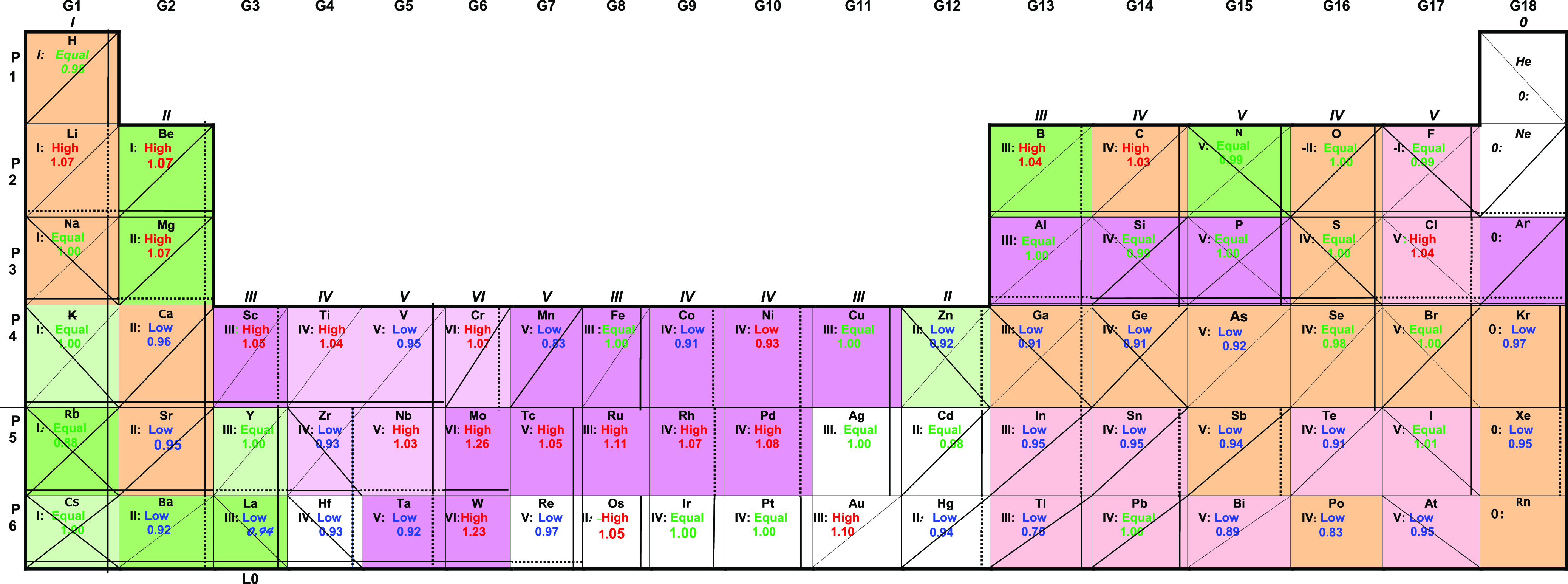
Table 1. Best Electronegativity Scales for Each Element for High Oxidation States^a.

^a

Table 2. Ratios of Pauling’s Electronegativity Scale P to the Best Representative Electronegativity Value (High Oxidation States)^a.

^a.

In Table 1, the first rank scales are shown at the beginning of the list with green letters for the most important scales and the second rank scales between parentheses for high oxidation states. The ranking for low oxidation states is given in Table S2 of the Supporting Information. The colors and marks in the cells correspond to the higher oxidation states. Ahrland⁴⁰ has also divided the Periodic Table, using in this case concepts of Pearson’s hard and soft acids and bases classification.⁴¹

As seen in Table 1, the most valid scales in the higher oxidation states are Pauling’s P and Batsanov’s B electronegativity scales, with 70 (47 in 1st rank, 23 in 2nd rank, out of range 8, and 8 not evaluated) and 63 (42 in 1st rank, 21 in 2nd rank, and out of range 23) elements, respectively. The following more valid scales are the SP (46), ARS (40), M (35), ARC (34), and PE° (27) electronegativity scales in the first and second rank levels. On the other hand, as observed in Table 1, in most of the elements the P, SP, AR, and PE° electronegativity scales are more valid, indicating that the hypothesis of equality between the free and in situ electronegativities is more common in the Periodic Table.

As seen in Table 1 for high oxidation states, the most valid scale after the best representative scale χ_DC is Batsanov’s scale with 45 elements in the first rank and 22 in the second rank (67 in total, with one element not evaluated). Batsanov’s electronegativity scale was also the second most valid scale in low oxidation states with 35 and 22 elements, respectively (57 in total, with 12 elements not evaluated) as seen in Table S2. Pauling’s electronegativity scale was the third more valid with 45 in the first rank and 21 in the second rank in high oxidation states (66 in total, with 7 elements not evaluated), and 31 in the first rank and 26 in the second rank in low oxidation states (57 in total, with 18 elements not evaluated). The following more valid scales are the G (47, 36 total elements in high and low oxidation states, respectively), SP (45, 38), A-M (29, 35), M (34, 31), ARC (32, 31), and ARS (29, 32) electronegativity scales. On the other hand, as observed in Table 1, in most of the elements, the P and B are more valid, and in second place the G and SP scales, indicating that there is a little tendency to the hypothesis of in situ electronegativity to be more common in the Periodic Table.

As a general overview of the importance of the ranking of the scales:

Sanderson’s electronegativity scale as a first or second rank scale in groups G1–G3, with the exception of La, and in groups G12 to G15, with the exception of Bi, indicates that these elements are more dependent on the polarizability in the evaluation of electronegativity. Indeed, we can explain this behavior of groups G2 and G12 to a higher influence of the polarizability of the ns² and nd¹⁰(n + 1) s² orbitals, respectively, as a consequence of having neighboring empty p or d orbitals, and p orbitals. On the other hand, the effect of the polarizability analyzed through the SP scale in periods P2 and P3 decreases in the rank of importance from the first rank in Be and Mg to the second rank in B and Al, respectively, as seen in Table 1. In this way, the effect of the normalized polarizability in the electronegativity of Be and Mg is more important in the configuration ns² than in the configuration ns²np¹ (n = 2,3).

The ARS electronegativity scale is a first rank scale from barium Ba to cerium Ce. After this element, this scale is a second rank scale, indicating that with the increment of electrons in the f orbital, the effective nuclear charge Z* and the covalent radius have a middle influence on their electronegativity.

Pauling’s electronegativity scale, in almost all the lanthanides, is a first rank scale, indicating that the high ionic resonance energy with ionic and covalent resonance structures (high nephelauxetic effect) has a higher influence on their electronegativity than only the ionic charge. This high resonance energy is associated with the orbital energy,⁴² which is increased by a strong hoping energy t₀ between the atoms,⁴³ a lower length of the bonds to the covalent radius^43,44 as happens from La³⁺ to Lu³⁺, in general, with a strong coupling between the distortion of the lattice and transfer of electrons.⁴³ On the other hand, the electronegativity elements Re to Pt are more dependent on the resonance energy as observed in Table 1 (P scale). Then, the ionic and covalent resonance structures in these elements have a higher influence on the electronegativity, as it has been explained for the lanthanides. In particular, Au³⁺ is middle dependent on the polarizability through the SP scale but not of the ionic energy of resonance, as observed in Table 1, respectively, and then the change of configuration to [Xe] 4f¹⁴ 5d⁸ in Au³⁺ produces the increment of the polarizability in the electronegativity up to the configuration [Xe] 4f¹⁴ 5d⁹ in Bi⁵⁺, as observed in Table 1 for high oxidation states.

It is also observed in Table 1 that Mulliken’s electronegativity scale is included in the first and second rank scales in the post-transition heavy metals and noble gases. This first and second ranking of Mulliken’s scale is due to the more exact evaluation of the promotion energies to the hybrid valence states of the orbitals s and p.¹⁷ This means that the hybrid configuration is more important in these elements and can be more exactly be evaluated by Mullikeńs electronegativity scale. On the contrary, the promotion energies of the hybrid orbitals for transition metals are not easy to evaluate and Mulliken’s scale is not exact for these metals.^17b,45 Also, it is observed that in the elements of a lower atomic number near Zn and Cd (G9 and G10: Co to Ag) that Pauling’s P and Allred- Rochow ARC electronegativity scales are, in general, more important. Then, as explained for the lanthanides, see above, the resonance energy and charge have a higher influence in the electronegativity. Besides, it is more possible that the orbital overlapping and formation of multiple bonds are also important, as explained above.

Concerning the actinides, we have not analyzed them in this work, because the data are scarce for the selected scales and we consider that there are few scales for doing the statistical analysis. For example, Pauling’s electronegativity scale P has only three data reported. On the other hand, Mulliken’s M, Allred Rochow’s ARS, ARC, and Allen’s A scales reported no data for the actinides. On the contrary, Batsanov’s B, Nagle’s N, and Ghosh’s GHP scales reported data for the actinides.

Ratios to the Average Value

Under the procedure for determining the best representative electronegativity values in the methodology section, we have determined the ratios of each electronegativity value to this average. The ratios to the average were ranked in low (<0.98), equal ([0.98, 1.02], and high (>1.02). Thus, these ratios of the M, P, N, SP, ARS, ARC, A, PE°, G, GHP, and B (11) electronegativity scales should have an ideal continuity in the sequence of low, equal, and high hierarchy for the elements surrounding (4) the selected element (1), so the continuity must be worth at a maximum of (4 + 1) elements X 11 scales = 55 cases for an element. This analysis serves as common and cluster analysis in the periodic network of periods and groups, as explained above. In Table 2 are shown these zones of low, equal, and high ratios for Pauling’s electronegativity scale as an example of the procedure. The other tables, S3 to S9 are given in the Supporting Information and ordered per the corresponding physicochemical property. We must remark that the jumps in periodicity in groups and periods can break the continuity of the ratios at it happens in the formation of stable configurations, the formation of multiple bonds, or the change of orbital in the electronic configuration (for example from np⁶ to np⁶(n+1) s¹).

In this way, for the higher ratios for Be and Mg in Pauling’s electronegativity scale shown in Table 2, we consider that the ionic resonance energy does not influence so much the electronegativity, but rather the effective nuclear charge and the radius have more influence as can be concluded in Table S4A (ratios of ARS electronegativity scale). It is also observed in Table 2 that Pauling’s electronegativity scale is more valid in nonmetals of low molecular weight such as N, O, F, Al, Si, P, and S because of the high ionic resonance in these elements with the influence of the variation of the bond length as explained above. On the other hand, B and C have more influence of the charge and but not so high of the variation of the bond length (first rank scale ARS in Table 1 with ratios near to 1.00 in Table S5A of Supporting Information). Besides, Pauling’s electronegativity scale is also more valid (ratio near 1.00) in Y³⁺ and Fe³⁺, and the reason would be the same as in the cases of Groups G1 (Na¹⁺, K¹⁺, Rb¹⁺, Cs¹⁺) and G11 (Cu³⁺, Ag³⁺) because of the higher ionic resonance energy (both charge and variation of the bond length). Besides, Pauling’s electronegativity scale has a ratio near to 1.00 in the low weight lanthanides, from praseodymium Pr to gadolinium Gd, and also in Lu, indicating that the resonance energy is important in these lanthanides. We consider also that the orbital overlap of the empty lanthanide f orbitals also increases the electronegativity by a covalent or π hybridization bond (correlation effects). The indirect expansion of the 4f orbitals by the higher shielding of the s orbitals due to relativistic effects⁴⁶ might increase the orbital overlapping. The lower ratios near to 0.96 in Gordy’s electronegativity scale in Table S8A (energy necessary to attract an electron from outside the atom) in almost all the lanthanides indicate that this overlap complements its electronegativity. It is also observed in Table 1 (first rank scale) and Table 2 (ratios equal 1.00) that the electronegativity values of Ir and Pt depend on the resonance energy through Pauling’s electronegativity scale P. Also, the electronegativity depends less on the environment in Zr (Zr⁴⁺) and Hf (Hf⁴⁺) because their E^°,0 values are near the curve of PE° as seen in Figure 5, see explanation of influence of chemical environment below.

Figure 5.

Dispersion of the values of P vs E°^,0 for different isoelectronic series. The scale PE° is also plotted.

Concerning Mulliken’s electronegativity scale M, it is observed in Table S3A that the ratios of electronegativity of In and Tl are lower than the average. We consider that this is due to not taking into account relativistic effects and delocalization of the electronic cloud. It is also observed in Table S3A a low value of the ratio in K, Rb, and Cs in Mulliken’s electronegativity scale because it does not take into account the higher ionic electronic resonance as Pauling’s electronegativity scale indicates as shown in Table 2. In the case of Mulliken’s electronegativity ratios, we have also considered the actualized values of ionization and affinity energy reported by Cárdenas, Ayers et al.⁴⁷ for the evaluation of Mulliken electronegativity values. We have also used the promotion energies reported by Bratsch.^17b We have found that for almost all the elements with a value in Mulliken’s electronegativity scale, the ionization potential reported by both Bratsch and Cárdenas is almost the same. The difference between both authors is in the electron affinities, mainly in G2 and noble gases. The evaluation of the electron affinities by Cárdenas was through the trend of the isoelectronic series. However, chemical perturbations in G2 and G8 can change the value of anionic promotion energy P^– and that of the electron affinity. In this way, we report the ratios of Mulliken’s electronegativity values to the best-selected electronegativity value in Table S3A and the corresponding ratios related to the energy values reported by Cárdenas in Table S3B, which have a greater difference to those of Mulliken (>0.01). Then, we have determined that in six elements, Ba, Zn, Cd, Hg, I, and Ne, Cárdenas’s electronegativity value is nearer to our proposed scale χ_DC than Mulliken’s values, see below. On the contrary, Mulliken’s values are in 11 elements nearer to our scale than Cárdenas’s values. In particular, Mulliken’s values are more congruent with our proposed scale from Kr to Rn, for example, because this scale was selected as one of the best scales in these elements. About the evaluation of the electronegativities for the transition metals, it is necessary to know the promotion energies for a specific hybridization and these values are not calculated by Cárdenas. Besides, we have also evaluated Cárdena’s et al. electronegativities in the tripartite separation and the bond force, see below, and we have found that their values are equivalent to those of Mulliken in both properties with a confidence interval of 95%. From these results, we have selected Mulliken’s electronegativity scale to determine the electronegativity average as a slightly better scale than Cárdena’s electronegativity scale.

On the other hand, we have used the rein Nagle’s N polarizability electronegativity scale¹⁸ as a probe scale. Nagle’s scale, in general, gives lower ratio values of electronegativity as shown in Table S4A (Nagle scale) because it considers that the electrons that produce the polarizability are those of the HOMO orbital. Thus, the polarizability in the transition metals in this scale is produced by the ns² electrons of the HOMO. For this reason, all the electronegativity values of the transition metals are lower than the average of the other scales as seen in Table S4A. Besides, the ratios of Nagle’s scale are between 1.0 and 1.03 in group G1 as is shown also in this table, indicating that its polarizability in this group is important to determine the electronegativity. Also, Nagle’s electronegativity scale has almost a constant ratio (0.88–0.93) to the average in the lanthanides from Pr to Gd. As it has already been remarked, Pauling’s electronegativity scale has a ratio near to 1 in these elements. This indicates that the ionic resonance energy improves the electronegativity in the lanthanides and their polarizability predicts a low electronegativity.

In order to analyze the normalization of the polarizability by the corresponding values of the isoelectronic noble gas of the same period, we have analyzed Sanderson’s electronegativity scale. We have found in this scale that the ratios of the polarizability weighted by the atomic volume have critical importance in H, C, O, Ne, Ar, Br, Sr, from Cd to Te and Pb, as shown in Table S4B of the Supporting Information. Then, as explained by the absolute values, see above, the effect of distortion of the electronic cloud (in this case, the rigidity of the electronic cloud) affects substantially the electronegativity of In, Sn, Sb, and Te, for example, more than the resonance energy given by Pauling’s scale (Table 2) or the energy associated with the hybridization given by Mulliken’s scale (Table S3A).

In this way, Sanderson’s scale is a 1st rank scale with both a difference of electronegativity not greater than 0.6 to the average and ratios between 0.98 and 1.02 in a wider zone of the Periodic Table. This results in 25 times in high oxidation states and 21 times in first ranking low oxidation states and being the 4th best scale after the B, P, and G scales. Nagle’s electronegativity scale has only 14 and 15 in the first ranking, respectively. Therefore, the normalization of the polarizability to that of the noble gas of the same period decreases the alteration of electronegativity (as happened in Nagle’s electronegativity scale) by a change of period as Sanderson has remarked,¹³ and then the validity of the values goes up. In particular, the configurations ns² (n = 2, 3 = Be, Mg) with their neighboring empty p orbitals produce higher resonance energy with lower polarizability (higher predicted electronegativity than the average) as seen in Tables 2 and S4A (Nagle scale), respectively. Concerning the reduction potential, the elements Be⁰ and Mg⁰, with configurations 2s² and 3s² have a maximum of the reduction potential E^°,0 in their isoelectronic series as observed in Figure S15 of the Supporting Information.²⁹ Besides, the corresponding ions of Be²⁺ and Mg²⁺ with configuration 1s² and 2p⁶, respectively, have a trend of a higher reduction potential E^°,0 with a higher atomic number in their respective isoelectronic series as seen also in Figure S15. We would expect then a higher electronegativity for Be and Mg. However, the average electronegativity of Be and Mg is lower because their full s² orbitals and empty p orbitals have a similar volume. This produces a lower augmentation in the attraction of the electrons from orbital p. The ratios of Sanderson’s electronegativity scale SP near and lower to 1.00 for Be and Mg (Table S4B) clarifies that the volume of both orbitals s and p has an influence on the electronegativity at opposite to happens with the rein Nagle polarizability scale (Table S4A), which also predicts a higher electronegativity. This occurs by the normalization to the atomic volume of the noble gas of the corresponding period. On the other hand, the ns² configuration (n ≥ 4: Ca, Sr, Ba) with the neighboring d orbitals has a lower effect of the ionic resonance energy on the electronegativity than the configuration ns¹ as seen in Table 2. Then, the calculated average electronegativity of Ca and Sr is higher than Pauling’s electronegativity scale prediction. This higher attraction of electrons is due to a lower expansion of the volume from the full ns² to the empty nd, whose volume is lower.²⁰ This produces a lower attraction of electrons by the nd orbitals. We can say then that the ns² orbital, more in Ca and Sr, is a potential well influenced more for the polarizability and charge as seen in Table S4B (SP scale) and Table S5A (ARS scale), respectively. Besides, Sanderson’s electronegativity scale is dependent on the high or low polarizability of the elements. For this reason, groups 3 and 4 show a predicted high value of the electronegativity as a consequence of lower polarizability, even more than the average as seen in Table S4B (SP scale), as a consequence of the higher electronic density than group G2.

Concerning the ARS electronegativity scale, this scale is more exact in the configuration ns² as seen in Table S5A, which implies that the effective charge Z* and the covalent radius are more valid to evaluate the electronegativity in this configuration. The same applies from boron B to O, even F (but in this case as second rank scale). On the other hand, the ARS electronegativity scale can also be used as a probe scale. For example, the higher importance of the relativistic effects from Pt to Pb produces a ratio of approximately between 0.63 and 0.67 (Table S5A: ARS scale) where the polarizability due to the delocalization of the electronic cloud (Table S4B: SP scale) to the orbital 6p is more important. Also, the importance of other factors than the nuclear charge in the increase of the electronegativity in the noble gases produces a decrease of the ratio from He (1.37) to Rn (0.74) in the ARS scale. The fall of the electronic cloud polarizability for noble gases with the increment of Z (Table S3B: SP scale), which produces both a lower radius with respect to the near elements of the period⁴⁸ and a higher total energy which induces a higher penetration of the orbitals causes this increase of electronegativity.

Equally, the ARC electronegativity scale can also be used as a probe scale when the ratio is low as this scale indicates a higher influence of the nuclear charge (higher effective nuclear charge Z*). Thus, a low value of the ARC scale indicates that the orbital overlap has exceeded the ionic resonance attraction, and in this way, this effect is higher in Group 6: Cr and Mo (multiple bonds) as seen in Table S5B (Low ratios in the ARC scale). In this context, it is convenient to compare Table S5B with the division of the Periodic Table made by Ahrland.⁴⁰

Regarding Allen’s electronegativity scale A or A-M, this scale does not consider the sequence of electronegativity for orbitals s > p > d, and p post-transition < p nonmetal elements. For this reason, the ratios of electronegativity are lower in the post-transition heavy metals, as seen in Table S6A (allen scale: ratio = low in P4 to P6). Nevertheless, Sproul³⁴ has found that Allen’s electronegativity scale is one of the more valid scales for analyzing the tripartite separation in 311 ionic, covalent, and metallic compounds, as explained above. Indeed, other scales can give almost the same results for the tripartite separation^34a of type of bonds as it happens with Nagle’s and Batsanov’s electronegativity scales, Batsanov’s scale being the best. On the other hand, we have evaluated the Tables of Electronegativity of Rahm, Hoffmann, et al.,⁴⁹ and Politzer⁵⁰ by our methodology (Table S6B Rahm, Hoff-A and Table S6C POL-A respectively). Indeed, the Politzer methodology uses the DFT analysis and the average energy of the orbitals as Allen proposes. We have concluded that their values are similar to Allen’s electronegativity values. Indeed, the values of Hoffman extend the average orbital energy Allen’s concept to the evaluation of transition metals and lanthanides. Again, as it happens to Allen’s, Politzer’s and Hoffman’s electronegativity scales (even Nagle’s scale) have a low value in transition metals and post-transition elements under our electronegativity scale (Table S3B: Nagle scale, Table S6B: Rahm, Hoff-A scale and Table S6C: POL-A scale). The same occurs when we relate their ratios to those of Pauling’s electronegativity scale (Table 2). We consider that the electronegativity is also caused by the overlap of the electronic orbitals (considered as waves) or by the formation of double and triple bonds. These phenomena add a term to the nuclear charge, electronic correlation effects, and attraction of electrons terms evaluated by the average energy of one electron.⁴⁹ We consider that the configurational energy CE (electronegativity) is underestimated, because of, as explained above, not taking into account the orbital overlap as it is taken into account in the situ hypothesis, see above. For example, the s orbitals of the Ti²⁺ ion are less occupied in the bond of the compound TiCl₂, and then the d orbitals are more occupied.²⁹ The higher occupation of the d orbital increases the CE (electronegativity). We consider that the reference zero of the energy of attraction at the outside of the atom and higher energy of attraction as the electron is nearer the atom in the analysis by the configurational energy CE is equivalent to the higher ionization and affinities energies. In this context, we consider that the filling and overlapping of the s orbitals in the transition elements and degree of penetration of the s orbitals is underestimated. On the other hand, the higher values of the ratios in the transition elements as seen in Table S8B of Gordy’s electronegativity scale indicate that the s orbital is more occupied, and overlap more with the other element, and then the electronegativity is higher than those predicted by the splitting of the electrons in the s and d orbitals proposed by Mann.^24a We also must clarify that Allen’s methodology considers the atom in its ground state, without taking into account the bond overlap as in the situ hypothesis, which increases the electronegativity as in Mulliken’s methodology. As an additional point to remark, Politzer’s electronegativity scale POL-A gives practically the same values of the best-selected values in O, S, F, and Cl, at the difference from the A, Rahm-Hoff-A and χ_a scales as seen in Table S6B.

Concerning the PE° electronegativity scale, its advantage is that the reduction potential E^°,0 is determined with four digits of precision, and also, all the oxidation states can be measured (see Methodology Section where the PE° scale is analyzed). If we define the electronegativity as an average of the attraction and holding of electrons in an oxidation state to the neutral elements, the definition of E^°,0 has a similar trend.²⁹ This equivalence would explain the fact that different oxidation states have the same electronegativity and the similitude of the electronegativity of a free atom electronegativity with the electronegativity in an oxidation state. As a consequence, the PE° scale is based on the macroscopic power to attract electrons based on both Pauling’s scale (through the resonance energy) and lesser dependence on the chemical environment; it should be tested in order to find if this scale is more valid in the evaluation of a macroscopic electronegativity not dependent on the chemical environment. Indeed, we can use this characteristic to use the PE° electronegativity scale as a probe scale for the evaluation of the dispersion of the experimental values of P versus E^°,0: a higher dispersion indicates a higher influence of the chemical environment. This is indicated by ratios lower and higher than 1 in Table S7. On the other hand, a ratio near 1.00 indicates that the chemical environment does not have a high influence in the electronegativity. In this way, we can observe that there is a slight increase of the influence of the chemical environment in the electronegativity from the element Ce up to Dy to the elements Ho up to Lu as seen in Table S7 (PE° scale) because the ratios decrease in the last elements. On the other hand, the higher ratios in this table for most of the transitions metals indicate a higher predicted electronegativity by the reduction potential E^°,0.²⁹ In principle, the transition metals can form complexes and the higher ratios indicate that experimental bonds with the ligands are less ionic than the PE° scale predicts. Besides, the lower ratios in Group 3 indicate that the electronegativity is higher than that predicted by PE° and then the bonds are more covalent with the ligands. Zones with ratios near 1, which indicate that the chemical environment does not have appreciable influence, are near fluor F, rubidium Rb, and gallium Ga as seen in Table S7 (compare also Table 1). Also, these values near 1 indicate that the ionic resonance energy of the bond is important in the determination of the electronegativity.

We have also used Gordy’s electronegativity scale G²⁷ in the ranking of scales. This scale, in particular, is associated with the energy to translate a positive charge to the HOMO (the negative charge only changes the sign of the energy). The supposition of considering the external electrons of the HOMO as the charges to be translated from outside produce that this scale is a thumb scale. Also, this scale has no valid values for the transition elements from G6 to G10 as seen in Figure S9B and Table S8A with a gradual increase of the inexactitude. Therefore, we have not used this scale in the evaluation of the average, but it was evaluated in the ranking. Unexpectedly, this scale is the 3rd ranked scale, after the Batsanov’s and Pauling’s electronegativity scales. We consider that the energy factors (configurational energy, ionization and affinity energy, resonance energy) which influence the electronegativity are averaged in the ratio (n + 1) e/R_cov, n being the number of external HOMO electrons, see above. In other words, the overall energy of attraction is averaged on this scale. As seen in Table S7A, this scale is, in general, more valid from group G1 to group G5 than in the other zones of the Periodic Table because the number of valence electrons is almost the nuclear effective charge Z* calculated by Slater’s shield constants. The same happens in the nonmetals of period P2. However, Gordy’s scale predicts a high electronegativity in the transition elements from G6 to G10 because it does not consider, for example, the ligand field splitting of the valence electrons in orbital d, which diminishes the number of electrons of valence. Besides, Gordy’s scale predicts a lower electronegativity than the average in groups 11 and 12 and in the high post-transition elements, because its formula has a low slope (0.31), indicating a low increase of the electronegativity with the increment of valence electrons in these elements or that the number of valence electrons to be considered must be higher. This is the reason that the ratios go up from a low value in G11 to a high value in G17. On the other hand, we have considered that the lanthanides have three electrons as the short Periodic Table suggests and we have found that this scale is a first rank scale for most of the lanthanides. Then, we consider that although this scale is a thumb scale, as explained above, this scale is an average of the behavior of the main transition elements in periods 1–3, low-weight-transition elements and lanthanides. Also, if we compare Gordy’s and Allen’s electronegativity methodologies, there is a contradiction between them, because a higher occupancy of both s and d orbitals in the transitions element causes a higher electronegativity in Gordy’s methodology. On the contrary, higher occupancy of the d orbitals instead of the s orbital produces a higher electronegativity in Allen’s methodology. That is the reason that Gordy’s electronegativity ratios in Table S7A are higher than the ratios of Allen’s electronegativity scale. Then, the penetration or overlap of the s orbitals also influences the evaluation of the electronegativity, and Allen’s methodology does not take into account its influence in the increase of electronegativity. That is the reason that the electronegativity of chromium Cr in Allen’s scales is 1.65, Gordy’s electronegativity value is 2.06, and the average in the low oxidation state is 1.73 with an occupancy of s (x = 1.779) and d (1 – x = 4.221). It is a higher difference of electronegativity in this element because there is a higher occupancy of an s orbital and then the electronegativity is higher in Gordy’s scale, but the electronegativity in Allen’s scale is lower.

Besides, we have evaluated the ratios of Ghosh’s scale of electronegativity GHP related to Gordy’s electronegativity scale^4b (Gordy’s electronegativity scale), but with the Slater radius. Thus, we have found that the values correspond to the equal ratio in half of the nonmetals (groups G13–G17) excepting B, F, Al, P, Ga, Ge, Br, In, Sb. Te, Pb, Tl, Po, and At, as seen in Table S8B (GHP scale). However, this scale in all other zones of the Periodic Table is only an equal ratio scale in the elements Nb and Cd. We consider that in Nb and Cd the free atom electronegativity hypothesis, following this scale, is valid and the ground state has influence on electronegativity. This is different to the qualification of the element Ga, in which the PE° scale is more valid and then there is a low influence of the chemical environment, but there are internal factors associated with the bond between atoms such as the resonance energy or hybridization that increase electronegativity with respect to that of the free atom electronegativity (GHP scale), as seen in Table 1. In this context, Ghosh has also determined the electronegativity values of an Allred Rochow scale ARGH, relative to the electric force, which considers Slater’s radius of the isolated atom in the ground state and an effective charge whose values are between Slater’s and Clementi-Raymondi’s effective charges.⁵¹ It was necessary to adjust the Ghosh values of force to Pauling’s units scale ARGHP and the correlation was ARGHP = 1.40737 10¹⁶ ARGH^0.27/((2.74832 10⁵⁹)^0.27 + ARGH^0.27) with R² = 0.82. Both electronegativity scales ARGHP and GHP (Tables S5C and S8B, respectively) have similar or slightly higher ratios, in general, to Pauling’s and Batsanov’s electronegativity scales (Tables 2 and S9) in groups G1 and G2, periods P2 and P3, and the post-transition elements. On the contrary, Allen’s electronegativity scale (Table S6A) has lower ratios, in general, in groups G1 and G2, periods P1 and P2, and in the post-transition elements. In this way, there is a contradiction because the ground scales ARGHP and GHP predict higher or equal electronegativities than the in situ Pauling’s and Batsanov’s electronegativity scales, and the ground state Allen’s electronegativity values are lower. We remark again that this is because Allen’s electronegativity scale does not consider overlap and/or higher penetration of orbitals s and p. As a note for the ARGHP scale, we have found that this scale is a first or second rank scale in the noble gases, except in He, indicating that the isolated atom ground state (charge and radius) has a higher influence on the electronegativity of these elements.

Besides, we propose a new scale related to the ARS and G scales, named GORS. In this scale, the number of electrons was changed by an effective nuclear charge Z* and the element F/GORS = 0.50 Z*/R_cov + 0.744 was taken as reference. This scale predicts higher electronegativity values as seen in Table S8C (GORS scale) because of its higher slope (0.50) than that (0.31) of Gordy’s G electronegativity scale. In this way, the GORS electronegativity scale is a first scale rank in the elements N, Mo, Tc, W, Os, Ir, and Hg (less effect in He, C, O, F, Nb, Ru, Rh, Re, Tl, and Pb). We consider that in these elements the value of the radius has a higher influence on the electronegativity.

Evaluation of the Periodicity of La and Lu through the Absolute Values and Ratios of Electronegativity to the Electronegativity Scale χ_DC

We have also analyzed statistically the periodicity among⁵² Ba, (Sc) Y, La, Lu, and Hf using all the before-mentioned scales, as it is more explained in Section S-7 of the Supporting Information. Then, (1) La has continuity in the absolute value and ratios of electronegativity with yttrium Y and scandium Sc under Pauling’s electronegativity scale, the most valid scale for La along with Gordy’s electronegativity scale (relationship of La with G3), (2) the electronegativity ratio of La has continuity with Ba in absolute values but not in the ratio to the electronegativity scale χ_DC; then, the physicochemical properties indicate a similitude of La and G2 but not the proportion of influence of the physicochemical property on the total electronegativity given by the ratios. On the other hand, La and cerium Ce have continuity in absolute value and ratios of electronegativity under all the scales of electronegativity (relationship of La with G2 and lanthanides), (3) Lu is considered as the last lanthanide because it has almost always continuity with the values of the precedent lanthanides, but it does not have a strong relationship with Ba or Y (less relationship of Lu with G2 and G3), (4) La and Lu have a light continuity (2 and 3 scales, respectively) in their electronegativity ratios to Hf. On the contrary, the absolute values indicate a higher similarity from La and Lu to Hf (7 and 8 scales, respectively), which means a similar power to attract or hold electrons in a specific electronegativity scale related to a specific physicochemical property (relationship of La and Lu with G4). As a summary, La has continuity with G3 and the lanthanides, and its relationship with G2 and Hf depends on the way the relationship is made. Indeed, the higher relationship of Ba, Sc, Y, La to Ce, and Lu to Hf can also be observed by the corresponding Frost and reduction potential diagrams as seen in Figures S16A/B.

Analysis of the Physicochemical Characteristics of the Electronegativity

In the selection of the best values of electronegativity for the elements, a theoretical analysis applied to the Periodic Table must also be undertaken. In this way, a lower band gap (hardness η^15d,32) indicates that the acceptation of electrons is higher (higher reduction), and the electronegativity χ called the negative of chemical potential −μa^,15c is higher. The increase of electronegativity with a decrease of the band gap is due to the inverse relationship of the hardness η (half of the bandgap) to the electronegativity (see Appendix S-A in the Supporting Information for the deduction) considering that the reference of energy is outside the atom.b

5

In this way, the higher band gap in low spin complexes of transition metals (higher ligand field stabilization energy^15a Δ₀ in units of⁵³ 10 Dq) can produce a lower electronegativity (with exceptions).⁵⁴ Indeed, the relation of the hardness η (band gap) to the Coulomb integral⁵⁵J (electrostatic) repulsion and the exchange integral K (quantum mechanics repulsion produced by the higher proximity of an electron and its interchange)⁵⁵ is (for a singlet or triplet)⁵⁶

6

This equation is obtained by the DFT Kohn Sham Theory.^15d The implied phenomenon occurs when a new electron is added in the LUMO and this electron is repelled by the electron in the HOMO, which also is a valence electron. Thus, Vg., a higher electronegativity, is obtained with a lower value of J or/and +K. Hence, we can calculate the influence of the correlation effects (J + K) by the difference of the electronegativity obtained by Mulliken’s model M minus the electronegativity obtained by electrostatic models such as the ARS or Boyd’s electronegativity χ_B models.⁵⁷ In the case of the ARS electronegativity model, we equate the ionization potential EI_v to the F_elec (Newtons) times the radius of the element or ion R (meter) for an electron in order to have units of volts

7

From Allred Rochow for²¹

8

EI_v in eV and e is the conversion factor of Joules to eV.

From eqs 6 and 7

9

In this way, Mulliken’s electronegativity χ_Μ (eV) is

10

11

In Pauling Units (M and ARS), we obtain through the relation of Allred Rochow,²² see above, the values of the scale ARS, and through Bratsch’s relation^17b

12

The following equation

13

and using only the equation of Bratsch considering the equivalence of the M and ARS scales for the evaluation of the band gap, in which J–K (eV) has negative values corresponding to the triplet

14

In this way, concerning the values of M and ARS for group G1, where M and ARS are first rank electronegativity scales for almost all the elements, values of the gap 2η with a ratio of 6 to the experimental value are obtained by eq 13. Besides, negative values of (J–K) obtained for group G1 by eq 14 because of adding an electron results in a paired electron, which is a triplet. On the contrary, in group G2, positive values of (J + K) are obtained by eq 14 because the addition of an electron in the proximal orbitals p or d results in a singlet, with a higher energy of repulsion than a triplet.

Besides, following the meaning of Clebsch–Gordan or vector coupling coefficients, a lesser similitude of the orbitals HOMO and LUMO produces a lesser value of these coefficients⁵⁵ and then a higher electronegativity. In this way, smaller polarizability, lower relaxation phenomena^56b of the HOMO and the LUMO produce an increase of electronegativity. On the other hand, as observed by Gázquez,⁵⁸ when the relaxation of the orbitals is included in the evaluation of the electronegativity, the electronegativity equation resembles that of Gordy’s more.⁵⁸

15

where q is the increase of the positive or negative charge and ν_i is the principal quantum number of the hydrogenic orbital. In this way, as seen in eq 15, when the relaxation of orbitals is important the radius r and the principal quantum number ν are important to evaluate the electronegativity. In the second term, the added positive charge q increases the electronegativity because of the Coulombic charge force attraction and through the concomitant decrease of the radius r. On the contrary, electronegativity goes down with the augmentation of the negative charge q in the second term of this equation, which is attenuated by the increase of the radius as a consequence, for example, in transition metals, of the nephelauxetic effect. This is, for example, observed in Figure S15, where an increase of the negative oxidation state decreases the value of E^°,0 (electronegativity) for the isoelectronic series F^1–, O^2–, and N^3–. In the third term, the electronegativity increases with a positive or negative charge because of the square of q and is associated with the nephelauxetic effect in the transition metals. This augmentation is attenuated by a higher value of the principal quantum number ν. Besides, by the DFT Kohn Sham Theory,^15c,59 a diminution in the kinetic energy of the electrons or/and a negative variation in the repulsion of the electrons with an augmentation of the charge density can increase the electronegativity. This can be deduced from eqs 16 and 17, as in the case of tungsten, which forms triple bonds.

16

17

where μ is the chemical potential, v(r) is the one-electron external potential, T[ρ] is the electronic kinetic energy functional, and V_ee[ρ] is the electron–electron repulsion functional. Considering the validity of the Kohn Sham equation for an isoelectronic series, we have found that E^°,0 versus Z explains the same behavior found by the DFT theory: the rise of the reduction potential E^°,0 (electronegativity χ) from N^3– to C^4– in E^°,0 with the increase of the negative charge as seen in Figure S15.

Also, we have considered the following factors to select the best values of electronegativity: the orbital shielding, the polarizability of the electronic cloud, the similarity of the band gap and low energy of the LUMO, the relativistic effects with contraction of the s orbital and expansion of the d orbital, the higher penetration of the s orbitals which produces a higher electronegativity, the orbital overlapping, the electronegativity alternation of the elements among the periods, the formation of multiple bonds, the higher bond length, the silicon rule, π backbonding, the lattice energy with the Madelung constant, Racah’s constant, the spin of the orbital, the inaccuracy of the metal bond energy, the polarizability of the electronic cloud which includes the dispersion of the electronic charge in the unoccupied neighboring orbitals, and so on. These factors are explained in the Supporting Information, Section S-8.

Best Representative Values of Electronegativity

In Table 3 are given the best representative values of electronegativity for the elements named the χ_DC electronegativity scale and plotted in Figure 1. The graphics of low and high oxidation states of the average values versus the atomic number and for low oxidation states versus groups are plotted in Section S-2.10 of the Supporting Information. The criteria used to determine the best representative value of electronegativity allow obtaining the electronegativity values with an exactitude of hundredths. The selection of the representative value also considers the periodicity of the ratios in the neighboring elements in columns and rows and the periodicity of electronegativity in similar electronic configurations and periods, for example, in the noble gases as seen in Figure S22 of the Supporting Information. The procedure for selecting the best representative values is given in the methodology section. On the other hand, we have used similar (and more common) oxidation states in a group in order to compare the electronegativity between periods. In this way, for group G8, the common oxidation states of Fe (II, III) determined the analyzed oxidation states in Ru and Os. Nevertheless, we have added affordable electronegativity values of the groups G8 (Ru and Os) and G9 (Co and Rh) of other oxidation states not so common, which have a difference of 2 to the other oxidation states. They are indicated in blue in Table 3. On the other hand, we consider that the difference of |χ_{highoxidationstate} – χ_{lowoxidationstate}| < 0.06 indicates that the electronegativity of the free atom is similar to the electronegativity in situ, as happens in 46 elements, for example, W, Cu, Au, Ga, Ge, and As, as observed in Table 3, and then both hypotheses give the same results. Besides, a difference between both hypotheses (>0.06) is found only in 14 elements: Sc, Y, La (G3), Eu, Zr, Cr, Mo, Mn, [Ni, Tl, Pb: in these three is the highest difference], Te, Po, and At.

Table 3. Values of Díaz-Campero’s Electronegativity Scale χ_DC.

Figure 1.

Trends of the best-selected values of electronegativity for the 86 elements ordered in Periods and Groups (a) considering all the groups, (b) without considering groups 3–12 (variation of orbitals s and p).

Periodicity

Periodicity in Groups and Rows

Having determined the best representative values of electronegativity, the next step was to find the periodicity of these values. In this way, the values of the electronegativity in group 12 alternate in Table 1 (high, low, high) unlike the electronegativity values of Pauling, which increase sequentially (Figure S1B in the Supporting Information).¹⁶ Concerning the noble gases, the electronegativity scales ARS, ARC, A-M, PE°, G, and GHP (see Section S-2 of the Supporting Information) are consistent with the requirement of Allen and Huheey^1b,60 that the noble gas electronegativities are higher than those of the respective halogens. On the contrary, Pauling’s P, Mulliken’s M, Sanderson’s, and the Batsanov’s scales predict that their values can be not higher than those of the halogens,^{16,17b,28,60a} (see Section S-2 of the Supporting Information). Concerning also the scale χ_DC, we have found that the electronegativity values of the noble gases are higher than the those of the halogens, supporting the asseveration of Allen and Huheey.

In the evaluation of the sequence of electronegativity in the lanthanides, it is observed in Figure S17 that Eu has more instability in oxidation state 3+ (ΔG_0,Ox°/F more positive = it has more tendency to be reduced) than Sm and Gd; this produces a higher electronegativity than the periodicity predicts, as also observed in Table 1. On the other hand, Yb³⁺ has a similar ΔG_0,Ox°/F value as Tm³⁺ and Lu³⁺. This indicates that Yb has an electronegativity similar to Tm and Lu as also shown in Table 1. On the other hand, in Figure S18 it is seen that the reduction potential E°^,0 of the cations Eu²⁺ and Yb²⁺ is less than those of the cations Eu³⁺ and Yb³⁺, respectively, which is correlated to the same relation in electronegativity. Importantly, we can make these comparisons only in Eu because the PE° scale is the most important electronegativity scale in this element and second rank scale in Yb as shown in Table 1.

In Figure 1, the continuity of the slope in several zones of the periodic table is remarkable although the average is made by each particular element. In particular, the changes of slopes and the jumps in electronegativity indicate the appearance of a stable electronic configuration or a special chemical property, such as the formation of multiple bonds or the increase of the overlap of the wave orbitals. These changes of slopes or jumps are more important in this averaged scale for specifying the apparition of a physicochemical property because there are scales such as the ARS and Allen’s scales, which have few of these changes of slope or jumps in electronegativity as observed Section S-2 and then soften these perturbations in the periodicity.

As explained above, the shifts of the linear periodicity of the electronegativity scales indicate the appearance of a new physicochemical property. For example, the decrease of the slope of electronegativity in V³⁺ to Mn²⁺ in low oxidation states (Figure S12B in the Supporting Information) to about V⁵⁺–Mn⁵⁺ in high oxidation states (Figure 1) is due to the easiness of obtaining the configuration [Ar] 4d⁵ in Mn²⁺ (a stable configuration) from the configuration [Ar] 3d⁵ 4s² of Mn. This produces a lesser electronegativity in Mn²⁺ in order to get the configuration d⁵. Besides, the configuration 4d² of Mn⁵⁺ allows a higher electronegativity because of the higher configurational energy of the d orbitals^24a and the higher ionic charge. Mn⁵⁺ also has a higher variation of electronegativity with respect to Mn²⁺ (1.87 vs 1.72, respectively). This indicates that in situ electronegativity is more valid and then the electronegativity depends on the oxidation state. The same phenomenon happens in the higher decrement of electronegativity between Co³⁺ and Ni²⁺ (Figure S12B in the Supporting Information) in relation to Co⁴⁺–Ni⁴⁺(Figure 1) because of the higher stability of the configuration [Ar] nd⁸ (square planar)^15a of Ni²⁺ to the configuration [Ar] nd⁶ (octahedral) of Ni⁴⁺. Then, Ni is more prone to lose the electrons to get the oxidation state 2+. On the other hand, the higher value of the electronegativity of tungsten W and molybdenum Mo than the predicted periodicity as seen also in Figure 1a is assigned to the easiness to build multiple bonds of these elements. On the other hand, the sharp drop of the electronegativity in group groups 11 and 12 of Periods 4 and 5 indicates that the configurations (n – 1)d¹⁰ns¹ and (n – 1)d¹⁰ns², respectively, tend to get the oxidation states 1+ (low oxidation states) and 3+ (high oxidation states) and 2+ with the stable configurations (n – 1)d⁸ and (n – 1)d¹⁰, respectively. For this reason, its electronegativity is lower. This decrement of electronegativity does not happen in Au (2.3 in low and high oxidation states) of G11 and Period 6, with a higher electronegativity than Pt (2.24 low oxidation state and 2.28 in high oxidation state) as seen in Figure 1a because of the higher influence of the polarizability, as explained above.

Regarding the post-transition elements, the electronegativity scale PE° is a first rank scale in Period P4 and groups G12, G13, and G14 as observed in Table 1. Then, the reduction potential referenced to the oxidation state of the element E₀° has more influence on electronegativity. In the same fashion, the reduction potential E₀° of the isoelectronic series 3d¹⁰ has a similar linear increasing trend with the ions Zn²⁺, Ga³⁺, and Ge⁴⁺ as shown in Figure S19 of the Supporting Information. Thus, we can say that the reduction potential E₀° is linearly associated with the electronegativity in these elements.

About periods P5 and P6, there is a transition of the influence of the polarizability (Sanderson’s scales) from groups G12 to G15, as explained above, to the influence of the energy of the hybrid states (M scale) in groups G16 to G17 as seen in Table 1. The possible explanation is that the increase of the electronegativity measured by the rigidity of the electronic cloud in groups G12 to G15 is higher than that of group G16 to G17, where the ionization and affinity energies are more important. Also, there is almost a linear trend of increase of electronegativity from the oxidation state 2+ of group G12 to the groups G13 and G15 with oxidations states 3+ and 4+, respectively, for all the periods, with the exception of period P6, as shown in Figure 1b. In the same fashion, in the case of the isoelectronic series 4d¹⁰ in period P5 shown in Figure S20, the reduction potential E₀° has a linear increase for Cd²⁺, In³⁺, Sn⁴⁺, Sb⁵⁺, and Te⁶⁺ with electronegativity of the groups G12 to G16 in period P5 as seen in Figure 1a. In this case, Sanderson’s electronegativity scale SP (polarizability) is a 1st rank scale that influences this linear behavior but not the PE° scale (reduction potential without the influence of the chemical environment). In period P6, there is a sink of the slope of electronegativity from group G14 to group G15 as seen in Figure 1, opposite to the constancy of the reduction potential E₀° in configurations 5d¹⁰, as seen in Figure S21 of the Supporting Information. We consider that group G15 in period P6 (Bi⁵⁺) has a stable configuration 5d¹⁰ 6s² 6p³ with orbitals p half-filled and then has a lower electronegativity (less tendency to attract or hold electrons). This is corroborated by the ionization, affinity, and promotion energies (Mulliken)^17b in Period P6, which decrease fast from groups G17 (At) to G15 (Bi) and then they increase in groups G14 (Pb) to again decrease from group G14 to G13 (Tl). This behavior happens between Pb and Bi in Period 6. On the contrary, this does not happen between Ge and As, and Sn and Sb; this explains the linearity in periods P4 and P6. In principle, the sequences of electronegativity ratios for the periods P4 and P5 for Ge⁴⁺ in its first rank PE° scale (Table S7) are sequentially congruent.

In general, the variation of the continuity of the slope of electronegativity in Figure 1a might be due to inherent physicochemical characteristics, for example, by the electronic configuration. In this order of ideas, a sink of electronegativity is found from period P1 to period P2 in group 1 from H to Li because group G1 does not have p orbitals, as observed in Figure 1a, with a subsequent higher slope in electronegativity in Period 2. Thus, this is the reason for the jump of electronegativity between He and Ne as seen in Figure S22 of the Supporting Information Section S-11. On the other hand, the scandide (d orbitals) and lanthanide (f orbitals) contractions⁶¹ produce a lower slope in the electronegativity versus group number in periods P4–P6 than in periods P2–P3 as seen in Figure 1. Concerning the scandide and lanthanide contractions, it has been considered that the p orbitals might have a similar phenomenon.⁶¹ In this way, if we analyze the elements of periods P1 to P3, we can speak of a “Lithide” contraction (orbitals p) between periods P2 and P3 because of the lower increment of the radius than in period 1. Indeed, the augmentation of the effective nuclear charge Z* is lower in period P4 than in periods P2 and P3. This behavior indicates that the slope of the electronegativity is higher in periods 2 and 3 versus Z than in period 4.

Besides, concerning the periodicity of La and Lu in the scale χ_DC with the lanthanides and groups and periods near them, continuity of the trend from La(III, G3) to Hf, Ta, and W is found as seen in Figure 1a. Lu also follows the trend of Hf, Ta, W as seen in Figure S12C. Then, we can say that La, Lu, and Hf have periodicity among them in the scale χ_DC and that the lanthanides are from La to Lu, which increase their electronegativity until a value in Lu that follows the trend of Hf, Ta, and W as seen also in Figure 1a and Figure S12C of the Supporting Information. It is also seen in these figures that in La converges three tendencies; the tendency of G3 (Sc, Y, La), the tendency of period P6 (Cs, Ba, Hf, Ta, W), and the tendency of lanthanides (Ce to Lu); as a consequence La belongs to these three groups. On the other hand, two tendencies converge in Lu: P6 and lanthanides, and then Lu belong to these groups. Then, La has the trend of G3, P6 (short Periodic Table), and lanthanides and belongs to them. On the other hand, Lu has the trend of the period P6 (short Periodic Table) and lanthanides. Also, Hf and Ba only belong to the tendency of period P6 as seen in Figure 1. The other lanthanides do not tend to belong to period P6 because they form an internal bridge between G2 and G3 to give to them continuity in the electronegativity values, but they do not follow the tendency of period P6 (short Periodic Table).

If we cut more the extension of the Periodic Table, eliminating the transition elements and the lanthanides, that is, eliminating the sequence of elements with orbitals d and f, it is observed that Groups G2 and G13 has a jump as seen in Figure S1b. This jump is similar in periods P4 and P5, and it is a higher in period P6 as seen in Figure S1b, with a higher difference among periods P4 to P6 in groups G13 and G14, to reach a zone of not a great difference of electronegativity from group G15 to group G17 and to be separated again in G18, the noble gases.

Evaluation of the Electronegativity Scales (χ_DC)

As explained above, the electronegativity scales are associated with specific physicochemical properties, and the evaluation through another physicochemical property gives the ranking to this physicochemical property. In this manner, we consider three ways to evaluate the electronegativity scales: (1) periodicity, (2) chemical bonds, and (3) force of bond attraction as physical property.

Higher Influence on Electronegativity of an Element (Chemical Periodicity)

The evaluation of the chemical periodicity is through the ranking with respect to the best representative value of the scale χ_DC through differences of the absolute values and ratios of electronegativity. As explained above, this scale is considered the best concerning the chemical periodicity because it weighs the more important factors through the average, but this scale cannot be the best in a specific element, as explained above. The following best individual scales for low oxidation states with a confidence interval of 95% of similarity in chemical periodicity are Batsanov’s B, Pauling’s P, Sanderson’s SP, and Mulliken’s M electronegativity scales. The scales in the third place in the ranking are Gordy’s G, Allen’s A-M, ARC, Ghosh’s GHP, and ARS electronegativity scales. In a fourth section of ranking are Nagle’s N and the PE° electronegativity scales. About the high oxidation states with the same confidence interval of 95%, Batsanov’s B, Pauling’s P, Sanderson’s SP, and Mulliken’s M electronegativity scales are in the second section of the ranking. In the third section of the ranking are Gordy’s G and Nagle’s N electronegativity scales, and in the fourth section the ARS, PE°, Allen’s A-M, and Ghosh’s GHP electronegativity scales. The second ranking of Sanderson’s SP electronegativity scale is due to the low number of elements evaluated (54) with a high number in the first and the second ranking in low and high oxidation states, 38 and 45, respectively. This encourages the experimental evaluation of the electronegativity of the remaining elements. The same applies for the Mulliken electronegativity scale.

Tripartite Separation

We must clarify that the lines of separation in the van Arkel–Ketelaar triangle of Pauling’s electronegativity scale take into account the reference elements Si and As explained by Allen et al.^33c unlike considering the elements Al and P as in ref (35) Indeed, the elements of reference also changed from Sproul’s ref (34a) to the ref (34b) for Pauling’s electronegativity scale. Thus, the assignation of the type of bond is by the experimental analysis and van Ketelaar’s triangle, with the lines from Si and As confirming this assignation. In this way, the compound B₂H₆, that is experimentally covalent is ratified as covalent by Batsanov’s scale in Sproul’s and Meek’s samples by its relationship to the lines from Si and As seen in Figures S11E/F, respectively. Accordingly, there are six combinations of elements in a binary compound from B, H, Si, and As, and the four lines associated to them, which determine the assignation of the type of bond of B₂H₆ in van Arkel–Ketelaar’s triangle. Hence, we can speak of an additional periodicity to the far and near periodicity, which involves elements of different periods and groups.

In this way, we have found that the use of Si and As elements’ base for the parallel division lines in van Arkel–Ketelaar’s triangle shows that the less number of outside elements in Sproul’s sample is in Pauling’s electronegativity scale with 12 + 0 as seen in Figure S1C(a). The last digit indicates the number of repetitive elements with the same electronegativity as the first, as explained above. The second one is the ARS scale with 12 + 3 elements, and the third scale is Batsanov’s electronegativity scale with 16 + 0 as seen in Figure S11E(a). The confidence interval of 95% indicates that these three scales are similar in exactness to the tripartite separation by the lines of van Arkel–Ketelaar’s triangle for Sproul’s sample. The following section in the exactitude of the electronegativity scales for the tripartite separation in Sproul’s sample contains the PE°, Allen’s A-M, χ_DC, Mulliken’s M, Ghosh’s GHP, and Nagle’s N electronegativity scales; and in a third section of the ranking, Sanderson’s SP, Gordy’s G, and the ARC scale. van Arkel–Ketelaar’s triangles for the tripartite separation in the χ_DC electronegativity scale for Sproul’s and Meek’s samples are given in Figure 2, in which only the critical compounds outside and in the limit of their respective zones of bond type are plotted. Both the PE° and χ_DC scales are new scales proposed in this work. Thus, the χ_DC electronegativity scale is in the second ranking of the scales with the other five scales.

Figure 2.

Van Arkel–Ketelaar’s triangle for (a) Sproul’s sample and (b) Meek’s sample. e Only the critical compounds which change their corresponding zone of bond type or which are in the limit of the type of bond are shown.

We have also analyzed Meek’s sample with Sproul’s methodology, considering also the number of outside elements and with a confidence interval of 95%. In this case, as in Sproul’s sample, Batsanov’s B, the ARS, and Pauling’s P electronegativity scales are the best. However, the ARS scale has 22 compounds precisely in the lines of division of the kind of bonds as seen in Figure S5C and Section S-2.4.A.f of the Supporting Information. In the second section of ranking are Allen’s A-M, Mulliken’s M, Ghosh’s GHP, PE°, and χ_DC. In a third section of the ranking are Nagle’s N, ARC, Sanderson’s SP, and Gordy’s G electronegativity scales. Then, the ranking depends on the number and kind of compounds, but in general, Batsanov’s B, Allred Rochow ARS, and Pauling’s P electronegativity scales are best ranked in the tripartite separation, and the χ_DC electronegativity scale is ranked second.

Bond Attraction Force as Physical Property

We have used Pearson’s data of bond force kR₀ to correlate the bond attraction to the electronegativity scales.⁶² We have taken all the data, unlike Pearson’s correlation, who does not take into account two compounds so far from the linear behavior. Again, the best electronegativity scales with a confidence interval of 95% and for this reason considered similar in the exactitude are Batsanov’s B (correlation coefficient of 0.9300), which is shown in Figure S13, Pauling’s P (0.9275), Nagle’s N (0.9201), Allen’s A-M (0.9164), ARS (0.9096), the χ_DC (0.9047), and Mulliken’s M (0.8924). As a comparison, the graphic of the correlation of χ_DC to bond force is given in Figure S14. In a second place of ranking with a 95% of confidence interval are Gordy’s G (0.7966), the ARC (0.7764), the PE° (0.7576), and Ghosh’s GHP (0.7501). In this way, there are only two levels of exactness.

Periodicity through the Knight’s Move, Isodiagonal, Horizontal, and Vertical Similarities in Electronegativity

A correlation of electronegativity was found in the horizontal right down Knight’s move in which the chemical–physical properties are related: from an element or two elements in one direction and then one element to the right or the left or vice versa.⁶³ In principle, we consider for the evaluation of the periodicity of the electronegativity a similar dispersion of electronegativities as in the ranking of the scales, see above: strong periodicity (near to 0–0.06 of difference in electronegativity), middle periodicity (near to 0.6–0.12).

From the common Knight’s move relationships Cu–In, Zn–Sn, Ag–Tl, Cd–Pb, and Ga–Sb of chemical similarity, the first pair fulfills the requirements of similar electronegativity in the low oxidation states and the last pair in different oxidation states: (1) strong Knight’s move periodicity: Cu¹⁺–In¹⁺ (χ_DC,Cu¹⁺ = 1.90, χ_DC,In¹⁺ = 1.87), (2) middle Knight’s periodicity: Ag³⁺–Tl¹⁺ (χ_DC,Ag³⁺ = 1.93, χ_best,Tl¹⁺ = 2.01), (3) weak Knight’s periodicity: Ga¹⁺ or Ga³⁺ with Sb³⁺ (χ_DC,Ga¹⁺ = 2.00, χ_DC,Ga³⁺ = 2.00, χ_DC,Sb¹⁺ = 2.17, χ_DC,Sb³⁺ = 2.19). In particular, Cu¹⁺ and In¹⁺ as low oxidation states have more proclivity to follow the Knight’s rule.⁶³ On the other hand, we consider that the inert pair 6s² as a filled inert orbital⁶⁴ in Tl¹⁺ produces a similar electronegativity to Ag³⁺ with the configuration 4d⁸. We have also found a periodicity in the Knight’s rule (Table 3) for the following:

• 1.The strong Knight’s move similarity in (a) Mg²⁺ to Y³⁺; (b) Ca²⁺ with La¹⁺; (c) Sc¹⁺ with Ce³⁺(large periodic table); (d) Y¹⁺ with Pr³⁺ (large periodic table); (e) Mo⁶⁺ with Fe²⁺; (f) W³⁺ or W⁶⁺ with Mn⁵⁺; (g) W³⁺ or W⁶⁺ with Ru²⁺ or Ru³⁺; (h) Re²⁺ or Re⁵⁺ with Fe²⁺ or Fe³⁺; (i) Fe³⁺ with Pd²⁺; (j) Ru²⁺ or Ru³⁺ with Ni ²⁺; (k) Os²⁺ with Co²⁺ or Co⁴⁺; (l) Os³⁺ with Co⁴⁺; (m) Os²⁺ with Pd⁴⁺; (n) In¹⁺ or In³⁺ with Si²⁺ or Si⁴⁺; (o) Tl³⁺ with Ge²⁺ or Ge⁴⁺; (p) Tl³⁺ with Sb³⁺ or Sb⁵⁺; (q) C²⁺ or C⁴⁺ with S^2–; (r) Ge²⁺ or Ge⁴⁺ with Bi³⁺ or Bi⁵⁺; (s) Ge²⁺ or Ge⁴⁺ with Te^2–; (t) Pb⁴⁺ with As³⁺ or As⁵⁺; (u) Pb⁴⁺ with Te⁴⁺; (v) N³⁺ or N⁵⁺ with Cl^1– or Cl^5–; (w) P⁵⁺ with Te^2–; (x) As⁵⁺ with Po⁴⁺; (y) S^2– or S⁴⁺ with I^1–; (z) S^2– with I⁵⁺. (aa) Se^2– with At^1– or At⁵⁺; (ab) Se⁴⁺ with At⁵⁺. The strong Knight’s move periodicity is plotted in Figure 3. The figure is like a diapason, a wishbone, a river delta, or y Greek because of the graphic distribution in the periodic table of groups and periods.
• 2.The middle Knight’s move similarity in (a) Na¹⁺ with Sr²⁺, (b) Mg²⁺ with Y¹⁺; (c) Sc³⁺ with Ce³⁺; (d) Sc³⁺ with Hf²⁺ or Hf⁴⁺; (e) Y³⁺ with Pr³ (large periodic table); (f) Yb³⁺ with Zr²⁺; (g) Ti²⁺ with Ti⁴⁺ or Ta³⁺ with Ta⁴⁺; (h) V⁵⁺ with Tc³⁺ or Tc⁵; (i) Cr⁶⁺ with Re²⁺ or Re⁵⁺; (j) Mo³⁺ with Fe²⁺; (k) Re²⁺ or Re⁵⁺ with Rh³⁺ or Rh⁴⁺; (l) Fe²⁺ with Pd²⁺; (m) Fe³⁺ with Pd⁴⁺; (n) Ru²⁺ or Ru³⁺ with Ni⁴⁺; (o) Os³⁺ with Co³⁺; (p) Os²⁺ with Pd²⁺; (q) Os³⁺ with Pd²⁺ or Pd⁴⁺; (r) Co³⁺ with Ag³⁺; (s) Pd⁴⁺ with Hg²⁺; (t) Ag¹⁺ or Ag³⁺ with Ga¹⁺ or Ga³⁺; (u) Zn²⁺ with B¹⁺; (v) Zn²⁺ with Si²⁺ or Si⁴⁺; (w) Cd²⁺ with Al¹⁺ or Al³⁺; (x) Hg²⁺ with Sn⁴⁺; (y) C²⁺ or C⁴⁺ with As⁵⁺; (z) C²⁺ or C⁴⁺ with S⁴⁺; (aa) Sn⁴⁺ with P³⁺; (ab) Pb⁴⁺with Te^2±; (ac) As³⁺ with Po²⁺ or Po⁴⁺; (ad) S^2– with I⁵⁺; (ae) Se⁴⁺ with At^1–.

Figure 3.

Relationship of the atomic number Z of the ions (Z_low and Z_high) which have also the strong relationship of the Knight’s move similarity with a difference not higher than 0.06 in electronegativity in the χ_DC electronegativity scale.

The strong Knight’s move similarity in electronegativity indicates a similar physicochemical behavior.

The isodiagonal, horizontal, and vertical similarity in electronegativity are explained in Section S-12 of the Supporting Information. In this way, we consider that the similarities found by the electronegativity are strict and the strong similarity of electronegativity predicts a higher degree of chemical similarity.

Conclusions

We have selected electronegativity scales related to a specific physicochemical property to evaluate its average, and its corresponding best representative value, in order to rank these electronegativity scales in “the power to attract or hold electrons, the electronegativity”. The changes of slopes or jumps in the best representative values allow finding the physicochemical factors which increase or decrease the electronegativity such as the multiple bonds in W or stable configurations such as those produced by a strong octahedral field. In this context, this ranking clarifies the influence of a specific physicochemical property in the electronegativity and allows determining the zones of the Periodic Table in which this specific physicochemical property has a higher influence in the electronegativity. Then, when an electronegativity scale measures a specific physicochemical property such as the covalent bond, this scale indicates the degree of the physicochemical property associated with this scale. With this background, we consider that the scales reported in the literature to measure the electronegativity are experimentally valid and exact, and each scale can be used to evaluate the degree of physicochemical behavior associated with this scale. Likewise, the target of finding a general scale that fulfills the characteristic of pure values in periodicity and correlation to physical and chemical properties is gotten more by Batsanov’s and Pauling’s electronegativity scales in the best representative value, tripartite separation, and bond force. Nevertheless, each element has a better electronegativity scale which fulfills better a specific physicochemical property and by which we can also measure the degree of the physicochemical behavior associated with this element. That is the utility of the χ_DC scale because we can rank through it the first electronegativity scale associated with the element. Also, the best representative values of the scale χ_DC give more weight to the physicochemical factors and properties that influence the electronegativity and by this reason is the best scale in periodicity.

We also consider that the values of electronegativity reported must consider if the chemical surrounding can affect the value of electronegativity. In this context, we have analyzed the hypotheses of a free atom (isolated) and in situ (dependent on the chemical environment) electronegativities. We have considered that if the electronegativity values for high and low oxidations state of an element are almost the same, then, we can have one electronegativity value for this element and associate one electronegativity value to it. If this similarity does not happen, we must use several values dependent on the chemical environment and hybridization of the element. Although, we have found that the values of the free atom and in situ hypotheses are similar in most of the elements, almost 75%.

Concerning the periodicity in electronegativity of La and Lu, La belongs to three tendencies: group G3, period P6, and lanthanides. In the case of Lu, it only belongs to the last two, but the other lanthanides to any of the three sequences, and Hf only belongs to period P6. Then, the orbital f functions as an orbital intern between the 6s and 5d orbitals to give continuity in the electronegativity from groups G1 and G2 to group G3 in period 6, not considering the increment of atomic number Z. This continuity is not present for orbital d between orbitals s and p for the post-transition elements. We conclude then that the natural sequence of atomic number Z in the large periodic table, as Scerri has explained,^52c implies that La is in group G3. The tendency of the electronegativity values in absolute values and ratios of the elements near to La and Lu, with their associated overall physicochemical properties, reaffirms this conclusion. Also, the electronegativity values determined in this work are correlated to similar chemical behavior of the ions through Knight’s, isodiagonal, vertical, and horizontal periodicity. As noted above, in certain cases the average electronegativity values are different from the reported experimental ones. Then, both the new predicted chemical periodicity and the best different predicted values encourage an experimental verification.

Methodology

Scales of Electronegativity

Allred and Rochow’s electronegativity values for the neutral atoms were built²² through eqs 2 and 3 using their covalent radius.⁶⁵ In principle, when we used the shield constants of Slater, we used the values of electronegativity given by Allred;^22a this scale was named the ARS electronegativity scale. On the other hand, when we used the shield constants given by the diagrams of Clementi and Raymondi,^15a,23 the scale was named the ARC electronegativity scale. In the case of elements with higher nuclear charge (Z > 36), Clementi and Raymondi’s diagrams were the only available. We also corrected the deshielding by the decrease of electrons in the same orbital, Vg. orbital d.

Representative values of electronegativity scales: (1) P, (2) M, (3) SP, (4) ARS, (5) ARC, (6) A, (7) B, (8) PE°, and (9) χ_DC are given in Table S1. Besides, higher values in PE° scale are found for Ag, Hg as seen in Table S1, because their calculated values of electronegativity are from data of E° which include nephelauxetic (orbitals expansion) and relativistic effects.^15a,66 Thus, a higher electron permanence in these metals produces an increase in their electronegativity. In Table S1, a similar order of magnitude for cations is also observed in the electronegativity scales of Sanderson SP and Allred and Rochow with Clementi and Raymondi shield constants ARC [Vg. SP(Ba²⁺) = 3.4, ARC(Ba²⁺) = 3.054, respectively]. The differences can be higher [Vg. SP(Bi³⁺) = 27.27, ARC(Ba²⁺) = 14.42], but the important concept is that both scales can evaluate the electronegativity of ions, before the equalization of electronegativity, as explained above.

Procedure for Evaluation of the Best Electronegativity Values

(1) Evaluation of the average of the seven scales. If the element has oxidation states with a different electronegativity, then we evaluate the electronegativity for the most common low and high oxidation states (hybridization state). In the case of groups G16 and G17, we also evaluate the electronegativity of the anions. (2) In all the cases, the difference between the average and the best experimental electronegativity value must be equal to or lower than 0.03 (0.01 in the lanthanides, as explained above) in order to take into account the best experimental value as that of the element. The reliability of this value was measured by the standard deviation. This gives the best-proposed electronegativity scale and momentary best-proposed value. (3) In critical cases, we analyze the periodicity in periods (and groups) in Figure 1 in electronegativity because we consider that the elements build an interrelated bi-dimensional network of properties and this network can help to give more exactitude to the element’s electronegativity value. At the same time, we apply the physicochemical rules of periodicity given in Section S-8 of the Supporting Information, with the condition that the low oxidation state must have a value equal to or lower than the higher oxidation state. We have also considered the rank of periodic exactitude of a methodology in a certain zone of the Periodic Table such as the Mulliken scale in the post-transition elements. The reliability of the best electronegativity value was also analyzed through an analysis of the continuity of the ratios in Tables 2, S3–S9 of the different electronegativity scales. (4) In the sequence of periodicity, we analyze physicochemical perturbations such as the appearance of stable configurations such as d⁵, d¹⁰, 4f¹⁴, d¹⁰ s², and p³, the tendency to form double and triple bonds as also explained in Section S-8 of the Supporting Information.

PE° Scale of Electronegativity

For the evaluation of the PE° scale of the standard reduction potentials E°^,0 versus Pauling’s electronegativity, we must define exactly the reduction potential E°.²⁹ Thus, we have defined a reduction potential which begins in the cation and ends in the element (Z⁰) for the cations and that which begins in the element and ends in the anion, named E°^,0 at 25 °C: fugacity, 1 atm for gaseous substances; activity, 1 g mol/L (or 1 g-ion/Kg of water) for dissolved substances in aqueous solution at pH = 0 in which in most of the cases the ligand was O^2– or hydrides H^1–.⁶⁷ Thus, the values of E°^,0 were obtained from Atkins,⁶⁷ Pourbaix,⁶⁸ Bard,⁶⁹ and Bratsch.⁷⁰ In this way, the influence of ligands on E°^,0 was normalized possibly to the same ligand. Importantly, the relation of the values for cations and anions for this reduction potential E°^,0 is related to the ranking of electronegativity: higher for the elements which are prone to be converted to anions and lower for the elements which form cations: (1) a more positive value of E°^,0 specifies an increment of the macroscopic electronegativity, that is, an increase of the macroscopic power to attract the electrons = more easiness of being reduced. (2) A more negative value of E°^,0 points out less macroscopic electronegativity, that is, more capacity to release the electrons = more easiness of being oxidized.

The Pauling electronegativity P values are evaluated for the elements when they react and the extra resonance energy Δ is correlated to the electronegativity scale by the following expressions^28,71

18

19

In this way, we have correlated the experimental data of E°^,0 to the Pauling’s electronegativity scale, considering a Boltzmann sigmoid behavior. This method is similar but not equal to the method developed by McDaniel and Yingst,^28,71 who considered a square root relationship between the difference of Pauling’s electronegativity of ligand L (P_L) and hydrogen (P_H) and E° taken into account the ligands L. In our case, we have extended this relationship to cations. Because we have used the data for pH = 0 for all the ions, this has simplified the relationship between P and E°^,0. In order to avoid the differences of E°^,0 caused by using different ligands, it is also necessary to use in most of the cases for the cations the same ligand, in our case O^2– or, in the case of anions, hydrides.

Besides, we have taken Pauling’s electronegativity values P for the halogen elements F (3.98), Cl (3.16), Br (2.96), and I (2.6) as reference. The value of the electronegativity for the element Cs of 0.79 was taken as the other extreme of the element F with the highest electronegativity. We have not taken the metal electronegativity values as a reference because they are less certain.¹⁶Figure 4 shows the fitting of selected reference values by the Boltzmann sigmoid behavior. Indeed, a linear behavior was a little less exact. The equation is

20

where χ_P,1 = 4.9886, χ_P,2 = −0.0582, E₀ = 0.2286 V, dE°^,0 = 2.0350 V.

Figure 4.

Boltzmann sigmoid behavior of PE° vs E°^,0.

We consider that if the experimental values of E°^,0 versus P are separated from the curve of PE°, there is more influence of the chemical environment in the reduction potential E°^,0 as seen in Figure 5 for different isoelectronic series.

Application of the PE° Scale: Electronegativity Values for Oxidation and Reduction

We have also built a standard reduction potential E₀°, which has a final state the element Z⁰ with oxidation 0. This allowed having continuity of the values for E₀° of anions and cations²⁹ as seen in Figure 6 for the isoelectronic configuration 4p⁶. The difference between the reduction potentials E°^,0 and E₀° is that the negative values of the standard reduction potential E°^,0 for anions are the values of E₀° for these anions as shown also in Figure 6. The value of E°^,0 for cations indicates the standard reduction potential to obtain a neutral state. On the other hand, the value of E°^,0 for anions indicates the standard reduction potential of an element to be reduced to a specific anion. At the same time, E₀° for cations also indicates the standard reduction potential of a cation in order to obtain a neutral state. Opposite to E°^,0, the value of E₀° indicates the standard reduction potential for an anion to be oxidized to the corresponding element. In Figure 6, the anion Br^1– has a value of E°^,0 equal to 1.065. The corresponding value of electronegativity PE° is 2.97, considering that the value of Pauling’s electronegativity of the element because the element is the initial state in the reduction. The value of E₀° for the element Br is then −1.065 and the corresponding value of electronegativity PE° is 1.54, considering that the initial state for the reduction is the anion Br^1–.

Figure 6.

Standard reduction Potential E°^,0 and E₀° (see text) for Br and Kr and their relation to the electronegativity scale PE°.

We take into account that this value is the electronegativity of the anion Br^1– to attract the electrons and the value of E₀° is the capacity of being oxidized.

With this methodology, we have obtained the value of the standard reduction potential E₀° for Kr by interpolation, which is −2.161 and the corresponding value of the electronegativity PE° is 1.04. We consider that this value of E₀° is the capacity of Kr for being oxidized (loss of electrons). In this way, Kr has the capacity of losing electrons to have an incomplete shell from 4p⁶. The next step was to evaluate the value of E°^,0 for Kr which is 2.161, and the corresponding value of electronegativity PE° is 3.61. Indeed, the Pauling electronegativity P for Kr is 3.00 and the difference can be associated with the influence of the chemical environment in the evaluation of the Pauling electronegativity. Thus, the standard reduction potential PE° of 3.61 indicates the capacity to keep the configuration 4p⁶. The values of E°^,0 for Br and Kr have qualitatively the order PE° (Br) less than PE° (Kr). The question is if Kr can be oxidized from the orbital 4p⁶.

With this methodology of noble gases, we can find the reduction potentials E°^,0 (in the case of reduction) and E₀° (in the case of oxidation) of the elements²⁹ and then determine the corresponding electronegativities PE° for reduction and oxidation, respectively. First, we must determine the trend of the standard reduction potential E₀° of a defined isoelectronic series to find the value E₀° of the element and then changing the sign in order to determine the value of E°^,0 for this element. The trends of all the isoelectronic configurations ns² and np⁶, and nd¹⁰, nd¹⁰(n + 1)s², 4f¹⁴, and 4f¹⁴6s² of E₀° to determine the values of the elements are evaluated in Figures S23 and S24, respectively, of the Supporting Information.

We have also analyzed elements and ions with the highest dispersion to the electronegativity curve PE°. At first, the value of the new cation La¹⁺ has conjunctly a lower value of standard reduction potential E°^,0 (= −3.5 eV) and a lower Pauling’s electronegativity of 1.1 as seen in Figure 5 (above the curve of PE°). We consider that in this cation the electronegativity has a larger number of resonance structures which produces a strong increment of the ionic resonance energy.⁷² Then, the electronegativity overtakes the normal Pauling’s relationship between resonance energy and standard reduction potential E°^,0 given by PE°. The same phenomena happen in the ions near to La¹⁺ in the E°^,0 scale: Ce²⁺ (E°^,0 = −2.9 eV, P = 1.12) and Y¹⁺ (E°^,0 = −2.60 eV, P = 1.22). On the other hand, the opposite happens in the element Pt⁰, the resonance structures are lesser than the average and then Pauling’s electronegativity is lower than the value of PE° (below the curve of PE°). On the other hand, we must clearly state that in the noble gases, Pauling’s electronegativities are reported for Xe and Kr, the last one analyzed above. For the other noble gases, we have calculated their electronegativity values by averaging the values of different electronegativity scales. Besides, the comparison of PE° can be circumscribed to a comparison to E°^,0 because there is a proportional increment of PE° and E°^,0 as seen in Figure 4. In Section S-14 of the Supporting Information, we have found a periodic trend of the E°^,0 (electronegativity PE°) for a specific isoelectronic configuration nl (Vg., ns²).

Supporting Information Available

The Supporting Information is available free of charge at https://pubs.acs.org/doi/10.1021/acsomega.0c00256.

• Electronegativity values; periodicity and evaluation of the electronegativity scales; exactness of the electronegativity scales in the physicochemical property of bond force; reduction Potential E°^,0 versus Z in the isoelectronic configurations 1s², 2s², 3s², and 2p⁶; ranking of the electronegativity scales for the low oxidation states; ratios of the electronegativity values of a particular scale to the best-representative value of electronegativity; evaluation of the periodicity of barium Ba, yttrium Y, lanthanum La, cerium Ce, lutetium Lu, and Hafnium; physicochemical factors for the selection of the best values of electronegativity; relationship between Eu and Yb; reduction potential E₀° of the isoelectronic series 3d¹⁰, 4d¹⁰, and 5d¹⁰; behavior of electronegativity in the noble gases; isodiagonal, horizontal, and vertical similarity in electronegativity; variation of the reduction potential E₀° versus Z; comparison of the electronegativities based on the scale of PE° (E°^,0); and relation of hardness to electronegativity (PDF)

Author Contributions

In this paper, the conceptualization, methodology, investigation, formal analysis, and writing (original draft preparation) were contributed by J.A.D.P; writing (review and editing) by A.C. and J.A.D.P.; funding acquisition by J.A.D.P. and A.C.; sourcing resources by J.A.D.P.; and supervision by J.A.D.P. and A.C.

The authors declare no competing financial interest.

References

- a Pauling L. The Nature of the Chemical Bond. Iv. the Energy of Single Bonds and the Relative Electronegativity of Atoms. J. Am. Chem. Soc. 1932, 54, 3570–3582. 10.1021/ja01348a011. [DOI] [Google Scholar]; b Allen L. C.; Huheey J. E. The definition of electronegativity and the chemistry of the noble gases. J. Inorg. Nucl. Chem. 1980, 42, 1523–1524. 10.1016/0022-1902(80)80132-1. [DOI] [Google Scholar]
- Mulliken R. S. Electronic Structures of Molecules XI. Electroaffinity, Molecular Orbitals and Dipole Moments. J. Chem. Phys. 1935, 3, 573–585. 10.1063/1.1749731. [DOI] [Google Scholar]
- Sanderson R. T. Electronegativities in inorganic chemistry: (II). J. Chem. Educ. 1954, 31, 2–7. 10.1021/ed031p2. [DOI] [Google Scholar]
- a Allen L. C. Electronegativity is the average one-electron energy of the valence-shell electrons in ground-state free atoms. J. Am. Chem. Soc. 1989, 111, 9003–9014. 10.1021/ja00207a003. [DOI] [Google Scholar]; b Ghosh D. C.; Chakraborty T. Gordy’s electrostatic scale of electronegativity revisited. J. Mol. Struct.: THEOCHEM 2009, 906, 87–93. 10.1016/j.theochem.2009.04.007. [DOI] [Google Scholar]
- a Pritchard H. O.; Skinner H. A. The concept of electronegativity. Chem. Rev. 1955, 55, 745–786. 10.1021/cr50004a005. [DOI] [Google Scholar]; b Haïssinsky M. Échelle des électronégativités de Pauling et chaleurs de formation des composés inorganiques. J. Phys. Radium 1946, 7, 7–11. 10.1051/jphysrad:01946007010701. [DOI] [Google Scholar]; c Murphy L. R.; Meek T. L.; Allred A. L.; Allen L. C. Evaluation and test of Pauling’s electronegativity scale. J. Phys. Chem. A 2000, 104, 5867–5871. 10.1021/jp000288e. [DOI] [Google Scholar]
- Iczkowski R. P.; Margrave J. L. Electronegativity. J. Am. Chem. Soc. 1961, 83, 3547–3551. 10.1021/ja01478a001. [DOI] [Google Scholar]
- Cotton F. A.; Wilkinson G.. Advanced Inorganic Chemistry, 4th ed.; John Wiley & Sons: New York, 1980. [Google Scholar]
- a Sanderson R. T. Electronegativity and bond energy. J. Am. Chem. Soc. 1983, 105, 2259–2261. 10.1021/ja00346a026. [DOI] [Google Scholar]; b Sanderson R. T. Principles of electronegativity Part I. General nature. J. Chem. Educ. 1988, 65, 112–118. 10.1021/ed065p112. [DOI] [Google Scholar]
- Asokamani R.; Manjula R. Correlation between electronegativity and superconductivity. Phys. Rev. B: Condens. Matter Mater. Phys. 1989, 39, 4217–4221. 10.1103/physrevb.39.4217. [DOI] [PubMed] [Google Scholar]
- Qureshi P. M.; Varshney R. K.; Singh S. B. Empirical correlations for the evaluation of the free energies of solvation of some gaseous monovalent ions. J. Chem. Educ. 1989, 66, 903–906. 10.1021/ed066p903. [DOI] [Google Scholar]
- Barbe J. Convenient relations for the estimation of bond ionicity in A-B Type compounds. J. Chem. Educ. 1983, 60, 640–642. 10.1021/ed060p640. [DOI] [Google Scholar]
- Matcha R. L. Theory of the chemical bond. 6. Accurate relationship between bond energies and electronegativity differences. J. Am. Chem. Soc. 1983, 105, 4859–4862. 10.1021/ja00353a002. [DOI] [Google Scholar]
- Sanderson R. T. Electronegativities and Bond Energies. J. Chem. Phys. 1956, 24, 166–167. 10.1063/1.1700829. [DOI] [Google Scholar]
- Jensen W. B. Electronegativity from Avogadro to Pauling: Part 1: Origins of the Electronegativity Concept. J. Chem. Educ. 1996, 73, 11–20. 10.1021/ed073p11. [DOI] [Google Scholar]
- a Huheey J. E.; Keiter E. A.; Keiter R. L.. Inorganic Chemistry, Principles of Structure and Reactivity, 4th ed.; Harper Collins College Publishers: New York, 1993. [Google Scholar]; b Hinze J.; Whitehead M. A.; Jaffé H. H. Electronegativity: II: Bond and orbital electronegativities. J. Am. Chem. Soc. 1963, 85, 148–154. 10.1021/ja00885a008. [DOI] [Google Scholar]; c Parr R. G.; Donnelly R. A.; Levy M.; Palke W. E. Electronegativity: the density functional viewpoint. J. Chem. Phys. 1978, 68, 3801–3807. 10.1063/1.436185. [DOI] [Google Scholar]; d Geerlings P.; de Proft F.; Langenaeker W. Conceptual density functional theory. Chem. Rev. 2003, 103, 1793–1874. 10.1021/cr990029p. [DOI] [PubMed] [Google Scholar]; e Ayers P. W. On the electronegativity nonlocality paradox. Theor. Chim. Acta 2007, 118, 371–381. 10.1007/s00214-007-0277-7. [DOI] [Google Scholar]; f Robles J.; Bartolotti L. J. Electronegativities, electron affinities, ionization potentials, and hardnesses of the elements within spin polarized density functional theory. J. Am. Chem. Soc. 1984, 106, 3723–3727. 10.1021/ja00325a003. [DOI] [Google Scholar]
- Allred A. L. Electronegativity values from thermochemical data. J. Inorg. Nucl. Chem. 1961, 17, 215–221. 10.1016/0022-1902(61)80142-5. [DOI] [Google Scholar]
- a Mulliken R. S. A new electron affinity scale; together with data on valence states and valence ionization and valence affinities. J. Chem. Phys. 1934, 2, 782–793. 10.1063/1.1749394. [DOI] [Google Scholar]; b Bratsch S. G. Revised Mulliken electronegativities: I. Calculation and conversion to Pauling units. J. Chem. Educ. 1988, 65, 34–41. 10.1021/ed065p34. [DOI] [Google Scholar]
- Nagle J. K. Atomic polarizability and electronegativity. J. Am. Chem. Soc. 1990, 112, 4741–4747. 10.1021/ja00168a019. [DOI] [Google Scholar]
- Jackson J. D.Classical Electrodynamics, 3rd ed.; John Wiley & Sons: New York, 1999; pp 149–160. [Google Scholar]
- a Sanderson R. T. Electronegativities in inorganic chemistry. J. Chem. Educ. 1952, 29, 539–544. 10.1021/ed029p539. [DOI] [Google Scholar]; b Sanderson R. T.Chemical Bonds and Bond Energy, 2nd ed.; Academic Press: Physical Chemistry Series 21st: New York, 1976. [Google Scholar]
- Sanderson R. T. Relation of Stability Ratios to Pauling Electronegativities. J. Chem. Phys. 1955, 23, 2467–2468. 10.1063/1.1741939. [DOI] [Google Scholar]
- a Allred A. L.; Rochow E. G.; Allred A. L.; Rochow E. G. A scale of electronegativity based on electrostatic force. J. Inorg. Nucl. Chem. 1958, 5, 264–268. 10.1016/0022-1902(58)80003-2. [DOI] [Google Scholar]; b Little E. J.; Jones M. M. A complete table of electronegativities. J. Chem. Educ. 1960, 37, 231–233. 10.1021/ed037p231. [DOI] [Google Scholar]
- a Clementi E.; Raimondi D. L. Atomic screening constants from SCF functions. J. Chem. Phys. 1963, 38, 2686–2689. 10.1063/1.1733573. [DOI] [Google Scholar]; b Clementi E.; Raimondi D. L.; Reinhardt W. P. Atomic screening constants from SCF functions, II. Atoms with 37 to 86 electrons. J. Chem. Phys. 1967, 47, 1300–1307. 10.1063/1.1712084. [DOI] [Google Scholar]
- a Mann J. B.; Meek T. L.; Knight E. T.; Capitani J. F.; Allen L. C. Configuration Energies of the d-Block Elements. J. Am. Chem. Soc. 2000, 122, 5132–5137. 10.1021/ja9928677. [DOI] [Google Scholar]; b Allen L. C.; Knight E. T. Electronegativity: why has it been so difficult to define?. J. Mol. Struct.: THEOCHEM 1992, 261, 313–330. 10.1016/0166-1280(92)87083-c. [DOI] [Google Scholar]; c Mann J. B.; Meek T. L.; Allen L. C. Configuration energies of the main group elements. J. Am. Chem. Soc. 2000, 122, 2780–2783. 10.1021/ja992866e. [DOI] [Google Scholar]
- Mann J. B.Atomic Structure Calculations, I. Hartree-Fock Energy Results for the elements Hydrogen to Lawrencium. https://www.osti.gov/servlets/purl/4297173. (accessed May 24th, 2020).
- a Condon E. U.; Shortley G. H.. The Theory of the Atomic Spectra, 2nd ed.; Cambridge University Press: London and New York, 1963; pp 178–179. [Google Scholar]; b Ballhausen C. J.Introduction to Ligand Field Theory; Mc Graw-Hill Book Company: New York and London, 1932; pp 19–21. [Google Scholar]
- a Gordy W. A new method of determining electronegativity from other atomic properties. Phys. Rev. 1946, 69, 604–607. 10.1103/physrev.69.604. [DOI] [Google Scholar]; b Gordy W.; Thomas W. J. O. Electronegativities of the Elements. J. Chem. Phys. 1956, 24, 439–444. 10.1063/1.1742493. [DOI] [Google Scholar]
- Batsanov S. S. The concept of electronegativity. conclusions and prospects. Russ. Chem. Rev. 1968, 37, 332–351. 10.1070/RC1968v037n05ABEH001639. [DOI] [Google Scholar]
- Campero A.; Díaz Ponce J. A. Relationship between the Atomic Structure and Electrochemistry. 1. Electric Force, Standard Reduction Potential E°, and Standard Reaction Gibbs Free Energy ΔG°. ACS Omega 2020, 5, 12046–12056. 10.1021/acsomega.0c00257. [DOI] [PMC free article] [PubMed] [Google Scholar]
- a Politzer P.; Weinstein H. Some relations between electronic distribution and electronegativity. J. Chem. Phys. 1979, 71, 4218–4220. 10.1063/1.438228. [DOI] [Google Scholar]; b Pearson R. G. Electronegativity scales. Acc. Chem. Res. 1990, 23, 1–2. 10.1021/ar00169a001. [DOI] [Google Scholar]
- Lackner K. S.; Zweig G. Merit of ground-state electronegativities; a reply to “Comments on Introduction to the chemistry of fractionally charged atoms: Electronegativity”. Phys. Rev. D: Part. Fields 1987, 36, 1562–1569. 10.1103/physrevd.36.1562. [DOI] [PubMed] [Google Scholar]
- Vernon R. E. Which elements are metalloids?. J. Chem. Educ. 2013, 90, 1703–1707. 10.1021/ed3008457. [DOI] [Google Scholar]
- a Jensen W. B. A quantitative van Arkel diagram. J. Chem. Educ. 1995, 72, 395–398. 10.1021/ed072p395. [DOI] [Google Scholar]; b Jensen W. B. Logic, History, and the Chemistry Textbook: II. Can We Unmuddle the Chemistry Textbook?. J. Chem. Educ. 1998, 75, 817–828. 10.1021/ed075p817. [DOI] [Google Scholar]; c Allen L. C.; Capitani J. F.; Kolks G. A.; Sproul G. D. Van Arkel-Ketelaar triangles. J. Molec. Struc. 1993, 300, 647–655. 10.1016/0022-2860(93)87053-C. [DOI] [Google Scholar]
- a Sproul G. Electronegativity and Bond Type. 2. Evaluation of Electronegativity Scales. J. Phys. Chem. 1994, 98, 6699–6703. 10.1021/j100078a009. [DOI] [Google Scholar]; b Sproul G. Electronegativity and Bond Type. 3. Origins of Bond Type. J. Chem. Educ. 1994, 98, 13221–13224. 10.1021/j100101a023. [DOI] [Google Scholar]; c Sproul G. Electronegativity and Bond Type: Predicting Bond Type. J. Chem. Educ. 2001, 78, 387–390. 10.1021/ed078p387. [DOI] [Google Scholar]
- Meek T. L.; Garner L. D. Electronegativity and the bond triangle. J. Chem. Educ. 2005, 82, 325–333. 10.1021/ed082p325. [DOI] [Google Scholar]
- Sproul G. D. Evaluation of Electronegativity Scales. ACS Omega 2020, 5, 11585–11594. 10.1021/acsomega.0c00831. [DOI] [PMC free article] [PubMed] [Google Scholar]
- Beattle I. R.; Jones P. J.; Howard A. K. H.; Smart L. E.; Gilmore C. J.; Akitt J. W. A quantitative study of the aluminium trichloride-acetonitrile system using X-Ray Crystallography, electrical conductivity, aluminium-27 and chlorine-35 Nuclear Magnetic Resonance and Raman Spectroscopy. The characterization of the pentakis(acetonitrile chloroaluminium (III) ion in the solid state and in solution. J. Chem. Soc., Dalton Trans. 1979, 528–535. 10.1039/dt9790000528. [DOI] [Google Scholar]
- Factor analysis. https://datajobs.com/data-science-repo/Factor-Analysis-Peter-Tryfos.pdf (accessed June, 24th, 2020).
- Cluster Analysis, Mathematics Learning Support Center. http://www.statstutor.ac.uk/resources/uploaded/clusteranalysis.pdf. (accessed June, 24th 2020).
- Ahrland S.; Chatt J.; Davies N. R. The relative affinities of ligand atoms for acceptor molecules and ions. Q. Rev., Chem. Soc. 1958, 12, 265–276. 10.1039/qr9581200265. [DOI] [Google Scholar]
- Pearson R. G. Hard and soft acids and bases. J. Am. Chem. Soc. 1963, 85, 3533–3539. 10.1021/ja00905a001. [DOI] [Google Scholar]
- Agrawal G. P.; Cojan C.; Flytzanis C. Nonlinear optical properties of one-dimensional semiconductors and conjugated polymers. Phys. Rev. B: Condens. Matter Mater. Phys. 1978, 17, 776–789. 10.1103/physrevb.17.776. [DOI] [Google Scholar]
- Barcza G.; Gebhard F.; Legeza Ö. Rigorous treatment of strong electronic correlations in polydiacetylene chains. Mol. Phys. 2013, 111, 2506–2515. 10.1080/00268976.2013.809164. [DOI] [Google Scholar]
- Brédas J. L.; Chance R. R.; Silbey R. Comparative theoretical study of the doping of conjugated polymers: Polarons in polyacetylene and polyparaphenylene. Phys. Rev. B: Condens. Matter Mater. Phys. 1982, 26, 5843–5854. 10.1103/physrevb.26.5843. [DOI] [Google Scholar]
- a Hinze J.; Jaffé H. H. Electronegativity: III. Orbital Electronegativities and Electron Affinities of Transition Metals. Can. J. Chem. 1963, 41, 1315–1328. 10.1139/v63-183. [DOI] [Google Scholar]; b Mullay J.Estimation of Atomic and Group Electronegativities In Electronegativity, Structure and Bonding 66; Sen K. D., Jorgensen C. K., Eds.; Springer Verlag: Berlin, 1987. [Google Scholar]; c Chen E. C. M.; Wentworth W. E.; Ayala J. A. The relationship between the Mulliken electronegativities of the elements and the work functions of metals and nonmetals. J. Chem. Phys. 1977, 67, 2642–2647. 10.1063/1.435176. [DOI] [Google Scholar]
- Boyd R. G.; Larson A. C.; Waber J. T. Indirect Relativistic Effect on the5fElectrons in Uranium. Phys. Rev. B 1963, 129, 1629–1630. 10.1103/physrev.129.1629. [DOI] [Google Scholar]
- Cárdenas C.; Heidar-Zadeh F.; Ayers P. W. Benchmark values of chemical potential and chemical hardness for atoms and atomic ions (including unstable anions) from the energies of isoelectronic series. Phys. Chem. Chem. Phys. 2016, 18, 25721–25734. 10.1039/c6cp04533b. [DOI] [PubMed] [Google Scholar]
- Ghosh D.; Biswas R. Theoretical Calculation of Absolute Radii of Atoms and Ions. Part 1. The Atomic Radii. Int. J. Mol. Sci. 2002, 3, 87–113. 10.3390/i3020087. [DOI] [Google Scholar]
- Rahm M.; Zeng T.; Hoffmann R. Electronegativity Seen as the Ground-State Average Valence Electron Binding Energy. J. Am. Chem. Soc. 2019, 141, 342–351. 10.1021/jacs.8b10246. [DOI] [PubMed] [Google Scholar]
- Politzer P.; Murray J. S. Electronegativity- A perspective. J. Mol. Model. 2018, 24, 214. 10.1007/s00894-018-3740-6. [DOI] [PubMed] [Google Scholar]
- a Ghosh D.; Biswas R. Theoretical Calculation of Absolute Radii of Atoms and Ions. Part 1. The Atomic Radii. Int. J. Mol. Sci. 2002, 3, 87–113. 10.3390/i3020087. [DOI] [Google Scholar]; b Ghosh D. C.; Chakraborty T.; Mandal B. The electronegativity scale of Allred and Rochow: revisited. Theor. Chem. Acc. 2009, 124, 295–301. 10.1007/s00214-009-0610-4. [DOI] [Google Scholar]
- a Jensen W. B. The positions of lanthanum (actinium) and lutetium (lawrencium) in the periodic table. J. Chem. Educ. 1982, 59, 634–636. 10.1021/ed059p634. [DOI] [Google Scholar]; b Lavelle L. Lanthanum (La) and actinium (Ac) should remain in the d-block. J. Chem. Educ. 2008, 85, 1482–1484. 10.1021/ed085p1482. [DOI] [Google Scholar]; c Serri E. Mendeleev’s Periodic Table. Is it finally completed and what about to do about Group 3?. Chem. Int. 2012, 34, 28–31. [Google Scholar]
- Henderson B.; Imbusch G. F.. Optical Spectroscopy of Inorganic Solids; Clarendon Press: Oxford, 1989; p 69. [Google Scholar]
- Díaz-Ponce J. A.; Campero A. Unpublished results. [Google Scholar]
- Atkins P. W.; Friedman R. S.. Molecular Quantum Mechanics, 3rd ed.; Oxford University Press, 1997. [Google Scholar]
- a Sakurai J. J.Modern Quantum Mechanics, Rev. Edit.; Addison Wesley: Massachusetts, 1994; p 369. [Google Scholar]; b Gázquez J. L.; Vela A.; Galvan M.. Fukui function, electronegativity and hardness in the Kohn Sham theory. In Electronegativity, Structure and Bonding 66; Sen K. D., Jorgensen C. K., Eds.; Springer Verlag: Berlin, 1987. [Google Scholar]
- Boyd R. J.; Markus G. E. Electronegativities of the elements from a nonempirical electrostatic model. J. Chem. Phys. 1981, 75, 5385–5388. 10.1063/1.441984. [DOI] [Google Scholar]
- Gázquez J. L.; Ortiz E. Electronegativities and hardnesses of open shell atoms. J. Chem. Phys. 1984, 81, 2741–2748. 10.1063/1.447946. [DOI] [Google Scholar]
- Galvan M.; Vela A.; Gazquez J. L. Chemical reactivity in spin-polarized density functional theory. J. Phys. Chem. 1988, 92, 6470–6474. 10.1021/j100333a056. [DOI] [Google Scholar]
- a Allen L. C. Chemistry and electronegativity. Int. J. Quant. Chem. 1994, 49, 253–277. 10.1002/qua.560490315. [DOI] [Google Scholar]; b Liebman J. F.; Huheey J. E. Comments on “Introduction to the chemistry of fractionally charged atoms: Electronegativity”. Phys. Rev. D: Part. Fields 1987, 36, 1559–1561. 10.1103/physrevd.36.1559. [DOI] [PubMed] [Google Scholar]
- Huheey J. E.; Huheey C. L. Anomalous properties of elements that follow “Long periods” of elements. J. Chem. Educ. 1972, 49, 227–230. 10.1021/ed049p227. [DOI] [Google Scholar]
- Pearson R. G. Bond energies, force constants and electronegativities. J. Mol. Struct. 1993, 300, 519–525. 10.1016/0022-2860(93)87044-a. [DOI] [Google Scholar]
- a Rayner-Canham G.Descriptive Inorganic Chemistry, 2nd ed.; Freeman and Co: New York, 2000. [Google Scholar]; b Rayner-Canham G.; Oldford M. The chemical “Knight’s Move” relationship: what is its significance?. Found. Chem. 2007, 9, 119–125. 10.1007/s10698-007-9034-1. [DOI] [Google Scholar]
- Drago R. S. Thermodynamic evaluation of the inert pair effect. J. Phys. Chem. 1958, 62, 353–357. 10.1021/j150561a027. [DOI] [Google Scholar]
- https://en.wikipedia.org/wiki/Covalent_radius (accessed November 2016).; b Cordero B.; Gómez V.; Platero-Prats A. E.; Revés M.; Echeverría J.; Cremades E.; Barragán F.; Alvarez S. Covalent radii revisited. Dalton Trans. 2008, 2832–2838. 10.1039/b801115j. [DOI] [PubMed] [Google Scholar]
- Pyykkö P.; Desclaux J. P. Relativity and the periodic system of elements. Acc. Chem. Res. 1979, 12, 276–281. 10.1021/ar50140a002. [DOI] [Google Scholar]
- Atkins P.; Overton T.; Rourke J.; Weller M.; Armstrong F.; Hagerman M.. Shriver and Atkins Inorganic Chemistry, 5th ed.; Oxford University Press: New York, 2010. [Google Scholar]
- Pourbaix M.Atlas of Electrochemical Equilibria in Aqueous Solutions, 2nd ed.; National Association of Corrosion Engineers: Houston, 1974. [Google Scholar]
- Bard A. J.; Parsons R.; Jordan J.. Standard Potentials in Aqueous Solutions, IUPAC; Marcel Dekker: NY-Basel, 1985. [Google Scholar]
- Bratsch S. G. Standard electrode potentials and temperature coefficients in water at 298.15 K. J. Phys. Chem. Ref. Data 1989, 18, 1–21. 10.1063/1.555839. [DOI] [Google Scholar]
- McDaniel D. H.; Yingst A. The Use of Basicity and Oxidative Coupling Potential to Obtain Group Electronegativity. J. Am. Chem. Soc. 1964, 86, 1334–1336. 10.1021/ja01061a015. [DOI] [Google Scholar]
- a Pauling L.The Nature of the Chemical Bond, 3rd ed.; Cornell University: New York, 1960; pp 80–91. [Google Scholar]; b Pauling L.; Sherman J. The Nature of the Chemical Bond. VI. The Calculation from Thermochemical Data of the Energy of Resonance of Molecules Among Several Electronic Structures. J. Chem. Phys. 1933, 1, 606–617. 10.1063/1.1749335. [DOI] [Google Scholar]
Associated Data
This section collects any data citations, data availability statements, or supplementary materials included in this article.