Clustering with t-SNE, provably

Abstract

t-distributed Stochastic Neighborhood Embedding (t-SNE), a clustering and visualization method proposed by van der Maaten & Hinton in 2008, has rapidly become a standard tool in a number of natural sciences. Despite its overwhelming success, there is a distinct lack of mathematical foundations and the inner workings of the algorithm are not well understood. The purpose of this paper is to prove that t-SNE is able to recover well-separated clusters; more precisely, we prove that t-SNE in the ‘early exaggeration’ phase, an optimization technique proposed by van der Maaten & Hinton (2008) and van der Maaten (2014), can be rigorously analyzed. As a byproduct, the proof suggests novel ways for setting the exaggeration parameter α and step size h. Numerical examples illustrate the effectiveness of these rules: in particular, the quality of embedding of topological structures (e.g. the swiss roll) improves. We also discuss a connection to spectral clustering methods.

1. Introduction and main result.

The analysis of large, high dimensional datasets is ubiquitous in an increasing number of fields and vital to their progress. Traditional approaches to data analysis and visualization often fail in the high dimensional setting, and it is common to perform dimensionality reduction in order to make data analysis tractable. t-distributed Stochastic Neighborhood Embedding (t-SNE), introduced by van der Maaten and Hinton (2008), is an impressively effective non-linear dimensionality reduction technique that has recently found enormous popularity in several fields. It is most commonly used to produce a two-dimensional embedding of high dimensional data with the goal of simplifying the identification of clusters. Despite its tremendous empirical success, the theory underlying t-SNE is unclear. The only¹ theoretical paper at this point is Shaham and Steinerberger (2017), which shows that the structure of the loss functional of SNE (a precursor to t-SNE) implies that global minimizers separate clusters in a quantitative sense.

1.1. A case study.

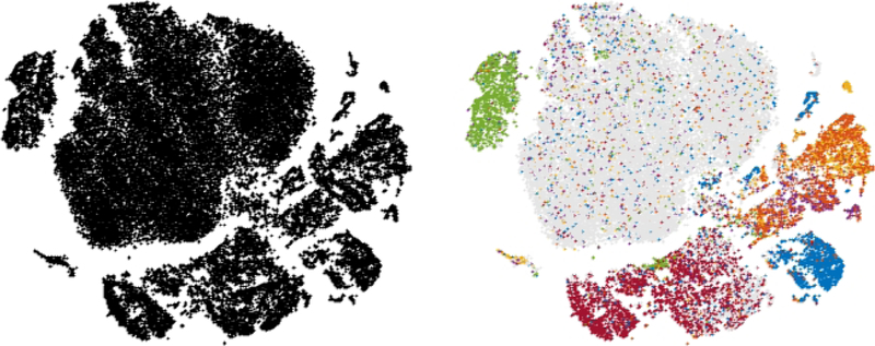
As an unsupervised learning method, t-SNE is commonly used to visualize high dimensional data and provide crucial intuition in settings where ground truth is unknown. The analysis of single cell RNA sequencing (scRNA-seq) data, where t-SNE has become an integral part of the standard analysis pipeline, provides a relevant example of its usage. Figure 1.1 shows (left) the output of running t-SNE on the 30 largest principal components of the normalized expression matrix of 49300 retinal cells taken from Macosko et al. (2015). The output on the right has cells colored based on which of 12 cell type marker genes were most expressed (with grey signifying that none of the marker genes were expressed). This example is well suited to showcase both the tremendous impact of t-SNE in the medical sciences as well as the inherent difficulties of interpreting its output when ground truth is unknown: how many clusters are in the original space, and do they correspond one-to-one to clusters in the t-SNE plot? Do the clusters (e.g. the largest cluster that does not express any marker genes) have substructure that is not apparent in this visualization? Pre-processing steps will yield different embeddings; how stable are the clusters? All these questions are of the utmost importance and underline the need for a better theoretical understanding.

Figure 1.1:

t-SNE output (left) and colored by some known ground truth (right).

1.2. Early Exaggeration.

t-SNE (described in greater detail in §3) minimizes the Kullback-Leibler divergence between a Gaussian distribution modeling distances between points in the high dimensional input space and a Student t-distribution modeling distances between corresponding points in a low dimensional embedding. Given a d-dimensional input dataset $\mathcal{X}=\left\{x_1,x_2,\dots ,x_n\right\}\subset {ℝ}^d$, t-SNE computes an s-dimensional embedding of the points in $\mathcal{X}$, denoted by $\mathcal{Y}=\left\{y_1,y_2,\dots ,y_n\right\}\subset {ℝ}^s$, where s ≪ d and most commonly s = 2 or 3. The main idea is to define a series of affinities p_ij on $\mathcal{X}$ as well as a series of affinities q_ij in the embedding $\mathcal{Y}$ and then try minimize the distance of these distributions in the Kullback-Leibler distance

$$C(\mathcal{Y})=KL(P\Vert Q)=\sum _{i\ne j}{p}_{ij}\text{log}\frac{p_{ij}}{q_{ij}},$$

which gives rise to a gradient descent method via

$$\frac{\partial C}{\partial y_i}=4\sum _{j\ne i}\left(p_{ij}-q_{ij}\right)q_{ij}Z\left(y_i-y_j\right)$$

where Z = Σ_k≠l(1 + ∥yk − yl∥²)⁻¹. One difficulty is that the speed with which the algorithm converges slows down as the number of points n increases, the algorithm requires many more iterations to converge. However, already the original paper van der Maaten and Hinton (2008) proposes a number of ways in which the convergence can be accelerated.

A less obvious way to improve the optimization, which we call ‘early exaggeration’, is to multiply all of the p_ij’s by, for example, 4, in the initial stages of the optimization. […] In all the visualizations presented in this paper and in the supporting material, we used exactly the same optimization procedure. We used the early exaggeration method with an exaggeration of 4 for the first 50 iterations (note that early exaggeration is not included in the pseudocode in Algorithm 1). (from: van der Maaten and Hinton (2008))

It is easy to test empirically that this renormalization indeed improves the clustering and is effective. It has become completely standard and is hard-coded into the very widely used standard implementation available online, as described by van der Maaten (2014):

During the first 250 learning iterations, we multiplied all p_ij–values by a userdefined constant α > 1. […] this trick enables t-SNE to find a better global structure in the early stages of the optimization by creating very tight clusters of points that can easily move around in the embedding space. In preliminary experiments, we found that this trick becomes increasingly important to obtain good embeddings when the data set size increases [Emphasis GL & SS], as it becomes harder for the optimization to find a good global structure when there are more points in the embedding because there is less space for clusters to move around. In our experiments, we fix α = 12 (by contrast, van der Maaten and Hinton (2008) used α = 4). (from: van der Maaten (2014))

As it turns out, this simple optimization trick can be rigorously analyzed. As a byproduct of our analysis, we see that the convergence of non-accelerated t-SNE will slow down as the number of points n increases and the number of iterations required will grow at least linearly in n. The implementation available online counteracts this problem by various methods: (1) the early exaggeration factor α, (2) a large (h = 200) stepsize in the gradient descent

$$y_i(t+1)=y_i(t)-h\frac{\partial C}{\partial y_i(t)},$$

and by (3) optimization techniques such as momentum. We only deal with the t-SNE algorithm, the early exaggeration factor α and the step-size h; one of the main points of our paper is that a suitable parameter selection of α and h makes it possible to guarantee fast convergence without additional optimization techniques.

1.3. Summary of Main Results.

We will now state our main results at an informal level; all the statements can be made precise (this is done in §3.2) and will be rigorously proven.

1. Canonical parameters and exponential convergence.

There is a canonical setting for the parameters α,h for which the algorithm applied to clustered data converges provably at an exponential rate without the use of other optimization techniques (such as momentum). This setting is

$$\alpha ~\frac{n}{10}\text{ and }h~1.$$

These parameters lead to an exponential convergence of all embedded clusters to small balls (whose diameter depends on how well $\mathcal{X}$ is clustered). Generally, the speed of convergence is exponential with an exponential factor κ

$$\kappa ~1-\frac{\alpha h}{n}.$$

The restriction αh ≤ n is not artificial, easy experiments show that the algorithm generally fails (no longer converges) as soon as αh ≥ 2n.

2. Spectral clustering.

The t-SNE algorithm, in this regime, behaves like a spectral clustering algorithm (defined in Section §4.1); moreover, this algorithm can be written down explicitly. This allows for (1) the use of theory from spectral clustering to rigorously analyze t-SNE and (2) a fast implementation that can perform the early exaggeration phase in a fraction of the time necessary to run t-SNE (in this regime). It also poses the challenge of trying to understand whether t-SNE behaves qualitatively different for the standard parameters α ~ 12,h ~ 200 or whether it behaves more or less identically (and thus like a spectral method).

3. Disjoint clusters.

It is not guaranteed that the embedded clusters in $\mathcal{Y}$ are disjoint; but given a random initialization, it is extremely unlikely that two distinct clusters will converge to the same center. Furthermore, if $\mathcal{X}$ is well-clustered, the diameter of the clusters $\mathcal{Y}$ can be made even smaller by decreasing the step-size h and further increasing α as long as the product satisfies αh ~ n/10. Increasing α will resolve overlapping clusters, as long as they have different centers. In particular, the number of disjoint clusters in $\mathcal{Y}$ is a lower bound on the number of clusters in $\mathcal{X}$ (and, generically, the numbers coincide). Finally, we note that since the appearance of the preprint for this manuscript, Arora et al. (2018) built upon our analytic framework to show that clusters will effectively be disjoint, under a slightly different set of assumptions.

4. Independence of initialization.

All these results are independent of the initialization of $\mathcal{Y}$ as long as it is contained in a sufficiently small ball.

An immediate implication of (3) is the following: if we are given some clustered data $\mathcal{X}$ and see that the embedding of t-SNE for large values of α (and small values of h) produces k clusters, then there are exactly k clusters in $\mathcal{X}$. The results guarantee that all clusters in $\mathcal{X}$ are eventually mapped to small balls which can be made arbitrarily small. We see that when parameters are chosen optimally, this result provides a justification for the way t-SNE is commonly used in, say, biomedical research. However, we emphasize that this result only applies to data which is well-clustered, as made precise in §3.2.

1.4. Approximating Spectral Clustering.

The fact that t-SNE approximates a spectral clustering method for α ~ n/10, h ~ 1 raises a fascinating question: does t-SNE, in its early exaggeration phase, perform better with the classical parameter choices of α ~ 12,h ~ 200 than it does with α ~ n/10, h ~ 1? If yes, then its inner workings may give rise to improved spectral methods. If no, then it would be advantageous to use α ~ n/10, h ~ 1, which then, however, is essentially a spectral method and it may be advantageous (and much faster) to initialize the second phase of t-SNE by using the outcome of a more advanced spectral method as initialization instead. We discuss some experiments in that direction in §4.1 and believe this to be worthy of further investigation. Moreover, we describe a visualization technique in the style of t-SNE for spectral clustering tools (see §4.2).

1.5. Organization.

The Organization of this paper is as follows: we first illustrate our main points with some numerical examples in Section §2. Section §3 establishes notation and a formal statement of our main result, Section §4 derives a connection between t-SNE and spectral clustering, Section §5 discusses a certain type of discrete dynamical system on finite numbers of points and establishes a crucial estimate, Section §6 gives a proof of the main result.

2. Numerical examples.

This section discusses a number of numerical examples to illustrate our main points.

2.1. Lines and Swiss roll.

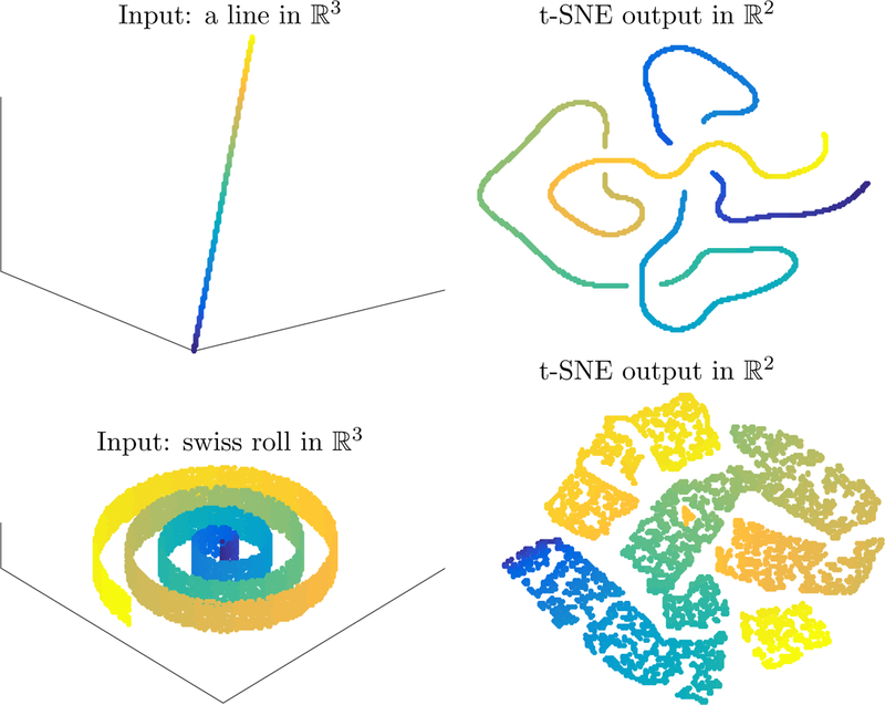
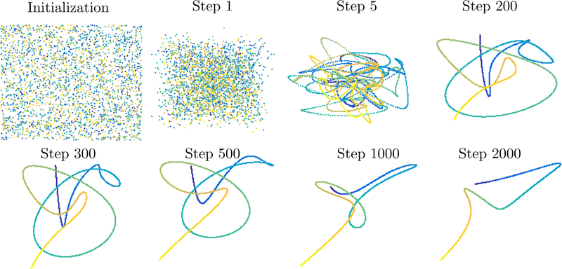
It is classical that t-SNE does not successfully embed the swiss roll; however, the random initialization causes difficulty even on simpler data: Figure 2.1 shows the t-SNE embedding (using Matlab implementation of van der Maaten (2014) with default parameters) of a simple line in ${ℝ}^3$.

Figure 2.1:

Classical t-SNE embeddings of a line and the swiss roll.

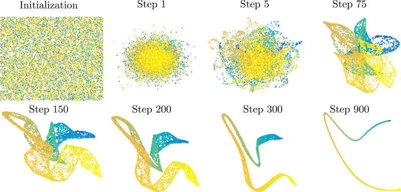
The randomized initialization causes, after initial contraction in the early exaggeration phase, a topological interlocking that cannot be further resolved. The example is even more striking with the swiss roll, where the random initialization leads to ‘knots’ that cannot be untied by t-SNE. In stark contrast, the parameter selection

$$\alpha ~\frac{n}{10}\text{ and }h~1$$

allows for a more effective early exaggeration phase that clearly recovers the line from random initial data and even contracts the swiss roll to a correctly ordered line (that would then expand in the second phase of the algorithm).

The successful embedding of these examples when α and h are chosen optimally is consistent with our claim that in this regime, the early exaggeration phase of t-SNE acts like a spectral method, many of which also correctly embed these manifolds.

2.2. Real-life data.

Finally, we show the impact of the parameter selection α ~ n/10,h ~ 1 in a real-life example. Figure 2.4 shows (left) classical out-of-the-box t-SNE on 10000 randomly subsampled handwritten digits (0–5) from the MNIST data set as well as the outcome of the early exaggeration phase of t-SNE with parameters α ~ n/10,h ~ 1 (middle) and the final outcome after the second phase of t-SNE has been initialized with the data shown in the middle (right). We see that early exaggeration does essentially all the clustering already and the second phase rearranges them. This behavior is typical: the clustering and global organization occurs in the early exaggeration phase – when the points can move most easily – and then during the rest of the iterations they often expand to fill a larger area, revealing more of the within-cluster variability that is often of interest. As evident in this figure, the second phase often improves separation between clusters, because when α = 1 the repulsive forces are no longer negligible, and the clusters hence repulse one another.

Figure 2.4:

A real-life example: classical t-SNE (left), t-SNE with our proposed parameter selection both after the early exaggeration phase (middle) and final output (right).

We believe this example again hints at one of the fundamental questions that arises from the work in this paper: is the initial clustering done by standard t-SNE comparable to the initial clustering with the new parameter selection? If so, then the fact that the new parameter selection emulates a spectral clustering method (see §4) certainly suggests the option of initializing with other clustering methods as opposed to random initialization. Moreover, it would hint at the danger of using a spectral clustering method and t-SNE as a dual verification of clustering.

3. t-SNE: Notation and the Main result.

This section starts with a complete discussion of t-distributed Stochastic Neighbor Embedding, partly for the convenience of the reader and partly to establish terminology and notation, and then describes the main result.

3.1. t-SNE.

We denote the d-dimensional input dataset by $\mathcal{X}=\left\{x_1,x_2,\dots ,x_n\right\}\subset {ℝ}^d$, t-SNE computes an s-dimensional embedding of the points in $\mathcal{X}$, denoted by $\mathcal{Y}=\left\{y_1,y_2,\dots ,y_n\right\}\subset {ℝ}^s$, where s ≪ d and most commonly s = 2 or 3. The joint probability p_ij measuring the similarity between x_i and x_j is computed as:

$$p_{i|j}=\frac{\text{exp}\left(-\Vert x_i-x_j{\Vert }^2/2{\sigma }_i^2\right)}{{\sum }_{k\ne i}\text{exp}\left(-\Vert x_i-x_k{\Vert }^2/2{\sigma }_i^2\right)}\text{ and }{p}_{ij}=\frac{p_{i|j}+p_{j|i}}{2n}.$$

The bandwidth of the Gaussian kernel, σ_i, is often chosen such that the perplexity of P_i matches a user defined value, where P_i is the conditional distribution across all data points given x_i. We will never deal with these issues: we will assume that the p_ij are given and that they correspond to a well-clustered set $\mathcal{X}$ (in a precise sense defined below). In particular, we will not assume that they have been obtained using a Gaussian kernel. The similarity between points y_i and y_j in the low dimensional embedding is defined as:

$$q_{ij}=\frac{{\left(1+\Vert y_i-y_j{\Vert }^2\right)}^{-1}}{{\sum }_{k\ne l}{\left(1+\Vert y_k-y_l{\Vert }^2\right)}^{-1}}.$$

t-SNE finds the points {y₁,…,y_n} which minimize the Kullback-Leibler divergence between the joint distribution P of points in the input space and the joint distribution Q of points in the embedding space:

$$C(\mathcal{Y})=KL(P\Vert Q)=\sum _{i\ne j}{p}_{ij}\text{log}\frac{p_{ij}}{q_{ij}}.$$

The points $\mathcal{Y}$ are initialized randomly, and the cost function $C\left(\mathcal{Y}\right)$ is minimized using gradient descent. The gradient is derived in Appendix A of van der Maaten and Hinton (2008):

$$\frac{\partial C}{\partial y_i}=4\sum _{j\ne i}\left(p_{ij}-q_{ij}\right)q_{ij}Z\left(y_i-y_j\right)$$

where Z is a global normalization constant

$$Z=\sum _{k\ne l}{\left(1+\Vert y_k-y_l{\Vert }^2\right)}^{-1}.$$

As in van der Maaten (2014), we split the gradient into two parts:

$$\frac{1}{4}\frac{\partial C}{\partial y_i}=\sum _{j\ne i}{p}_{ij}{q}_{ij}Z\left(y_i-y_j\right)-\sum _{j\ne i}{q}_{ij}^{2}Z\left(y_i-y_j\right).$$

Since we are interested in the minimization of the functional, we would naturally step in direction of the negative gradient

$$-\frac{1}{4}\frac{\partial C}{\partial y_i}=\sum _{j\ne i}{p}_{ij}{q}_{ij}Z\left(y_j-y_i\right)-\sum _{j\ne i}{q}_{ij}^{2}Z\left(y_j-y_i\right).$$

Each of these two terms has a very natural interpretation, the first term is usually called the attractive term while the second term describes a repulsive force (see, for example, van der Maaten and Hinton (2008) for use of this terminology). The reason is simple: the first term is moving y_i to a weighted average of the other y_j. The weights are big if the underlying points are close in space and small if they are far away. The second term has the opposite sign and thus exerts the opposite effect, however, the degree of repulsion depends solely on the closeness of points in the embedding space. Put differently, the first term attracts terms that are meant to be together based on distance in the original space and the second term tries to push points apart when they get too close in the embedding space regardless of whether they are meant to be close to each other or not. One would hope that attractive forces win out over the repulsion for points that are meant to be close to each other and loses out for points that are meant to be far apart from each other and this is one of the common interpretations of the underlying mechanism. Early exaggeration introduces the coefficient α > 1 and corresponds to the gradient descent method

$$\frac{1}{4}\frac{\partial C}{\partial y_i}=\sum _{j\ne i}\alpha p_{ij}{q}_{ij}Z\left(y_i-y_j\right)-\sum _{j\ne i}{q}_{ij}^{2}Z\left(y_i-y_j\right)$$

and a small step-size h > 0 leads to the expression

$$\frac{h}{4}\frac{\partial C}{\partial y_i}=h\sum _{j\ne i}\alpha p_{ij}{q}_{ij}Z\left(y_i-y_j\right)-h\sum _{j\ne i}{q}_{ij}^{2}Z\left(y_i-y_j\right).$$

3.2. Main result.

This section gives our main result. We emphasize that the method of proof is rather flexible and it is not difficult to obtain variations on the result under slightly different assumptions. We emphasize that our result is formally stated for a set of points {x₁,…,x_n} and a set of mutual affinities p_ij. We will not assume that the p_ij are obtained using the standard t-SNE normalizations but work at a full level of generality using a set of three assumptions. We note, and explain below, that for standard t-SNE the second assumption holds until the number of points exceeds, roughly, n ~ 20000 and the third assumption holds by design. The first assumption encapsulates our notion of clustered data.

1. $\mathcal{X}$ is clustered.

We proceed by giving a very versatile definition of what it means to be a cluster; it is also applicable to things that clearly are not clusters, however, in those cases the error bound in the Theorem will not convey any information. Formally, we assume that there exists a $k\in \mathbb{N}$ (the number of clusters) and a map π: {1,…,n} → {1,2,…,k} assigning each point to one of the k clusters such that the following property holds: if π(x_i) = π(x_j), then

$$p_{ij}\ge \frac{1}{10n\left|{\pi }^{-1}(\pi (i))\right|}.$$

The constant 10 is fairly arbitrary in the sense that any absolute constant will do (but slow down the speed of convergence as it gets larger); we put 10 to avoid an overly complicated exposition. Observe that |π⁻¹(π(i))| is merely the size of the cluster in which i and j lie. We will furthermore abbreviate, for fixed 1 ≤ i ≤ n, summations over clusters as

$$\underset{\text{same cluster}}{\sum _{j\ne i}}:=\underset{\pi (j)=\pi (i)}{\sum _{j\ne i}}\text{and}\underset{\text{other clusters}}{\sum _{j\ne i}}:=\underset{\pi (j)=\pi (i)}{\sum _{j\ne i}}$$

The condition on p_ij above implies that

$$\underset{\text{same cluster}}{\sum _{j\ne i}}{p}_{ij}\ge \frac{1}{10n}\text{ for all }1\le i\le n.$$

This assumption ensures that elements are at least somewhat connected within their cluster; that is, we lower bound the affinity of each point to the other points in its cluster. We emphasize that it is a rather weak assumption since we do not simultaneously demand that the sum over all other elements is small. Indeed, one of the leading-error terms in the Theorem is

$$\text{ the quantity }\underset{\text{other clusters}}{\sum _{j\ne i}}{p}_{ij},$$

so if the data is strongly clustered and the p_ij have been obtained in one of the usual ways, then the optimal choice of π will be exactly the one that minimizes this quantity uniformly over all i and will then correspond to the original clustering; however, any other map π: {1,…,n} → {1,2,…,k} is equally admissible but is likely to result in a large (trivial, uninformative) error bound. In particular, our assumptions on what it means to be clustered are so weak that a given data set does not necessarily have a unique decomposition into different clusters, and this is mirrored in the main result that does not imply cluster separation (we refer to Arora et al. (2018) for such a statement under different assumptions).

2. Parameter choice.

Our second assumption ensures that the step size in the gradient descent, a quantity determined by the step size h and the exaggeration parameter α as the product αh, is within a reasonable regime. An assumption along these lines is clearly necessary for general gradient descent techniques to avoid overoscillation (i.e. missing a local minima and moving too far in the other direction). More precisely, we assume that α and h are chosen such that, for some 1 ≤ i ≤ n

$$\frac{1}{100}\le \alpha h\underset{\text{same cluster}}{\sum _{j\ne i}}{p}_{ij}\le \frac{9}{10}.$$

The main result will be applicable to single cluster (i.e. it is possible to guarantee that a single cluster converges even if the rest does not) and it can be applied to exactly those clusters satisfying this inequality. It is easy to see, both in the proof and in numerical experiments, that the upper bound is a necessary condition for the early exaggeration phase of t-SNE to work (more precisely, the upper bound 1 is necessary but we need a little bit of leeway in another part of the argument). We observe that condition (1) implies that α ~ n/10 and h ~ 1 is admissible, however, other parameter choices (i.e. α ~ 10n, h ~ 1/100) are equally valid. As the number of points gets larger, the lower bound is violated: our main result can be easily extended to cover that case, however, the factor κ with which exponential convergence occurs approaches 1 and convergence, while technically exponential, becomes slow. In particular, an analysis of how this condition acts in the proof motivates an accurate parameter selection rule.

Guideline.

The best convergence rate for the cluster containing y_i is attained when

$$\alpha h=\frac{9}{10}{\left(\underset{\text{same cluster}}{\sum _{j\ne i}}{p}_{ij}\right)}^{-1}\text{ while }\alpha h=\frac{9}{10}{\left(\underset{1\le i\le n}{\text{max}}\underset{\text{same cluster}}{\sum _{j\ne i}}{p}_{ij}\right)}^{-1}$$

is the best selection to ensure that all clusters converge.

We also observe that in the setting where the parameters are not chosen optimally (e.g. convergence rate κ ~ 1), momentum can be useful to accelerate convergence. However, for t-SNE there are currently no rigorous results in that direction.

3. Localized initialization.

The initialization satisfies $\mathcal{Y}\subset {[-0.01,0.01]}^2$. This assumption is not crucial and could be easily modified at the cost of changing some other constants. The proof suggests that initializing at smaller scales might be beneficial on the level of constants.

We can now state our main result.

Theorem 3.1 (Main Result).

Under Assumptions (1)–(3), the diameter of the embedded cluster {y_j: 1 ≤ j ≤ n ∧ π(j) = π(i)} decays exponentially (at universal rate) until its diameter satisfies, for some universal c > 0,

$$\text{diam}\left\{y_j:1\le j\le n\wedge \pi (j)=\pi (i)\right\}\le c\cdot h\left(\alpha \underset{otherclusters}{\sum _{j\ne i}}{p}_{ij}+\frac{1}{n}\right).$$

Remarks.

1. The Theorem can be applied to a single cluster; in particular, some clusters may contract to tiny balls while others do not contract at all.

2. Since αh ~ n, we see that the bound is only nontrivial if, for some small constant c₂ > 0,

   $$\underset{\text{other clusters }}{\sum _{j\ne i}}{p}_{ij}\le \frac{c_2}{n}.$$

   Otherwise, it merely tells us that the elements of the clusters are contained in a ball of radius ~ 1 (as are all the other points): this is not an artifact of the proof, but clearly necessary. If the affinity to other clusters is large, the data is not well-clustered. Generally, for well-clustered data, we would expect that sum to be very close to 0 which would yield a leading term error of ch/n.

3. The constant c seems to be roughly on scale c ~ 10 for well-clustered data and slightly larger for data with worse clustering properties (in particular, for the classical t-SNE parameter section, it would slowly increase with the number of points n). We believe this estimate to be too conservative and consider the true value to be on a smaller order of magnitude; this question will be pursued in future work.

The proof of the main result is actually rather versatile and should easily adapt to a variety of other settings that might be of interest. This versatility is partly due to the connection of the argument to rather fundamental ideas in partial differential equations, indeed, the argument may be interpreted as a maximum principle for a discrete parabolic operator acting on vector-valued (i.e. points in space) data. This interpretation is what led us to establish a connection to spectral clustering which we now discuss.

4. A Connection to Spectral Clustering.

The purpose of this section is to note a connection to spectral clustering (Laplacian eigenmaps, see Belkin and Niyogi (2003)); the fact that the main terms coincide has previously been noted by Carreira-Perpinan (2010).

4.1. Approximating spectral clustering.

We give a quantitative description: it is possible to take the limit α → ∞, h → 0 (scaled so that α · h = const) and that, in that limit, one obtains a simple spectral clustering method. We re-introduce notation and assume again that $\mathcal{X}=\left\{x_1,x_2,\dots ,x_n\right\}\subset {ℝ}^d$ is given. We assume p_ij is some collection of affinities scaled in such a way that for x_i,x_j in the same cluster π(i) = π(j)

$$p_{ij}\ge \frac{1}{10}\frac{1}{\left|{\pi }^{-1}(\pi (i))\right|}\text{ and }\sum _{j=1}^n{p}_{ij}\le 1.$$

We observe that this scaling is slightly differently than the one above: it is obtained by absorbing the αh ~ n term into the affinities. At the same time, h → 0 implies that the repulsion term containing the q_ij does not exert any force. This implies that, in the limit, the remaining term in the gradient descent method is given by

$$\begin{gathered} y_i(t+1)=y_i(t)+\sum _{j\ne i}{p}_{ij}\left(y_j(t)-y_i(t)\right) \\ =\sum _{j\ne i}{p}_{ij}{y}_j(t)+\left(1-\sum _{j\ne i}{p}_{ij}\right)y_i(t). \end{gathered}$$

This, however, can be interpreted as a Markov chain with suitably chosen transition probabilities. It may be unusual, at first, to see this equation since the y_i(t) are vectors in ${ℝ}^2$, however, all the equations separate different coordinates, which allows for a reduction to the familiar form. All the canonical results from spectral clustering apply: the asymptotic behavior is given by the largest non-trivial eigenvalue(s), which are either 1 (in the case of perfectly separated clusters) or very close to 1 and convergence speed depends on the spectral gap. Note, in particular, that for generic data the largest eigenvector is constant; however, since the algorithm is only run for a small number of steps, we essentially recover the dominant eigenvectors and the second phase of t-SNE then re-expands the clusters.

4.2. Visualizing spectral clustering.

The connection also allows us to go the other direction and discuss a particular visualization technique for spectral methods that shows arising clusters as points in ${ℝ}^2$ (or higher dimensions, which is not essential here). The transition matrix of the Markov chain is given by

$$A_{ij}=\{\begin{array}{ll}1-\sum _{i\ne k}{p}_{ik}\hfill & \text{if }i=j\hfill \\ p_{ji}\hfill & \text{otherwise.}\hfill \end{array}$$

The large-time behavior of y(t) = A^ty(0) is essentially determined by the spectrum of A close to 1. Moreover, in the case of perfect clustering with p_ij = 0 whenever x_i and x_j are in different clusters, there are exactly k eigenvalues equal to 1 and the initialization converges to that. Let us now assume that the goal is visualization in ${ℝ}^2$. We let $\mathcal{Y}=\left\{y_1(0),y_2(0),\dots ,y_n(0)\right\}\subset {ℝ}^2$ be a set of points that we assume are i.i.d. random variables from, say, the uniform distribution on [−0.01,0.01]². We propose to visualize the point set after k iterations as follows: collect these n initial vectors in a n × 2 vector y and interpret the n rows of A^ky as coordinates in ${ℝ}^2$. This creates t-SNE-style visualizations for spectral methods (see Fig. 4.1 and Fig. 4.2, lower rows).

Figure 4.1:

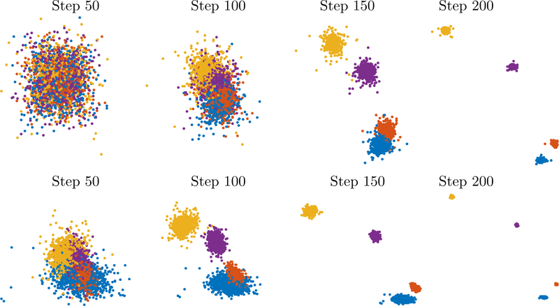
Early exaggeration via t-SNE with α = n/10, h = 1 (top) and visualization of iterations of the spectral method (bottom) on same initialization.

Figure 4.2:

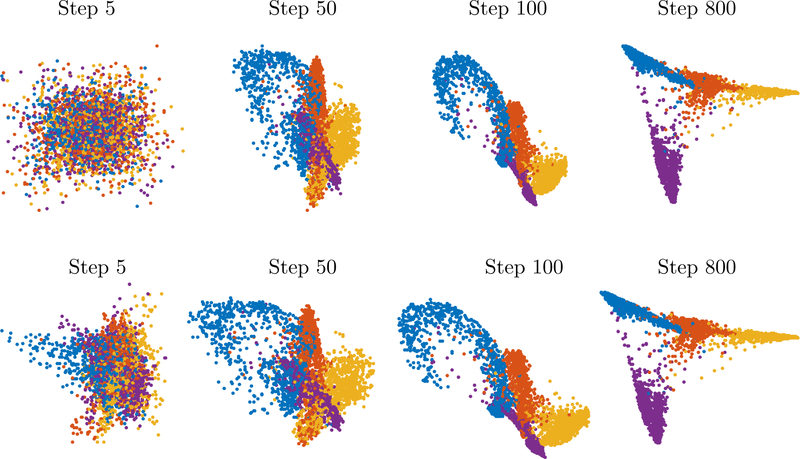
Early exaggeration via t-SNE with α ~ n/3, h = 1 (top, parameter selection via guideline) and iterations of the spectral method (bottom).

Examples.

An example of this method is shown in Figure 4.1. The example is comprised of 40000 points in ${ℝ}^{25}$ sampled from four very narrow Gaussians and are highly clustered. We used perplexity of 30 to create the p_ij and used α = n/10,h = 1 in the implementation of t-SNE. The second row in Figure 4.1 shows the projection onto the 50 largest eigenvectors of A. The computation time of t-SNE took roughly 7 minutes vs. 1 minute for the spectral decomposition – note, however, that once the spectral decomposition has been computed, then iterations can be computed in constant time (one only has to raise the eigenvalues to some power). Another example is given in Figure 4.2 that is run on 4 digits in MNIST; again, both methods coincide. This demonstrates that our derivation of the approximating spectral method was accurate. At the same time, it suggests to repeat the fundamental question.

Open problem.

Is the clustering behavior of the early exaggeration phase of t-SNE with α = 12, h = 200 (and possibly optimization techniques such as momentum) essentially qualitatively equivalent to the behavior of t-SNE with our parameter choice α = n/10,h = 1?

If this were indeed the case, then the early exaggeration phase of t-SNE would be simply a spectral clustering method in disguise; if not, then it would be very valuable to understand under which circumstances its performance is superior to spectral clustering and whether its underlying mechanisms could be used to boost spectral methods. We reiterate that we believe this to be a very interesting problem.

5. Ingredients for the Proof: Discretized Dynamical Systems.

This section introduces a type of discrete dynamical systems on sets of points in ${ℝ}^s$ and we describe their asymptotic behavior; this is a self-contained result; it could potentially be interpreted as an analysis of a spectral method that is robust to small error terms but the analysis is simple enough for us to keep entirely self-contained. Our original guiding picture was that of the maximum principle in the theory of parabolic partial differential equations.

5.1. A discrete dynamical system.

Let $z_1,\dots ,z_n\in {ℝ}^s$ be given. We use them as initial values for a time-discrete dynamical system that is defined via

$$\begin{gathered} z_i(t+1)=z_i(t)+\sum _{j=1}^n{\alpha }_{i,j,t}\left(z_j(t)-z_i(t)\right)+{\epsilon }_i(t) \\ {z}_i\left(0\right)=z_i \end{gathered}$$

At this stage, if the points are in general position and n ≥ s, basic linear algebra implies that this system can undergo almost any arbitrary evolution as long as one is free to choose α_i,j,t.

We will henceforth assume that these parameters assume the following three conditions.

1. There is a uniform lower bound on the coefficients for all t > 0 and all i ≠ j

   $$\left|{\alpha }_{i,j,t}\right|\ge \delta >0.$$
2. There is a uniform upper bound on the coefficients

   $$\sum _{j=1}^n{\alpha }_{i,j,t}\le 1.$$
3. There is a uniform upper bound on the error term

   $$\Vert {\epsilon }_i(t)\Vert \le \epsilon .$$

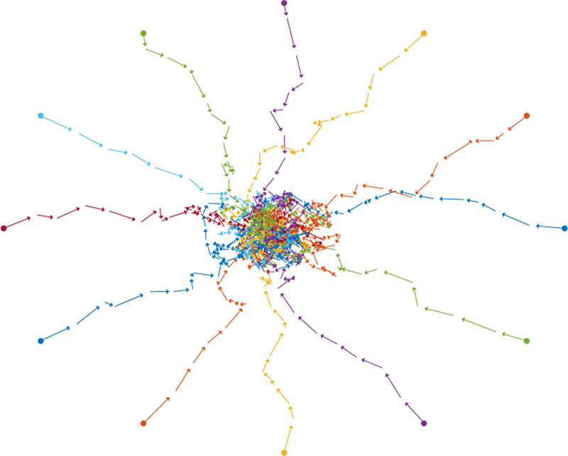
A typical example of such a dynamical system is given in the Figure below: we start with twelve points on the unit circle and then iterate the system for some random choices of a_i,j,t and random ε_i(t). The points move at first towards each other until they are close and the error term starts being on the same scale as the forces of attraction. The points then move around randomly (all the while staying close to each other). We will make this intuitive picture precise below. The main result of this section is that all the points in this dynamical system are eventually contained in a ball whose size only depends on n, δ and ε. We start by showing that the convex hull of the points is stable. We use B(0, ε) to denote a ball of radius ε, A + B = {a + b: a ∈ A ∧ b ∈ B} and conv A for the convex hull of A.

Lemma 5.1 (Stability of the convex hull).

With the assumptions above, we have

$$\text{conv}\left\{z_1(t+1),z_2(t+1),\dots ,z_n(t+1)\right\}\subseteq \text{conv}\left\{z_1(t),z_2(t),\dots ,z_n(t)\right\}+B(0,\epsilon ),$$

Proof.

This argument is simple. We note that

$$\begin{gathered} z_i(t+1)=z_i(t)+\sum _{j=1}^n{\alpha }_{i,j,t}\left(z_j(t)-z_i(t)\right)+{\epsilon }_i(t) \\ =\left(1-\underset{j\ne i}{\sum _{j=1}^n}{\alpha }_{i,j,t}\right)z_i(t)+\underset{j\ne i}{\sum _{j=1}^n}{\alpha }_{i,j,t}{z}_j(t)+{\epsilon }_i(t). \end{gathered}$$

By assumption,

$$0\le \sum _{j=1}^n{\alpha }_{i,j,t}\le 1$$

and this implies z_i(t + 1) − ε_i(t) ∈ conv{z₁(t),z₂(t),…,z_n(t)}. ∎

Lemma 5.2 (Contraction inequality).

With the notation above, if the diameter is large

$$\text{diam}\left\{z_1(t),z_2(t),\dots ,z_n(t)\right\}\ge \frac{10\epsilon }{n\delta },$$

then

$$\text{diam}\left\{z_1(t+1),z_2(t+1),\dots ,z_n(t+1)\right\}\le \left(1-\frac{n\delta }{20}\right)\text{diam}\left\{z_1(t),z_2(t),\dots ,z_n(t)\right\}.$$

One particularly important consequence is the following: the diameter shrinks, at an exponential rate (1 − nδ/20)^t, to a size of ~ ε/(nδ). Of course, this convergence is particularly fast whenever nδ ~ 1. It is easy to see, for example by taking n = 2 points in $ℝ$, that this is the optimal scale for the result to hold.

Proof.

The method of proof will be as follows: we will project the set of points onto an arbitrary line (say, the x−axis by taking only the first coordinate of each point) and show that the one-dimensional projections contract exponentially quickly. This then implies the desired statement. Let ${\pi }_x:{ℝ}^n\to ℝ$ be such a projection. We abbreviate the diameter of the projection as

$$\text{diam}:=\text{diam}\left\{{\pi }_x{z}_1(t),{\pi }_x{z}_2(t),\dots ,{\pi }_x{z}_n(t)\right\}.$$

We may assume w.l.o.g. that this set is contained in {π_xz₁(t),π_xz₂(t),…,π_xz_n(t)} ⊂ [0,diam]. We then subdivide the interval into two regions

$$I_1=\left[0,\frac{\text{diam}}{2}\right]\text{ and }{I}_2=\left(\frac{\text{diam}}{2},\text{diam}\right]$$

and denote the number of points in each interval by i₁,i₂. Clearly, i₁ + i₂ = n and therefore either i₁ ≥ n/2 or i₂ ≥ n/2. We assume w.l.o.g. the first case holds. Projections are linear, thus

$${\pi }_x{z}_i(t+1)={\pi }_x{z}_i(t)+\sum _{j=1}^n{a}_{i,j,t}{\pi }_x\left(z_j(t)-z_i(t)\right)+{\pi }_x{\epsilon }_i(t).$$

We abbreviate

$$0\le \sigma :=\sum _{j=1}^n{\alpha }_{i,j,t}\le 1$$

and write

$$\begin{gathered} \sum _{j=1}^n{a}_{i,j,t}{\pi }_x\left(z_j(t)-z_i(t)\right)=\sum _{{\pi }_x{z}_j\le \text{diam}/2}^n{a}_{i,j,t}{\pi }_x\left(z_j(t)-z_i(t)\right)+\sum _{{\pi }_x{z}_j>\text{diam}/2}^n{a}_{i,j,t}{\pi }_x\left(z_j(t)-z_i(t)\right) \\ \le \sum _{{\pi }_x{z}_j\le \text{diam}/2}^n{a}_{i,j,t}\left(\frac{\text{diam}}{2}-{\pi }_x{z}_i(t)\right)+\sum _{{\pi }_x{z}_j>\text{diam}/2}^n{a}_{i,j,t}\left(\text{diam}-{\pi }_x{z}_i(t)\right) \\ =\sum _{{\pi }_x{z}_j\le \text{diam}/2}^n{a}_{i,j,t}\frac{\text{diam}}{2}+\sum _{{\pi }_x{z}_j>\text{diam}/2}^n{a}_{i,j,t}\text{diam}-\sigma {\pi }_x{z}_i(t). \end{gathered}$$

■

Moreover, using the lower bound a_i,j,t ≥ δ

$$\begin{gathered} \text{diam}\left(\frac{1}{2}\sum _{{\pi }_x{z}_j\le \text{diam}/2}^n{a}_{i,j,t}+\sum _{{\pi }_x{z}_j>\text{diam}/2}^n{a}_{i,j,t}\right)\le \text{diam}\left(\sigma -\frac{1}{2}\sum _{{\pi }_x{z}_j\le \text{diam}/2}^n{a}_{i,j,t}\right) \\ \le \left(\sigma -\frac{n\delta }{4}\right)\text{ diam.} \end{gathered}$$

Then, however,

$$\begin{gathered} {\pi }_x{z}_i(t+1)={\pi }_x{z}_i(t)+\sum _{j=1}^n{a}_{i,j,t}{\pi }_x\left(z_j(t)-z_i(t)\right)+{\pi }_x{\epsilon }_i(t) \\ \le (1-\sigma ){\pi }_x{z}_i(t)+\left(\sigma -\frac{n\delta }{4}\right)\text{diam}+{\pi }_x{\epsilon }_i(t) \\ \le (1-\sigma )\text{diam}+\left(\sigma -\frac{n\delta }{4}\right)\text{diam}+{\pi }_x{\epsilon }_i(t) \\ =\left(1-\frac{n\delta }{4}\right)\text{diam}+{\pi }_x{\epsilon }_i(t) \end{gathered}$$

which shows that π_xz_i(t + 1) ∈ [−ε, diam(1 − nδ/4) + ε]. This implies

$$\text{diam}\left\{{\pi }_x{z}_1(t+1),{\pi }_x{z}_2(t+1),\dots ,{\pi }_x{z}_n(t+1)\right\}\le \left(1-\frac{n\delta }{4}\right)\text{diam}+2\epsilon .$$

If the diameter is indeed disproportionately large

$$\text{diam}\ge \frac{10\epsilon }{n\delta },$$

then this can be rearranged as

$$\epsilon \le \frac{n\delta }{10}\text{ diam}$$

and therefore

$$\left(1-\frac{n\delta }{4}\right)\text{diam}+2\epsilon \le \left(1-\frac{n\delta }{4}\right)\text{diam}+\frac{n\delta }{5}\text{diam}\le \left(1-\frac{n\delta }{20}\right)\text{diam}.$$

Since this is true in every projection, it also holds for the diameter of the original set. ∎

Remark.

The argument could be slightly improved because in its current form it assumes that the error ε_i has ∥ε_i(t)∥_ℓ∞ = ε, while we assume $\Vert {\epsilon }_i(t){\Vert }_{{\mathcal{l}}^{\infty }}\le \Vert {\epsilon }_i(t){\Vert }_{{\mathcal{l}}^2}=\epsilon$. This, together with the usual other optimization schemes, should yield an improved estimate on the constant. The condition on δ could also be weakened (at the cost of losing constants). In particular, it would be sufficient in Assumption (1) in our main result to assume that, for every 1 ≤ i ≤ n

$$p_{ij}\ge \frac{1}{10n\left|{\pi }^{-1}(\pi (i))\right|}\text{ holds for at least }\left(\frac{1}{2}+\epsilon \right)\left|{\pi }^{-1}(\pi (i))\right|\text{ values of }j$$

that are in the same cluster π(z_i) = π(z_j). By adapting the proof, the constant (1/2 + ε) could be reduced further, however, this is inevitably going to decrease the provable bounds on the exponential decay rate (which is not an artifact of the method, the speed of convergence of the algorithm slows down in this setting).

6. Proof of the Main Result.

The rough outline of the argument is as follows: we initialize all points inside [−0.01,0.01]². We rewrite the gradient descent method acting on one particular embedded cluster as a dynamical system of the type studied above with an error term. The error term contains q_ij, which depend on distances between points from different clusters. This is difficult to control, especially if the points are far apart. Our strategy will now be as follows: we show that the q_ij are all under control as long as everything is contained in [−0.02,0.02]². We use stability of the convex hull to guarantee that all of the embedded points are within [−0.02,0.02]² for at least ℓ iterations and show that this time-scale is enough to guarantee contraction of the cluster.

Proof.

We start by showing that the q_ij are comparable as long as the point set is contained in a small region space. Let now {y₁,y₂,…,y_n} ⊂ [−0.02,0.02]² and recall the definitions

$$q_{ij}=\frac{{\left(1+\Vert y_i-y_j{\Vert }^2\right)}^{-1}}{\sum _{k\ne l}{\left(1+\Vert y_k-y_l{\Vert }^2\right)}^{-1}}\text{ and }Z=\sum _{k\ne l}{\left(1+\Vert y_k-y_l{\Vert }^2\right)}^{-1}.$$

Then, however, it is easy to see that 0 ≤ ∥y_i − y_j∥ ≤ 0.06 implies

$$\frac{9}{10}\le q_{ij}Z={\left(1+\Vert y_i-y_j{\Vert }^2\right)}^{-1}\le 1.$$

We will now restrict ourselves to a small embedded cluster {y_i: π(i) fixed} and rewrite the gradient descent method as

$$\begin{gathered} y_i(t+1)=y_i(t)+\underset{\text{same cluster}}{\sum _{j\ne i}}(\alpha h)p_{ij}{q}_{ij}Z\left(y_j(t)-y_i(t)\right) \\ +\underset{\text{other clusters}}{\sum _{j\ne i}}(\alpha h)p_{ij}{q}_{ij}Z\left(y_j(t)-y_i(t)\right) \\ -h\sum _{j\ne i}{q}_{ij}^{2}Z\left(y_j(t)-y_i(t)\right), \end{gathered}$$

where the first sum is yielding the main contribution and the other two sums are treated as a small error. Applying our results for dynamical systems of this type requires us to verify the conditions. We start by showing the conditions on the coefficients to be valid. Clearly,

$$\alpha h{p}_{ij}{q}_{ij}Z\ge \alpha h{p}_{ij}\frac{9}{10}\ge \frac{\alpha h}{10n\left|{\pi }^{-1}(\pi (i))\right|}\frac{9}{10}\ge \frac{9}{100}\frac{\alpha h}{\left|{\pi }^{-1}(\pi (i))\right|}~\delta ,$$

which is clearly admissible whenever αh ~ n. As for the upper bound, it is easy to see that

$$\underset{\text{ same cluster }}{\sum _{j\ne i}}(\alpha h)p_{ij}{q}_{ij}Z\le \alpha h\underset{\text{ same cluster }}{\sum _{j\ne i}}{p}_{ij}\le 1.$$

It remains to study the size of the error term for which we use the triangle inequality

$$\begin{gathered} \Vert \underset{\text{ other clusters }}{\sum _{j\ne i}}(\alpha h)p_{ij}{q}_{ij}Z\left(y_j(t)-y_i(t)\right)\Vert \le \alpha h\underset{\text{ other clusters }}{\sum _{j\ne i}}{p}_{ij}\Vert y_j(t)-y_i(t)\Vert \\ \le 0.06\alpha h\underset{\text{ other clusters }}{\sum _{j\ne i}}{p}_{ij} \end{gathered}$$

and, similarly for the second term,

$$\Vert h\sum _{j\ne i}{q}_{ij}^{2}Z\left(y_j(t)-y_i(t)\right)\Vert \le h\sum _{j\ne i}{q}_{ij}\Vert \left(y_j(t)-y_i(t)\right)\Vert \le 0.06h\sum _{j\ne i}{q}_{ij}\le \frac{0.1h}{n}.$$

■

This tells us that the norm of the error term is bounded by

$$\Vert \epsilon \Vert \le 0.1h\left(\alpha \underset{\text{ other clusters }}{\sum _{j\ne i}}{p}_{ij}+\frac{1}{n}\right).$$

It remains to check whether time-scales fit. The number of iterations ℓ for which the assumption $\mathcal{Y}\subset {[-0.02,0.02]}^2$ is reasonable is at least ℓ ≥ 0.01/ε. At the same time, the contraction inequality implies that in that time the cluster shrinks to size

$$\text{max}\left\{\frac{10\epsilon }{\left|{\pi }^{-1}(\pi (i))\right|\delta },0.01{\left(1-\frac{1}{20}\right)}^{\mathcal{l}}\right\}\le \text{max}\left\{\frac{10\epsilon }{\left|{\pi }^{-1}(\pi (i))\right|\delta },8\epsilon \right\},$$

where the last inequality follows from the elementary inequality

$${\left(1-\frac{1}{20}\right)}^{1/100\epsilon }\le 8\epsilon .$$

Remarks.

The proof is relatively flexible in several different spots. By demanding that the initialization $\mathcal{Y}$ is contained in a sufficiently small ball, one can force the quantity Zq_ij to be arbitrarily close to 1. We also emphasize that we did not optimize over constants and additional fine-tuning in various spots would yield better constants (at the cost of a more involved argument which is why we decided against it). The use of the triangle inequality in bounding the error terms is another part of the proof that deserves attention: if the clusters are spread out, then we would expect the repulsive forces to act from all directions and lead to additional cancellation (which, if it were indeed the case that the q_ij do not play a significant role in the clustering that occurs in the early exaggeration phase, would be an additional reason for the strong similarity to the outcome of the spectral method). It could be of interest to study mean-field-type approximations to gain a better understanding of this phenomenon.

Figure 2.2:

Early exaggeration phase of t-SNE on a line with α = 20n, h = 0.05.

Figure 2.3:

Early exaggeration phase of t-SNE on a swiss roll with α = n, h = 1.

Figure 5.1:

A typical evolution a dynamical system of this type.