Abstract
We use a dynamic panel data model to generate density forecasts for daily active Covid-19 infections for a panel of countries/regions. Our specification that assumes the growth rate of active infections can be represented by autoregressive fluctuations around a downward sloping deterministic trend function with a break. Our fully Bayesian approach allows us to flexibly estimate the cross-sectional distribution of slopes and then implicitly use this distribution as prior to construct Bayes forecasts for the individual time series. We find some evidence that information from locations with an early outbreak can sharpen forecast accuracy for late locations. There is generally a lot of uncertainty about the evolution of active infection, due to parameter and shock uncertainty, in particular before and around the peak of the infection path. Over a one-week horizon, the empirical coverage frequency of our interval forecasts is close to the nominal credible level. Weekly forecasts from our model are published at https://laurayuliu.com/covid19-panel-forecast/.
Keywords: Bayesian inference, Covid-19, Density forecasts, Interval forecasts, Panel data models, Random effects, SIR model
1. Introduction
This paper contributes to the rapidly growing literature on generating forecasts related to the current Covid-19 pandemic. We are adapting forecasting techniques for panel data that we have recently developed for economic applications such as the prediction of bank profits, charge-off rates, and the growth (in terms of employment) of young firms; see Liu (2020), and Liu et al., 2020, Liu et al., 2019. We focus on the prediction of the smoothed daily number of active Covid-19 infections for a cross-section of approximately one hundred countries/regions, henceforth locations. The data are obtained from the Center for Systems Science and Engineering (CSSE) at Johns Hopkins University. While we are currently focusing on country-level aggregates, our model could be easily modified to accommodate, say, state- or county-level data.
In economics, researchers distinguish, broadly speaking, between reduced-form and structural models. A reduced-form model summarizes spatial and temporal correlation structures among economic variables and can be used for predictive purposes assuming that the behavior of economic agents and policy makers over the prediction period is similar to the behavior during the estimation period. A structural model, on the other hand, attempts to identify causal relationships or parameters that characterize policy-invariant preferences of economic agents and production technologies. Structural economic models can be used to assess the effects of counterfactual policies during the estimation period or over the out-of-sample forecasting horizon.
The panel data model developed in this paper to generate forecasts of Covid-19 infections is a reduced-form model. It processes cross-sectional and time-series information about past infection levels and maps them into predictions of future infections. While the model specification is motivated by the time-path of infections generated by the workhorse compartmental model in the epidemiology literature, the so-called susceptible-infected-recovered (SIR) model, it is not designed to answer quantitative policy questions, e.g., about the impact of social-distancing measures on the path of future infection rates.
Building on a long tradition of econometric modeling dating back to Haavelmo (1944), our model is probabilistic. The growth rates of the infections are decomposed into a deterministic component which approximates the path predicted by a deterministic SIR model and a stochastic component that could be interpreted as either time-variation in the coefficients of an epidemiological model or deviations from such a model. We report interval and density forecasts of future infections that reflect two types of uncertainty: uncertainty about model parameters and uncertainty about future shocks. We model the growth rate of active infections as autoregressive fluctuations around a deterministic trend function that is piecewise linear. The coefficients of this deterministic trend function are allowed to be heterogeneous across locations. The goal is not curve fitting – our model is distinctly less flexible in samples than some other models – but rather out-of-sample forecasts, which is why we prefer to project growth rates based on autoregressive fluctuations around a parsimonious linear time trend with a single break.
A key feature of the Covid-19 pandemic is that the outbreaks did not take place simultaneously in all locations. Thus, we can potentially learn from the speed of the spread of the disease and subsequent containment in country A, to make forecasts of what is likely to happen in country B, while simultaneously allowing for some heterogeneity across locations. In a panel data setting, one captures cross-sectional heterogeneity in the data with unit-specific parameters. The more precisely these heterogeneous coefficients are estimated, the more accurate are the forecasts. A natural way of disciplining the model is to assume that the heterogeneous coefficients are “drawn” from a common probability distribution. If this distribution has a large variance, then there is a lot of country-level heterogeneity in the evolution of Covid-19 infections. If instead, the distribution has a small variance, then the path of infections will be very similar across samples, and we can learn a lot from, say, China, that is relevant for predicting the path of the disease in South Korea or Germany.
Formally, the cross-sectional distribution of coefficients can be used as a so-called a priori distribution (prior) when making inference about country-specific coefficients. Using Bayesian inference, we combine the prior distribution with the unit-specific likelihood functions to compute a posteriori (posterior) distributions. This posterior distribution can then be used to generate density forecasts of future infections. Unfortunately, the cross-sectional distribution of heterogeneous coefficients is unknown. The key insight in the literature on Bayesian estimation of panel data models is that this distribution, which is called random effects (RE) distribution in the panel data model literature, can be extracted through simultaneous estimation from the cross-sectional dimension of the panel data set. There are several ways of implementing this basic idea.
In this paper we will engage in a full Bayesian analysis by specifying a hyperprior for the distribution of heterogeneous coefficients and then constructing a joint posterior for the coefficients of this hyperprior as well as the actual unit-specific coefficients. Based on the posterior distribution, we simulate our panel model forward to generate density forecasts that reflect parameter uncertainty as well as uncertainty about shocks that capture deviations from the deterministic component of our forecasting model.
Our empirical analysis makes the following contributions. First, we present estimates of the RE distribution as well as the distribution of location-specific coefficient estimates. Second, we document how density forecasts from our model have evolved over time, focusing on the forecasts for three countries in which the level of infections peaked at different points in time: South Korea, Germany, and the U.S. Due to the exponential transformation from growth rates to levels, density forecasts can feature substantial tail risk by assigning non-trivial probability to very high infection levels which materialized in the U.S. but not in Germany and South Korea.
Third, we evaluate one-week and four-week ahead density forecasts based on the continuous ranked probability score and interval forecasts based on cross-sectional coverage frequency and average length. In addition to forecasts from our panel data model, we also consider forecasts based on location-level time series estimates of our trend-break model and a simple SIR model.
Once we decompose the set of locations into those that experienced the Covid-19 outbreak early (prior to 2020-03-28) and those that experience the outbreak later on, we find some evidence that for the late group the panel density forecasts are more accurate than the time-series forecasts. However, because of the substantial heterogeneity in our panel and the poor data quality for some countries, the empirical evidence in favor of the panel approach is not as tidy as the simulation evidenced provided in the Monte Carlo section of this paper.
Over time, in particular after the infection level has peaked and started to fall, forecast accuracy increases. The timing of the peak appears to be very difficult to forecast. Prior to the middle of May the panel and time-series forecasts from our trend-break model are substantially more accurate than the forecasts from a simple time-varying coefficient SIR model. For subsequent forecast origins, the accuracy across the three forecasting procedures becomes much more similar. Weekly real-time forecasts are published on the companion website https://laurayuliu.com/covid19-panel-forecast/.
In terms of interval forecasts we find that over a one-week horizon the empirical coverage frequency of the trend-break model forecasts is close to the nominal coverage level based on which the forecasts were constructed. Moreover, in April and May, the average interval lengths of the panel model forecasts are slightly smaller than the time-series intervals. At the four-week horizon the coverage frequency is considerably smaller than the nominal level and it deteriorates further for longer horizons.
This paper is connected to several strands of the literature. The panel data forecasting approach is closely related to work by Gu and Koenker, 2017a, Gu and Koenker, 2017b and our own work in Liu (2020) and Liu et al., 2020, Liu et al., 2019. All five papers focus on the estimation of the heterogeneous coefficients in panel data models. The forecasting model for the Covid-19 infections is based on the alternative parametric model considered in Liu (2020) and tailored to the specifics of the Covid-19 pandemic. The approach has several desirable theoretical properties. For instance, Liu et al. (2020), building on Brown and Greenshtein (2009), show that an empirical Bayes implementation of the forecasting approach based on Tweedie’s formula can asymptotically (as the cross-sectional dimension tends to infinity) lead to forecasts that are as accurate as the so-called oracle forecasts. Here the oracle forecast is an infeasible benchmark that assumes that the distribution of the heterogeneous coefficients is known to the forecaster. Liu (2020) shows that the density forecast obtained from the full Bayesian analysis converges strongly to the oracle’s density forecast as the cross-section gets large.
The piecewise linear conditional mean function for the infection growth rate resembles a spline; see de Boor (1990) for an introduction to spline approximation. Unlike a typical spline approximation in which the knot locations are free parameters and some continuity of smoothness restrictions are imposed, the knot placement in our setting is closely tied to the first component of the spline, and we do not impose continuity. Our model could be generalized by adding additional knots in the deterministic trend component of infection growth rates, but the extension is not pursued in this paper. Other authors have explored alternative forms of nonlinearity which are often tied to the object that is being modeled, e.g., active infections, cumulative infections, new infections, deaths. For instance, Li and Linton (2020) model the logarithm of country-level new infections and new deaths via a quadratic trend, using rolling samples. Ho et al. (2020) model the cumulative number of infections using a very flexible nonlinear parametric function.
An important aspect of our modeling framework is that the panel model is specified in event time, i.e., time since the level of infections in a particular location exceeds 100. The forecasts, however, are generated based on calendar time. This allows us to sharpen forecasts for countries/regions that experienced an outbreak at a late stage (in terms of calendar time), based on information from locations with an early outbreak. This idea is also utilized by Larson and Sinclair (2020) who use state-level panel data to nowcast unemployment insurance claims during Covid-19.
A growing number of researchers with backgrounds in epidemiology, biostatistics, machine learning, economics, and econometrics are engaged in forecasting aspects of the Covid-19 pandemic. Because this is a rapidly expanding and diverse field, we do not attempt to provide a meaningful survey at this moment. Instead, we simply provide a few pointers. Forecasts are reported in the abovementioned papers by Li and Linton (2020) and Ho et al. (2020). The paper by Avery et al. (2020) cites a compilation of publicly available simulation models in footnote 15. The Center for Disease Control (CDC) publishes forecasts from several different models and Nicholas Reich created a website that combines Covid-19 forecasts from a variety of models. Murray (2020) and his team from the Institute for Health Metrics and Evaluation (IHME) publish forecasts for Covid-19 related hospital demands and deaths. Fernandez-Villaverde and Jones (2020) generate forecasts from a variant of the SIR model. Other forecasts are published by the Georgia State University School of Public Health and independent data analysts, e.g., Youyang Gu. URLs to websites from which the forecasts are available are listed in the Online Appendix.
The remainder of this paper is organized as follows. Section 2 provides a brief survey of epidemiological models with a particular emphasis on the SIR model. The specification of our panel data model is presented in Section 3. Section 4 contains a small-scale Monte Carlo study and the empirical analysis is conducted in Section 5. Finally, Section 6 concludes the paper.
2. Modeling epidemics
There is a long history of modeling epidemics. A recent survey of modeling approaches is provided by Bertozzi et al. (2020). The authors distinguish three types of macroscopic models3 : (i) the exponential growth model; (ii) self-exciting point processes/branching processes; (iii) compartmental models, most notably the SIR model that divides a population into susceptible (), infected (), and resistant () individuals. Our subsequent discussion will focus on the exponential growth model and the SIR model. While epidemiological models are often specified in continuous time, we will consider a discrete-time specification in this paper because it is more convenient for econometric inference.
The exponential model takes the form . The number of infected individuals will grow exponentially at the constant rate . This is a reasonable assumption to describe the outbreak of a disease, but not the subsequent dynamics because the growth rate will typically fall over time and eventually turn negative as more and more people become resistant to the disease. The SIR model dates back to Kermack and McKendrick (1927). In its most elementary version it can be written in discrete-time as follows:
| (1) |
where is the (fixed) size of the population, is the average number of contacts per person per time, and is the rate of recovery or mortality. The model could be made stochastic by assuming that and vary over time, e.g.,
| (2) |
In response to the recent Covid-19 pandemic, several introductory treatments of SIR models have been written for economists, e.g., Avery et al. (2020) and Stock (2020). Moreover, there is a growing literature that combines compartmental models with economic components. In these models, economic agents account for the possibility of contracting a disease when making their decisions about market participation. This creates a link between infection rates and economic activity through the frequency of interactions. Examples of this work in macroeconomics include Eichenbaum et al. (2020), Glover et al. (2020), and Krueger et al. (2020). The advantage of models that link health status to economic activity is that they can be used to assess the economic impact of, say, social distancing measures.
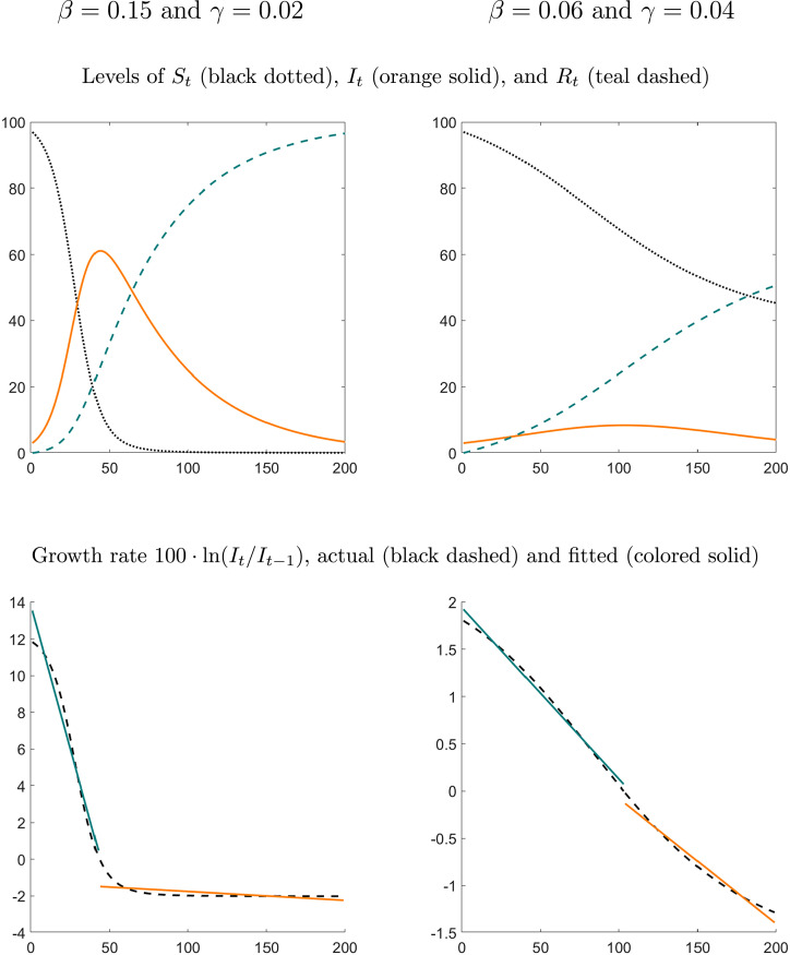
We now simulate the constant-coefficient SIR model in (1) under two different parameterizations for that are unrelated to the current Covid-19 pandemic. The top panels of Fig. 1 depict hypothetical time paths of , , and . The size of the population is normalized to and the outbreak of the disease is triggered by the initial condition .
Fig. 1.
SIR model simulations. Notes: We normalize the size of the population to and set the initial conditions to , , and .
Under the first parameterization (left panels), the transmission rate is very high and the recovery rate is relatively small. This leads to a fast rise in the number of infected individuals, which peaks at in period . After the peak, the number of infections decreases, but more slowly than it increased during the initial outbreak. The bottom left panel shows the growth rate of the infections implied by the SIR model. It is a monotonically decreasing function of time that we approximate by fitting a piecewise linear least-squares regression line with a break point at which is the point in time when the infections peak and the growth rate transitions from being positive to being negative. Under the second parameterization the transmission rate is much lower and the recovery rate is slightly faster. This leads to an almost bell-curve shaped path of infections. While the resulting growth rate of the infections is not exactly a linear function of time , the break at is much less pronounced. While the piecewise-linear regression functions do not fit perfectly, they capture the general time-dependence of the growth-rate path implied by the SIR model. In particular, they allow for a potentially much slower change in the growth rate of infections after the peak.
We use these simulations as a motivation for the subsequent specification of our empirical model.4 This model assumes that the growth rate of infections is a decreasing piecewise-linear function of time with a break when the growth rates cross zero and the infections peak. This deterministic component is augmented by a stochastic component that follows a first-order autoregressive, AR(1), process. We refer to the model as trend-break model. We will revisit a stochastic version of the SIR model that comprises (1), (2) in Section 5.4 where we compare its forecasts to the proposed trend-break model.
3. A Bayesian panel data model
We now describe our empirical model in more detail. We begin with the specification of a regression model for the growth rate of infections in Section 3.1. Our model features location-specific regression coefficients and heteroskedasticity. The prior distribution for the Bayesian analysis is summarized in Section 3.2. Posterior inference is implemented through a Gibbs sampler that is outlined in Section 3.3. Further computational details are provided through replication files on the companion webpage. The algorithm to obtain simulated infection paths from the posterior predictive distribution is outlined in Section 3.4.
3.1. Panel regression specification
We specify a panel data model for infection growth rates , and . We assume that
| (3) |
where is a 2 × 1 vector of heterogeneous coefficients and . is the indicator function that is equal to one if and zero if . The 2 × 1 vector captures the size of the break in the regression coefficients at . The deterministic part of corresponds to the piecewise-linear regression functions fitted to the infection growth paths simulated from the SIR in Fig. 1.
The serially-correlated process generates stochastic deviations from the deterministic path of the infection growth rate. The shocks may capture time variation in the parameters of the SIR model or, alternatively, model misspecification. In Section 2 the break point was given by the peak of the infection path. Abstracting from a potential discontinuity at the kink, we define as
| (4) |
which implies that . Because of the AR(1) process , is not the peak of the observed sample path, nor is it an unbiased or consistent estimate of the period in which the infections peak. For , the model reduces to
| (5) |
Note that the break date is identified in this model even if , because we assume the break occurs when the deterministic component of the growth rate falls below zero.
To construct a likelihood function we define the quasi-difference operator such that . Thus, we can rewrite (3) as follows:
| (6) |
Now let and be the dimension of . The parameters of the panel data model are . Here, we use the notation to denote the sequence . Using this notation, we denote the panel observations by . We will subsequently condition on to initialize conditional likelihood function. Finally, from the growth-rates we can easily recover the level of active infections as
| (7) |
3.2. Prior distribution
To conduct Bayesian inference, we need to specify a prior distribution for . We do so conditional on a vector of hyperparameters that do not enter the likelihood function. Our prior distribution has the following factorization:
| (8) |
where denotes proportionality and is an indicator function that we will use to impose the following sign restrictions on the elements of :
The restriction ensures that the growth rates are falling over time. After the break point the rate of decline decreases (), but stays negative (). In addition we assume that the decrease in the rate of decline is associated with a downward shift, i.e., , of the intercept as shown in the SIR simulation.
Because of the presence of the indicator function the right-hand side of (8) is not a properly normalized density. In view of the indicator function we define the RE distribution of given as
| (9) |
In turn, the marginal prior distribution of the hyperparameters is given by
| (10) |
Building on Liu (2020), we use the following densities in (8) for , , and :
| (11) |
Thus, the vector of hyperparameters is . We decompose . The density is constructed as follows:
| (12) |
The degrees of freedom for the Inverse Wishart distribution are set to
The shape matrix is diagonal with elements
Here, is the sample mean of the time series , , is the cross-sectional sample variance of , , and is a sample average of , and . The matrix is constructed to align the scale of the variance of with the cross-sectional variance of the data, adjusting for the average magnitudes of the regressors that multiply the elements.
To obtain the density , we follow Llera and Beckmann (2016) and let
| (13) |
The parameters need to be chosen by the researcher. We use , , which specifies relatively uninformative priors for hyperparameters and .
3.3. (Approximate) posterior inference
Posterior inference is based on an application of Bayes Theorem. Let denote the likelihood function (for notational convenience we dropped from the conditioning set). Then the posterior density is proportional to
| (14) |
where the prior was given in (8). To generate draws from the posterior distribution we use a Gibbs sampler that iterates over the conditional posterior distributions
| (15) |
The Gibbs sampler generates a sequence of draws , , from the posterior distribution. The implementation of the Gibbs sampler closely follows Liu (2020).
For the Gibbs sampler to be efficient, it is desirable to have a model specification in which it is possible to directly sample from the conditional posterior distributions in (15). Unfortunately, the exact likelihood function leads to a non-standard conditional posterior distribution for because enters the indicator function in (3) through the definition of . Thus, rather than using the exact likelihood function, we will use a limited-information likelihood function of the form
| (16) |
The densities are constructed as follows: Let be some positive number, e.g., three or five time periods. Given a sample we define
If , then it is likely that . On the other hand, if , then it is likely that . Thus, we distinguish two cases:
Case 1: Suppose : we drop observations and define
Because does not enter the likelihood function, its posterior is
Case 2: Suppose : we drop observations and define
Now does enter the likelihood function and its prior gets updated in view of the data.
3.4. Forecasting infection rates
Bayesian forecasts reflect parameter and shock uncertainty. We simulate trajectories of infection growth rates from the posterior predictive distribution using Algorithm 1. The simulated growth rates can be converted into simulated trajectories for active infections using (7).
Algorithm 1 Simulating from the Posterior Predictive Distribution —
- 1.
For
- (a)
Use parameter draw from the posterior distribution: .- (b)
For :
- i.
Compute .- ii.
Generate a sequence of draws , .- iii.
Iterate (6) forward for to obtain .- iv.
Compute , .- 2.
Based on the simulated paths , , compute point, interval, and density forecasts for each period .
4. A simulation experiment
We now conduct a small Monte Carlo experiment that compares the forecasts derived from the panel data model to time-series forecasts generated for each location separately. The experiment shows that in our environment forecasts for locations that experience an outbreak at a later point in time are more accurate than forecasts for locations that have an early outbreak because the early outbreaks facilitate learning about the RE distribution that benefits the forecasts for the remaining locations. The data generating process (DGP) is described in Section 4.1 and the results are summarized in Section 4.2.
4.1. Data generating process
The data generating process (DGP) is given by the trend-break model (3) for the growth rates of infections. For the simulation experiment we assume that the innovations are homoskedastic, i.e., for all . The DGP matches certain aspects of the empirical application in Section 5, but it is more stylized in other dimensions. The time period is a day. The number of locations in our simulation is . We split the locations into two groups: locations experience an early outbreak, starting at , and locations experience a late outbreak, starting at . We refer to these groups as “early” and “late”. For the early group calendar time and event time are identical. For the late group, the event time is calendar time minus (8 weeks).
The parameters of the DGP are summarized in Table 1. The persistence of the growth rates is set to . The dispersion of the parameters is controlled by a vector of means, and a covariance matrix . Both are calibrated to match some stylized facts about the cross-sectional distribution of the country-level data used in Section 5. We then draw the s independently from the distribution. The innovation variance corresponds to a high-density value of the estimated density . We assume that the outbreak starts in each geographical location with .
Table 1.
Parameterization of DGP.
| Persistence: . Innovation variance: . |
| Heterogeneous coefficients: , where |
| Initial infection level: for all . |
We simulate 100 panel data sets of size (, ). To reduce the Monte Carlo noise, for the locations in the late group we are simply replicating the time paths of the early group (shifted by ), rather than generating new paths. For each panel data set, we estimate forecasting models based on a sequence of samples that grow with respect to the time dimension . The first sample comprises the calendar time periods (nine weeks of observations), whereas the last estimation sample ranges from (twenty weeks of observations).
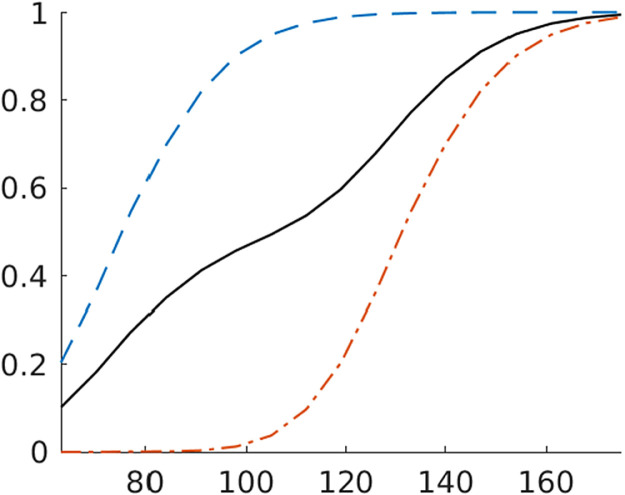
We inspect hairline plots of infection paths , , in calendar time, to confirm that the calibration is reasonable. While the growth rate shocks also generate visible fluctuations in the levels, most infection rate paths have well-defined global peaks. Some of the simulated locations experience multiple waives, but eventually the infection rates fall back to their initial level. Despite the fact that all locations start from the same level of initial infections, there is considerable cross-sectional variation in the level of the infections. There is also heterogeneity in the timing of the peak, which is illustrated in Fig. 2. The figure shows the percentage of locations that have peaked in or prior to period . By construction, infections in the early-group locations tend to peak sooner than in the late-group locations. However, the peak dates in each group are quite dispersed: only 20% of early locations have peaked after 60 days. It takes more than 100 days for the remaining early locations to peak.
Fig. 2.
Empirical distribution of period in which infections peak. Notes: Percentage of locations whose infections have peaked on or before the date specified on the -axis. Blue dashed line is early group, orange dashed-dotted line is late group, and solid black line is all locations.
4.2. Results
Forecasting models. We report results for two forecasting models: (i) the panel data model and (ii) time-series estimates of the trend-break model (3) that ignore the correlation of coefficients across locations.
The panel data model is identical to the one described in Section 3, with the exception that we follow the specification of the DGP and impose homoskedasticity. We use an prior for , where and is sample driven: . To obtain we are computing the variance across all and in the sample, ignoring zero values. The time-series estimates of (3) are obtained from a Bayesian estimation that uses the same prior as the panel data estimation, essentially setting and treating the common parameters and the hyperparameters of the panel model as unit-specific.
Forecast evaluation. Because of the exponential transformation in (7) from growth rates to levels, there is a large degree of cross-sectional heterogeneity among the levels of infection. Locations with larger numbers of infections tend to be associated with larger forecast errors. If we simply average forecast errors or forecast interval lengths across locations, the results will be driven by a few locations with a high level of infections. Therefore, we are standardizing all level-forecast evaluation statistics by the level of infections at the forecast origin, , i.e., we are reporting results for the forecast of .
We will report measures of density and interval forecasting performance below. We do not consider point forecasts because we strongly believe that due to the highly uncertain path of infections during a pandemic it is essential for forecasters to report forecasts that convey the degree of uncertainty in the predictive distribution. The density forecast performance is evaluated based on continuous ranked probability scores (CRPS). The CRPS measures the distance between the cumulative density function associated with a predictive distribution for location at forecast origin and a perfect probability forecast that assigns probability one to the realized :
| (17) |
The CRPS is a proper scoring rule, meaning that it is optimal for the forecaster to truthfully reveal her predictive density. Here could either be a growth rate or a relative level .
For interval forecasts we will report the cross-sectional coverage frequency and the average length separately. As discussed in more detail in Askanazi et al. (2018) aggregating this information based on a common loss function is delicate because the interval length is not scale invariant and many researchers view coverage frequency as having to satisfy an inequality constraint.
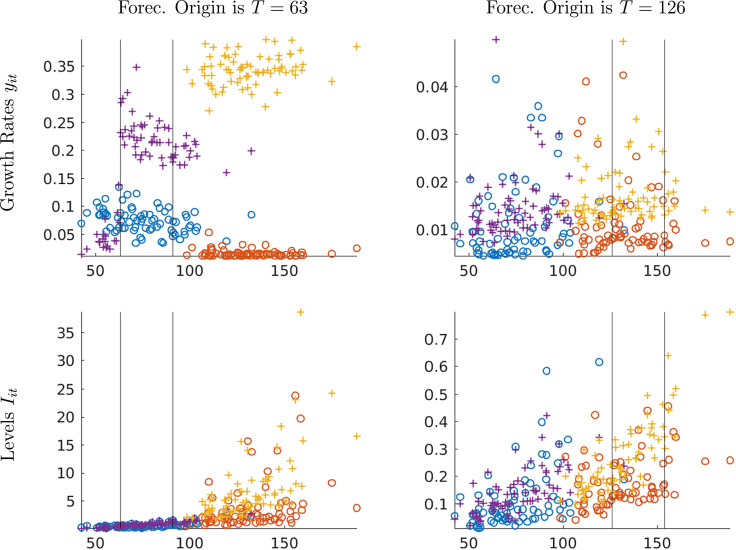
Density forecast accuracy and timing of the infections path. Fig. 3 depicts CRPS values for each location based on a single simulation. The dates on the -axes corresponds to the break point (in calendar time). The forecast horizon in all panels is four weeks, i.e., . The left panels show the scores for the forecast origin in period , whereas the right panels correspond to . The two vertical lines indicate forecast origin and target. The top panels contain results for growth rates and the bottom panels for relative levels . Each panel contains four groups of scores. The circles are scores associated with the forecasts from the panel model, whereas the crosses represent CRPS from time-series regressions. We also distinguish early-group locations (blue and purple) from late-group locations (orange and yellow).
Fig. 3.
Monte Carlo: Density forecast performance (CRPS) for two forecast origins; four-week horizon. Notes: The date on the -axis corresponds to the break point (in calendar time). The two vertical lines indicate forecast origin and target. Panel forecasts: early group is blue circles, late group is orange circles. Time-series forecasts: early group is purple crosses and late group is yellow crosses.(For interpretation of the references to color in this figure legend, the reader is referred to the web version of this article.)
We begin with the top left panel of Fig. 3. In most early-group locations, the infections tend to peak between the forecast origin and the four-week-ahead forecast target . In the late-group locations, the peak occurs after the forecast target date.
For the three important findings emerge. First, the panel forecasts clearly dominate the time-series forecasts. The discrepancy is particularly large for locations in the late group. Second, while for the early group the CRPS based on the panel forecasts seem to be unrelated to the peak date, the accuracy of the time-series forecasts is substantially worse for early-group locations that peak between periods 63 and 91 than it is for locations that peak prior to period 63. Third, the four-week-ahead panel forecasts for the late group are much more accurate than the panel forecasts for the early group.
These findings can be explained as follows: First, in a panel setting, the experience of the early locations allows for relatively precise inference about the RE distribution, which then sharpens the posterior inference for the late locations because the uncertainty about the prior distribution is reduced. Note that the time series dimension for the late group is only 7. Second, due to the structural break in the growth rate at the peak infection level, it is very difficult to predict how quickly the infections will die out after they have peaked. This makes it easier to predict infections for the late group which includes the locations that are still far away from the peak than for the early group in which infection levels are relatively close to the peak.
The top right panel of Fig. 3 indicates that after 18 weeks () the benefit of the panel approach is a lot smaller, both for the early group and the late group. Because more time series information is available to estimate the location-specific parameters, the benefit from using prior information is significantly diminished. The bottom panel of the figure shows CRPS for levels rather than growth rates. The key message remains the same: early on in the pandemic, the panel approach substantially improves forecasts for locations that experience a delayed outbreak, because there is some learning from the locations in which the outbreak occurred early on.
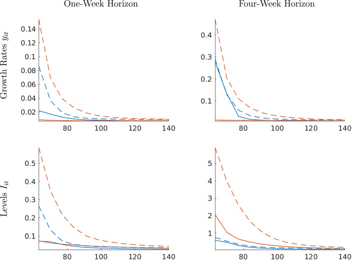
In Fig. 4 we plot the group-specific average CRPS as a function of the forecast origin for one-week-ahead and four-week-ahead forecasts. The main messages from this figure are similar to the messages from Fig. 3, but now the results span a broad range of forecast origins. First, the panel forecasts are (at least weakly) more accurate than the time-series forecasts. However, the accuracy differential vanishes as the time-series dimension of the estimation sample increases over time. Second, the benefit from using a panel approach is more pronounced for the locations that experience a late outbreak than those that experience an early outbreak.
Fig. 4.
Monte Carlo: Density forecast performance (CRPS). Notes: Panel forecasts are solid and time-series forecasts are dashed. Blue lines correspond to early-group averages and orange lines to late-group averages.(For interpretation of the references to color in this figure legend, the reader is referred to the web version of this article.)
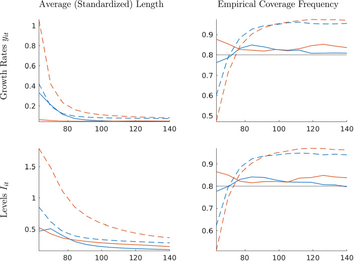
Interval forecast accuracy. Finally, we report results on the interval forecast performance for infection growth rates and levels in Fig. 5. The interval forecasts are 80% posterior probability intervals (equal-tail probability). The left panels summarize the average length of the forecast intervals by location group and forecast method. The right panels depict the empirical coverage frequencies. The empirical coverage frequencies can be compared to the nominal credible level of the interval forecasts. However, this comparison is delicate. While in finite samples the two objects tend to differ, one can show that if the posterior distribution of concentrates around a limit point as , then under suitable regularity conditions, the discrepancy between the empirical coverage frequency and the credible level will vanish.5
Fig. 5.
Monte Carlo: Interval forecast performance; one-week horizon. Notes: Average length and empirical coverage frequency for 80% posterior probability intervals. Panel forecasts are solid and time-series forecasts are dashed. Blue lines correspond to early-group averages and orange lines to late-group averages.(For interpretation of the references to color in this figure legend, the reader is referred to the web version of this article.)
The panel interval forecasts have an empirical coverage frequency that is close to their posterior credible level of 80%. The coverage frequency is fairly insensitive to the forecast origin and the data transformation (growth rates versus levels). The left panels indicate that for the late-group, the average standardized length for the panel interval forecasts is substantially shorter (both for growth rates and levels) than for time-series forecasts. For the locations that experience an early outbreak, the average lengths of panel and time-series interval forecasts are quite similar. For the time-series forecasts there is a substantial mismatch between coverage level and empirical coverage probability. Early on, for , the coverage frequency is substantially less than 80%, whereas after it is around 95%. Because the empirical coverage frequency of the panel forecasts approximately matches the nominal credible level, the panel forecasts are preferable for all forecast origins in this experiment.
5. Empirical analysis
We apply the panel forecasting techniques to country/region-level data on active Covid-19 infections. The data set used in the empirical analysis is described in Section 5.1. We discuss the posterior estimates for the 2020-04-18 forecast origin in Section 5.2. In Section 5.3 we inspect the density forecasts for three countries at different stages of the pandemic: South Korea, Germany, and the U.S. Finally, in Section 5.4 we evaluate the Covid-19 infection forecasts over a longer period of time, comparing our panel model to time-series estimates of the trend-break model and a stylized SIR model. Since we completed the first draft of this paper in May 2020, we have been publishing real-time forecasts at a weekly frequency online at https://laurayuliu.com/covid19-panel-forecast/.
5.1. Data
The data set is obtained from CSSE at Johns Hopkins University.6 We define the total number of active infections in location and period as the number of confirmed cases minus the number of recovered cases and deaths. The goal of our modeling effort is to predict the number of active infections as recorded in the CSSE data set. The data set has some limitations. Infections are measured with error because there is evidence that a significant number of infected individuals are asymptomatic and hence not captured in the official statistics. Determining the precise number of Covid-19 related deaths is non-trivial (dying with versus dying of Covid-19) and counts of the number of recovered individuals are often inaccurate. However, improving the data quality is beyond the scope of this paper.
Throughout our study we use country-level aggregates. The time period corresponds to a day and we fit our model to one-sided three-day rolling averages to smooth out noise generate by the timing of the reporting. In a slight abuse of notation, the time subscript in (3) is meant to be event time and hence is specific on the location . The event time is initialized once the number of confirmed cases in a location reaches 100.7 For each location, we let the time series of infections end at the same calendar time. As a result, the panel is unbalanced.
Our empirical analysis is based on a cross-section of over 100 countries/regions. We start out from 185 locations and eliminate a subset of locations according to the following rules: (i) we eliminate locations that have not reached 100 active infections. (ii) We eliminate locations for which . This guarantees that we have at least one observation in the limited-information likelihood function to extract information about . (iii) For each location we regress the growth rates from period to on a time trend and an intercept and eliminate locations where the OLS estimate of the time-trend coefficient is positive because the SIR model implies a decreasing growth rate. The resulting cross-sectional dimension of our panel is around 110 for early forecast origins and around 150 for late forecast origins.
5.2. Parameter estimates for 2020-04-18
Before discussing the forecasts, we will examine the parameter estimates for one of the early samples, namely 2020-04-18.
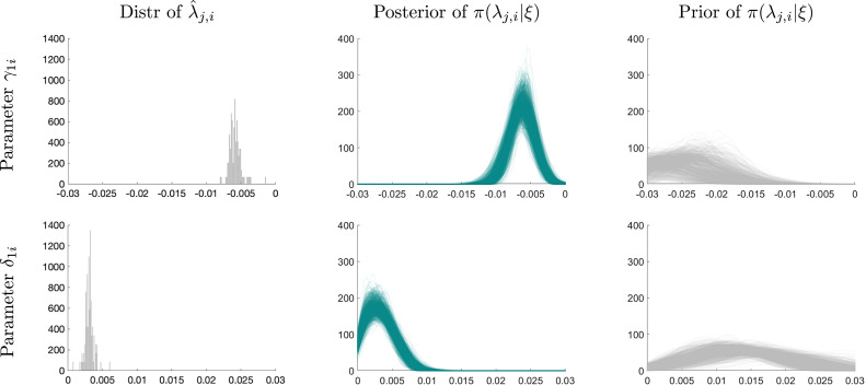
Heterogeneous slope coefficients. Our Gibbs sampler generates draws from the joint posterior of . We begin with a discussion of the estimates of and , which affect the speed at which the growth rates are expected to change on a daily basis. measures the average daily decline in the growth rate of active infections. For instance, suppose the at the beginning of the outbreak, in event time , the growth rate , i.e., approximately 20%. A value of implies that, on average, the growth rate declines by 0.02, meaning that after 10 days it is expected to reach zero and turn negative subsequently. A positive value of implies that after the growth rate becomes negative, its decline is reduced (in absolute value) to .
In the first column of Fig. 6 we plot the cross-sectional distributions of posterior mean estimates and . Almost all of the ’s are in the interval . The cross-sectional distribution peaks at approximately 0.006. In absolute values, the estimates of are roughly half the size of the ’s, meaning that the recovery after the infections have peaked will take considerably longer than the rise to the peak.
Fig. 6.
Heterogeneous coefficients estimates and random effects distributions. Notes: Point estimator is posterior mean of or , respectively.
Random effects distribution. An important component of our model is the RE distribution defined in (9). Prior and posterior uncertainty with respect to the hyperparameters generate uncertainty about the RE distribution. In the remaining panels of Fig. 6 we plot draw from the posterior (center column) and prior (right column) distribution of the RE density . Each draw is represented by a hairline. Because the normalization constant of is difficult to compute due to the truncation of a joint Normal distribution, we show kernel density estimates obtained from draws from .
The RE densities are drawn from the posterior approximately peak around values of and for which the histograms on the left are peaking. Thus, the estimates of the densities cohere with the estimates of the heterogeneous coefficients. The precise relationship between the hairlines that represent draws from the distribution of the RE densities and the posterior point estimates are discussed in more detail in Liu et al. (2019). The RE densities are generally more diffuse than the distributions of the point estimates represented by the histograms because the RE densities can be viewed as priors of whereas the point estimates combine information from these priors and the time series .
The RE densities drawn from the prior distribution of are fairly flat. Because of the truncation, the means implied by the RE densities for are negative, whereas the means implied by the densities for are positive. The priors for the RE densities are dependent on the sample because the overall prior is indexed by data-dependent tuning parameters; see Section 3.2.
The remaining parameters. Our posterior sampler also generates estimates for the homogeneous autoregressive coefficient . The posterior mean is . Point estimates of range from approximately 0.02 to 0.06. The cross-sectional distribution of these estimates is skewed to right with a few estimates exceeding 0.07.
Implied regression functions. After examining the cross-sectional distribution of the and estimates, we will now inspect the implied regression functions that capture the deterministic component of the infection growth rates for three specific countries: China, South Korea, and Germany. These three countries experienced the outbreak at different points in time. The posterior median estimates from which the regression lines depicted in Fig. 7 are constructed, reflect the prior information from the RE distributions depicted in Fig. 6 and the time series information for each country. By construction, the regression lines are piecewise linear, and the break occurs at the point in time when the deterministic component implies a zero growth rate. The fitted regression line for South Korea reflects a fair amount of shrinkage induced by the prior distribution, because the initial rapid decline in the growth rate is unusual according to the estimated cross-sectional RE distribution.
Fig. 7.
Fitted regression lines for daily infection growth rates.
5.3. Predictive densities
We now turn to density forecasts generated from the estimated panel data model. For now, we will focus on the early stage of the pandemic. We use Algorithm 1 to simulate trajectories of infection growth rates which, conditional on observations of the initial levels , we convert into stocks of active infections. For each forecast horizon we use the values and , to approximate the predictive density. Strictly speaking, we are not reporting complete predictive densities. Instead, we plot medians and construct equal-tail-probability bands that capture the range between the 20%–80% and 10%–90% quantiles. The wider the bands, the greater the uncertainty.
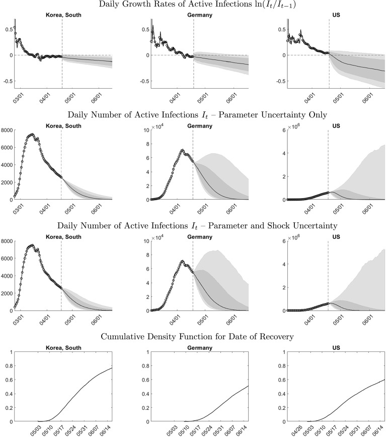
Fig. 8 shows density forecasts over 60 days for the growth rate, the level of active infections, and the recovery date in South Korea, Germany, and the U.S. based on 2020-04-18 data.8 The forecast origin is indicated by the vertical dashed line. At the forecast origin, the three countries are at different stages of the epidemic. In South Korea, the level of infections is 67 percent below its peak value. Germany has barely moved beyond the peak and the U.S. is still far away from its peak. Prior to the forecast origin we show the actual values and in-sample fitted values.9
Fig. 8.
2020-04-18 forecasts for South Korea, Germany, and the U.S. Notes: Rows 1 to 3: The vertical lines indicate the forecast origin. The circles indicate actual infections. The solid lines prior to the forecast origin represent in-sample one-step-ahead forecasts. The solid lines after the forecast origin represent medians of the posterior predictive distribution. The gray shaded bands indicate the 20%–80% (dark) and 10%–90% (light) interquantile ranges of the posterior predictive distribution. Bottom row: cumulative density function (associated with posterior predictive distribution) of date of recovery defined as such that .
The panels in the first row of Fig. 8 show forecasts for the growth rate of active infections. At the forecast origin, the actual growth rates for South Korean and Germany are negative, whereas the growth rate for the U.S. is positive. The median forecast is driven by the deterministic trend component in our model for ; see (3) and Fig. 7. The bands reflect both parameter uncertainty and stochastic fluctuations around the trend component generated by the autoregressive process .
The width of the bands is the smallest for South Korea and the largest for the U.S. Two factors potentially contribute to the wider bands for the U.S.: shock uncertainty and parameter uncertainty. Shock uncertainty is not the driving factor. The estimated shock standard deviations for the two countries are very similar: 0.032 for South Korea and 0.035 for the U.S. Instead, parameter uncertainty is the culprit. Recall that at the peak, the parameters of the deterministic component of our model shift by . Because the growth rate in the U.S. has not yet crossed zero and the country has not reached the peak, there are no observations available yet to estimate , which increases the contribution of parameter uncertainty to the predictive distribution.
The second and third rows of Fig. 8 depict predictions for the daily level of active infections. The path of active infections broadly resembles the paths simulated with the SIR model in Section 2. The rise of infections during the outbreak tends to be faster than the subsequent decline, which is a feature that is captured by the break in the conditional mean function of our model for the infection growth rate in (3). The difference between the bands depicted in the second and third rows is that the former reflects parameter uncertainty only (we set future shocks equal to zero), whereas the latter reflects parameter and shock uncertainty. In the case of Germany, shock uncertainty increases the width of the bands by approximately 30%.
Due to the exponential transformation that is used to recover the levels, the predictive densities are highly skewed and exhibit a large upside risk. This is particularly evident for the U.S. The growth rate prediction in the first row indicates that there is an approximately 20% probability of a positive infection growth rate throughout April and at least a 10% probability until the middle of June. Converted into levels, temporarily positive growth rates of infections can generate a rise of infections from less than one million in April to more than five million two months later.
In the bottom row of Fig. 8 we plot cumulative density function for the date of recovery, which we define as the first date when the infections fall below the initial level . The density function is calculated by examining each of the future trajectories for generated by Algorithm 1. For South Korea the probability that the infection rate will fall below over the two month period is close to 80%, whereas for Germany and the U.S. the probability is approximately 50% and 60%, respectively.
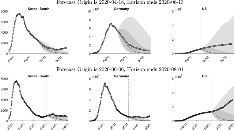
In Fig. 9 we overlay eight weeks of actual infections onto density forecasts generated from the 2020-04-18 (top panels) and 2020-06-06 (bottom panels) samples. The forecasts in the top row are identical to the ones reported in Fig. 8. Forecasts for South Korea and Germany are remarkably accurate. Over a two-week horizon the actuals are very close to the median prediction. Subsequently the actual infection level falls less quickly than predicted by the model. For Germany the actual path remains with the 60% credible band whereas for South Korea it moves outside of the narrow 80% credible band after six weeks.
Fig. 9.
Interval forecasts and actuals. Notes: The vertical lines indicate the forecast origins. The circles indicate actual infections. The solid lines prior to the forecast origin represent in-sample one-step-ahead forecasts. The solid lines after the forecast origin represent medians of the posterior predictive distribution. The gray shaded bands indicate the 20%–80% (dark) and 10%–90% (light) interquantile ranges of the posterior predictive distribution.
For the U.S., according to the median of the predictive distribution, infection levels should fall shortly after the forecast origin. However, this fall does not occur. Instead the level of active infections is steadily rising. Because the U.S. density forecast exhibits a significant tail risk, the actual infections remain within the 60% band until early May and within the very wide 80% band throughout the eight-week forecast period.
The second row of Fig. 9 depicts forecasts based on the 2020-06-06 sample. Compared to the middle of April, the infection levels in South Korea and Germany have fallen further and our model predicts a continued decline. This prediction turned out overly optimistic as the infection levels in both countries remained high and even increased temporarily. The actuals are generally outside of the 60% credible band and are barely covered by the upper edge of the 80% band. For the U.S. the posterior median prediction of our model is a fairly quick recovery from the pandemic. However, the 80% band still shows a substantial upside risk of more than four million infections at the beginning of August. The actual level of infections in the U.S. continues to rise. By the end of June it has climbed outside of the 60% credible band but stays well within the 80% band.
5.4. Forecast evaluation
We now turn to a more systematic evaluation of the forecasts and will assess the accuracy of density and interval forecasts represented by the bands in Fig. 8, Fig. 9. For reasons previously discussed in Section 4.2, we standardize future infections by the level of infections at the forecast origin. A closer inspection of the forecasts for more than 100 countries/regions reveals that the long-run forecasting performance is not particularly good. This is not just a feature of our panel trend-break model, but also a feature of other epidemiological models such as the SIR model for which we will report results below. Thus, in this section we will focus on one-week and four-week ahead forecasts and not report results for an eight-week horizon.
Alternative models. In addition to the panel model forecasts, we consider two alternative forecasts. First, as in Section 4, we generate time-series forecasts based on the trend-break model (3) for each location. Second, we estimate a version of the simple SIR in (1) with time-varying parameters and . Notice, that by rewriting (1) we can express and directly as a function of the observables (here we are omitting subscripts)10 :
| (18) |
This allows us to estimate the AR(1) law of motion in (2) for each country using Bayesian techniques. The AR(1) models are then used to simulate trajectories from the posterior predictive distribution.11 For each parameter sequence, we iterate the SIR model (1) forward to obtain a predictive distribution of the active infections.
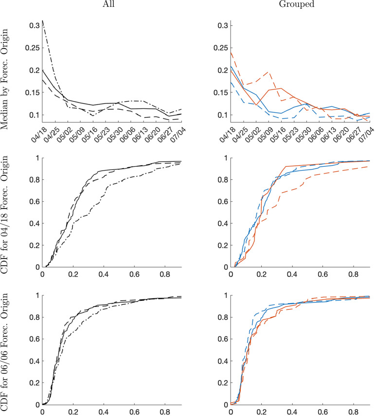
Density forecast accuracy. Fig. 10 summarizes the one-week-ahead density forecasting performance for once-a-week forecast origins starting on 2020-04-18 and ending on 2020-07-04. For each location, we compute the probability score . The top row shows the cross-sectional median as a function of the forecast origin, whereas the center and the bottom row show the cross-sectional empirical distribution for two forecast origins: 2020-04-18 and 2020-06-06.
Fig. 10.
CRPS, one-week horizon. Notes: Left column panels: solid is panel, dashed is country-level, and dashed-dotted is SIR. Right column panels: solid is panel, dashed is country-level. Blue lines correspond to early group and orange lines to late group.(For interpretation of the references to color in this figure legend, the reader is referred to the web version of this article.)
The panels in the left column of Fig. 10 cover all locations, whereas the panels in the right column distinguish between early-group and late-group locations. The early group comprises locations that experienced more than 100 infections before 2020-03-28. The remaining locations are assigned to the late group. The groups evolve over time as more locations experience Covid-19 outbreaks and pass our sample selection criteria; see Section 5.1. For the 2020-04-18 sample the early group has 84 and the late group has 25 locations. For the 2020-06-06 the sample sizes are 87 and 58, respectively.
The top row of Fig. 10 shows that as time progresses and information accumulates, forecast performance improves for all methods in general. Across all locations (top left panel), the time series forecasts from the trend-break model are slightly more accurate than the panel forecasts as indicated by the lower median CRPS. However, comparing the empirical distribution functions for the 2020-04-18 and 2020-06-06 origins (center left and bottom left panels), the overall difference in performance across units is fairly small.
The panels in the right column of Fig. 10 distinguish between locations that experienced the Covid-19 outbreak at an early stage and locations that were hit by the pandemic at a later stage. The key result is that for forecast origins dated 2020-05-09 or earlier, the panel forecasts for the late group are more accurate than the time series forecasts from the trend-break model. This result confirms the basic intuition that the panel approach can be advantageous during a slowly spreading pandemic because the experience of the early-group countries can sharpen inference on the RE distribution for the latter countries. Unfortunately, because the time series approach dominates the panel approach for the early countries, in the aggregate there is no clear advantage to the panel analysis in our data set.
The left panels of Fig. 10 also contain the CRPS for the stylized SIR model. Except for the forecast origins in the month of May, the SIR forecasts of the level of infections are dominated by the panel and time-series forecasts from the trend-break model. However, as time progresses the accuracy differentials across models decreases. To understand the difference between the trend-break model and SIR model forecasts we also examined the accuracy of the infection growth forecasts. It turns out, that in terms of growth rates the SIR model performs quite well. The key difference between the SIR and the trend-break forecasts is that the former are downward biased for the early dates, whereas the latter have an upward bias. Over time, the bias of the forecasts converges. A negative bias means that the SIR model overpredicts the growth rate, which can lead to potentially large errors in the level forecast, in particular if predicted growth rates exceed one and imply explosive behavior.
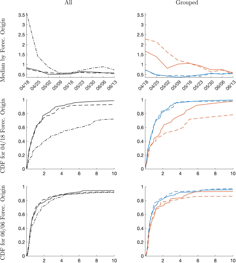
Fig. 11 shows results for four-week-ahead density forecasts. Qualitatively, they are very similar to the one-week-ahead forecasts, but there are some important quantitative differences. First, in the early stage of the pandemic the SIR model forecasts are now substantially worse than the forecasts from the trend-break model. Second, while the median CRPS from the panel model and the time series model are essentially identical for all forecast horizons, the empirical distribution for the 2020-04-18 origin indicates that in the right tail of the CRPS distribution, the panel forecasts dominate the time-series forecasts. This performance difference is driven by the late group, which can be seen from the panels in the right column and vanishes in the middle of May as more time series information becomes available for both groups.
Fig. 11.
CRPS, four-week horizon. Notes: Left column panels: solid is panel, dashed is country-level, and dashed-dotted is SIR. Right column panels: solid is panel, dashed is country-level. Blue lines correspond to early group and orange lines to late group.(For interpretation of the references to color in this figure legend, the reader is referred to the web version of this article.)
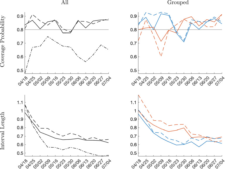
Interval forecast accuracy. We are considering interval forecasts with a nominal coverage probability of 80%. The intervals are constructed as equal-tail probability intervals from the posterior predictive distribution. Results for the one-week forecast horizon are presented in Fig. 12. The coverage frequencies for the trend-break model forecasts (panel and time series) are fairly close to the nominal level of 80%. The coverage frequency of the SIR model interval forecast, on the other hand, is substantially lower than the nominal level. The panel data forecasts have a smaller average length than the individual-level forecasts for both groups and in the aggregate. Thus, on balance, in terms of interval forecasting, the panel approach comes out slightly ahead. Finally, the bottom right panel shows that the interval forecasts for the late group are generally wider than for the early group. The additional uncertainty is caused by the difficulty of predicting the change in infection growth rates around the peak.
Fig. 12.
Interval forecast performance, one-week horizon. Notes: The nominal coverage probability is 80%. Left column panels: solid is panel, dashed is country-level, and dashed-dotted is SIR. Right column panels: solid is panel, dashed is country-level. Blue lines correspond to early group and orange lines to late group.(For interpretation of the references to color in this figure legend, the reader is referred to the web version of this article.)
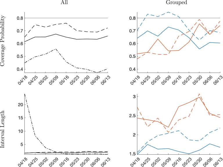
Fig. 13 displays results for a four-week horizon. Over this longer horizon, the coverage frequency is generally poor. As for the shorter horizon, the SIR model interval forecasts are substantially worse in terms of coverage frequency and interval length than the panel and time-series forecasts from the trend-break model.
Fig. 13.
Interval forecast performance, four-week horizon. Notes: Left column panels: solid is panel, dashed is country-level, and dashed-dotted is SIR. Right column panels: solid is panel, dashed is country-level. Blue lines correspond to early group and orange lines to late group.(For interpretation of the references to color in this figure legend, the reader is referred to the web version of this article.)
6. Conclusion
We adopted a panel forecasting model initially developed for applications in economics to forecast active Covid-19 infections. A key feature of our model is that it exploits the experience of countries/regions in which the epidemic occurred early on, to sharpen forecasts and parameter estimates for locations in which the outbreak took place later in time. At the core of our model is a specification that assumes that the growth rate of active infections can be represented by autoregressive fluctuations around a downward sloping deterministic trend function with a break. Our specification is inspired by infection dynamics generated from a simple SIR model.
According to our model, there is a lot of uncertainty about the evolution of infection rates, due to parameter uncertainty and the realization of future shocks. Moreover, due to the inherent nonlinearities and exponential transformations, predictive densities for the level of infections are highly skewed and exhibit substantial upside risk. Consequently, it is important to report density or interval forecasts, rather than point forecasts.
A natural extension of our model is to allow for additional, data-determined breaks in the deterministic trend function as the pandemic unfolds and countries/regions are adopting new policies that accelerate or decelerate the spread of the virus and as more and more people become resistant to the infection. It is also worthwhile to link the heterogeneous coefficient estimates (or transformations thereof) to location-specific variables that measure social norms and policies to fight the pandemic. This could be done in a second step through ex-post regressions with the heterogeneous coefficient estimates as left-hand-side variables or, more elegantly, in a correlated RE framework.
Footnotes
We thank Elie Tamer (co-editor), an anonymous referee, Graham Elliott, and participants at the 26th IIF workshop on Economic Forecasting in Times of COVID-19, the NBER-NSF Seminar on Bayesian Inference in Econometrics and Statistics, and the FRB Philadelphia Conference on Real Time Data Analysis for helpful comments and suggestions. We also thank the Johns Hopkins University Center for Systems Science and Engineering for making Covid-19 data publicly available on GitHub and Evan Chan for his help in developing the website on which we publish our forecasts. Moon and Schorfheide gratefully acknowledge financial support from the National Science Foundation, USA under Grants SES 1625586 and SES 1851634, respectively. Moon thanks Dr. S. Kim, Dr. C. Moon, and Dr. H. Song of GemVax & KAEL for helpful conversations on Covid-19 related topics.
As opposed to micro-simulation or agent-based models.
For forecasts generated directly from an enriched version of the SIR model see, for instance, Fernandez-Villaverde and Jones (2020).
See Liu et al. (2019) for a more detailed discussion.
In calendar time, let . Using , we take log differences to compute growth rates , , . In the estimation we need one growth rate observation to initialize lags. Thus, in event time, period corresponds to .
Compared to Fig. 7, we replaced China by the U.S. because in mid-April the reported levels of Covid-19 infections in China had already fallen from 58,000 to 1600.
The fitted values are generated as follows: for each draw from the posterior distribution, we generate a one-step-ahead in-sample prediction for each country/region. Then we compute the median across these in-sample predictions for each location.
The following additional variables are obtained from the JHU CSSE dataset: is the total population of each country. is computed as - — recovered cases–deaths.
Based on the specification of the SIR model, we let and , for all .
Supplementary material related to this article can be found online at https://doi.org/10.1016/j.jeconom.2020.08.010.
Appendix A. Supplementary data
The following is the Supplementary material related to this article.
Alternative Covid-19 Forecasts.
References
- Askanazi R., Diebold F.X., Schorfheide F., Shin M. On the comparison of interval forecasts. J. Time Series Anal. 2018;39(6):953–965. [Google Scholar]
- Avery C., Bossert W., Clark A.T., Ellison G., Fisher Ellison S. Covid Economics, Vol. 12. CEPR Press; 2020. Policy implications of models of the spread of coronavirus: Perspectives and opportunities for economists; pp. 21–68. [Google Scholar]
- Bertozzi A.L., Franco E., Mohler G., Short M.B., Sledge D. 2020. The challenges of modeling and forecasting the spread of COVID-19. arXiv:2004.0474v1. [DOI] [PMC free article] [PubMed] [Google Scholar]
- de Boor C. Birkhäuser Verlag; Basel: 1990. Splinefunktionen, Lectures in Mathematrics, ETH Zürich. [Google Scholar]
- Brown L.D., Greenshtein E. Nonparametric empirical Bayes and compound decision approaches to estimation of a high-dimensional vector of normal means. Ann. Statist. 2009:1685–1704. [Google Scholar]
- Eichenbaum M.S., Rebelo S., Trabandt M. 2020. The Macroeconomics of Epidemics: NBER Working Paper, 26882. [Google Scholar]
- Fernandez-Villaverde J., Jones C.I. University of Pennsylvania; 2020. Estimating and Simulating a SIRD Model of COVID-19 for Many Countries, States, and Cities. Manuscript. [DOI] [PMC free article] [PubMed] [Google Scholar]
- Glover A., Heathcote J., Krueger D., Rios-Rull J.-V. Covid Economics, Vol. 6. CEPR Press; 2020. Health versus wealth: On the distributional effects of controlling a pandemic; pp. 22–64. [Google Scholar]
- Gu J., Koenker R. Empirical Bayesball remixed: Empirical Bayes methods for longitudinal data. J. Appl. Econ. 2017;32(3):575–599. [Google Scholar]
- Gu J., Koenker R. Unobserved heterogeneity in income dynamics: An empirical Bayes perspective. J. Bus. Econom. Statist. 2017;35(1):1–16. [Google Scholar]
- Haavelmo T. The probability approach in econometrics. Econometrica. 1944;12:1–115. [Google Scholar]
- Ho P., Lubik T.A., Matthes C. Indiana University; 2020. Going Viral: Forecasting the Coronavirus Pandemic Across the U.S. Manuscript. [Google Scholar]
- Kermack W.O., McKendrick A.G. A contribution to the mathematical theory of epidemics. Proc. R. Soc. Lond. Ser. A. 1927;115(772):700–721. [Google Scholar]
- Krueger D., Uhlig H., Xie T. University of Pennsylvania; 2020. Macroeconomic Dynamics and Reallocation in an Epidemic. Manuscript. [Google Scholar]
- Larson W.D., Sinclair T.M. 2020. Nowcasting unemployment insurance claims in the time of COVID-19. [DOI] [PMC free article] [PubMed] [Google Scholar]
- Li S., Linton O. University of Cambridge; 2020. When Will the Covid-19 Pandemic Peak? Manuscript. [Google Scholar]
- Liu L. 2020. Density forecasts in panel data models: A semiparametric Bayesian perspective. arXiv preprint arXiv:1805.04178. [Google Scholar]
- Liu L., Moon H.R., Schorfheide F. 2019. Forecasting with a Panel Tobit Models: NBER Working Paper, 26569. [Google Scholar]
- Liu L., Moon H.R., Schorfheide F. Forecasting with dynamic panel data models. Econometrica. 2020;88(1):171–201. [Google Scholar]
- Llera A., Beckmann C. 2016. Estimating an inverse gamma distribution. arXiv preprint arXiv:1605.01019. [Google Scholar]
- Murray C.J. 2020. Forecasting the impact of the first wave of the COVID-19 pandemic on hospital demand and deaths for the USA and European economic area countries. medRxiv. [DOI] [Google Scholar]
- Stock J.H. Covid Economics, Vol. 3. CEPR Press; 2020. Dealing with data gaps; pp. 1–11. [Google Scholar]
Associated Data
This section collects any data citations, data availability statements, or supplementary materials included in this article.
Supplementary Materials
Alternative Covid-19 Forecasts.


