Abstract
In this paper, we present a novel method, called four-dimensional convolutional recurrent neural network, which integrating frequency, spatial and temporal information of multichannel EEG signals explicitly to improve EEG-based emotion recognition accuracy. First, to maintain these three kinds of information of EEG, we transform the differential entropy features from different channels into 4D structures to train the deep model. Then, we introduce CRNN model, which is combined by convolutional neural network (CNN) and recurrent neural network with long short term memory (LSTM) cell. CNN is used to learn frequency and spatial information from each temporal slice of 4D inputs, and LSTM is used to extract temporal dependence from CNN outputs. The output of the last node of LSTM performs classification. Our model achieves state-of-the-art performance both on SEED and DEAP datasets under intra-subject splitting. The experimental results demonstrate the effectiveness of integrating frequency, spatial and temporal information of EEG for emotion recognition.
Keywords: EEG, Emotion recognition, 4D data, Convolutional recurrent neural network
Introduction
Emotion recognition has received increasing attention in the field of affective computing in recent years, due to its potential applications in human–machine interaction (HMI) (Fiorini et al. 2020; Cowie et al. 2001), diseases evaluation (Figueiredo et al. 2019; Bamdad et al. 2015; Vansteensel and Jarosiewicz 2020) and driving fatigue detection (Kong et al. 2017; Zeng et al. 2018, 2019b), and mental workload estimation (Blankertz et al. 2016; Aricò et al. 2019; Cartocci et al. 2015). Emotion recognition methods could be categorized into two major classes, one is based on non-physiological signals [e.g., facial expression and speech (Yan et al. 2016; Zhang et al. 2019)] and another is based on physiological signals [e.g., electroencephalography (EEG) and electrocardiography (ECG) (Chen et al. 2015; Zheng et al. 2017; Hsu et al. 2017)]. EEG is characterized by noninvasive, portability, reliability, and small cost. It has been widely used in the field of brain–computer interfaces (BCIs) (Pfurtscheller et al. 2010; Aricò et al. 2018, 2020), which establishing a direct communication channel between human beings and computers. Recently, enhancing BCI by taking advantage of the information of the user’s emotional states from EEG has gained more and more attention, which termed as affective brain–computer interface (aBCI) (Mühl et al. 2014; Garcia-Molina et al. 2013; Goshvarpour and Goshvarpour 2019). The goal of aBCI is to make machines have the ability to perceive, understand, and regulate emotions, and the key problem of it is to recognize emotion from EEG.
From traditional hand-crafted features based methods to deep learning methods, considerable progress has been made in the community of EEG-based emotion recognition (Alarcão and Fonseca 2017; Garcia-Molina et al. 2013; Mühl et al. 2014; Zeng et al. 2019a). Before the surge of deep learning, there are three kinds of features dominant in EEG emotion recognition, including time domain features (Frantzidis et al. 2010; Ansari-Asl et al. 2007; Kroupi et al. 2011), frequency domain features (Li and Lu 2009; Rozgić et al. 2013; Reuderink et al. 2013) and time–frequency domain features (Akin 2002; Murugappan et al. 2010). However, these features are usually low-level and designed by specific purposes, thus they may not be discriminative enough to detect emotions. Hence, deep learning algorithms are developed, which can learn high-level features automatically from data (He et al. 2016; Krizhevsky et al. 2012). Zheng and Lu (2015) introduced deep belief networks (DBNs) to investigate the critical frequency bands and channels of EEG for emotion recognition. Song et al. (2018) proposed dynamical graph convolutional neural networks (DGCNN) to perform EEG emotion classification. Ma et al. (2019) designed a multimodal residual LSTM (MMResLSTM) network for emotion recognition. All of those deep models achieve better performance than shallow models.
However, for the EEG representation building based on deep learning, there are still some challenges to be solved and one of them is how to fuse more useful information of EEG signals to perform emotion recognition better. First, in the past decade, many researchers investigated the relationship between frequency bands of EEG and emotion types. They not only found that there were four frequency bands strongly associated with emotion, including Theta (: 4–7 Hz), Alpha (: 8–13 Hz), Beta (: 14–30 Hz), and Gamma (: 31+Hz), but also suggested that combining all these four bands was better than any individual band when classifying emotions (Zheng and Lu 2015; Yang et al. 2018a). Second, some researchers extracted spatial features of EEG, which inspired by EEG devices that have multiple electrodes place different positions of the cerebral cortex to collect electric potentials. They explored intrinsic information contained in the positional relationship among electrodes to improve the performance of emotion recognition. For example, Zhang et al. (2018) proposed a quad-directional recurrent neural network (RNN) based method to capture long-distance spatial dependencies among electrodes at a single moment. However, they only used four scanning orders of electrodes which may be unable to cover the complex relationship between different electrodes. Li et al. (2018) constructed data from 62 electrodes as two-dimensional (2D) spare maps to train the deep learning model. Third, some researchers found that not only the spatial information of multiple electrodes at a temporal slice is critical for emotion recognition, but also the contextual dependencies among temporal slices. For instance, Wang et al. (2018) devised EmotioNet constructed by three-dimensional (3D) CNN to simultaneously extract features in spatial and temporal domains. Hochreiter and Schmidhuber (1997) designed a parallel convolutional recurrent neural network (PCRNN) which extracts spatial and temporal features from EEG by CNN and RNN with Long Short-Term Memory (LSTM) cells respectively, and then concatenates the outputs of CNN and LSTM directly to make classification (Yang et al. 2018b). From the above, it can be observed that frequency, spatial and temporal features of EEG signals are all important for emotion recognition. However, these methods only consider one or two of these three kinds of features. To the best of our knowledge, there is little literature available that integrating frequency, spatial and temporal information simultaneously in EEG-based emotion recognition.
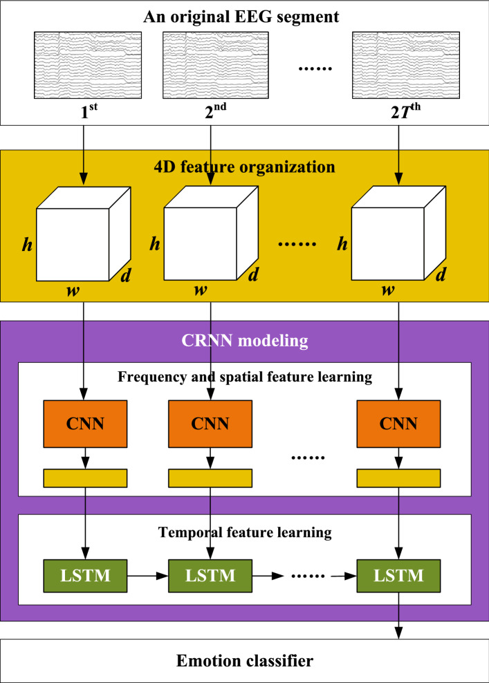
To address this issue, a new segment-level EEG-based emotion recognition method is proposed in this paper, called four-dimensional convolutional recurrent neural network (4D-CRNN), as illustrated in Fig. 1. Our method aims to effectively and efficiently integrate frequency, spatial and temporal information of EEG signals to recognition emotions. At first, a 4D feature structure is built, which explicitly organizing these three kinds of information of EEG. Then CRNN model is introduced, which is combined by CNN and LSTM. Different from PCRNN, we conduct a deeper fusion of CNN and LSTM modules. Specifically, CNN is used to learn frequency and spatial representation for each temporal slice in 4D structures. RNN with LSTM cells takes the outputs of CNN as input and extracts the temporal dependency between slices.
Fig. 1.
An overview of the proposed EEG-based emotion recognition framework using 4D-CRNN
In summary, our contributions include: (a) We propose a 4D feature structure, which contains frequency, spatial and temporal information of EEG explicitly. We also design a deep model to simultaneously learn these three kinds of information from the 4D structure for EEG-based emotion recognition. The method is dubbed 4D-CRNN; (b) The experimental results of 4D-CRNN demonstrate that integrating different frequency bands, effective electrodes relationship and appropriate length of segments significantly improves classification performance; (c) 4D-CRNN achieves the state-of-the-art performance both on SEED (Zheng and Lu 2015) and DEAP (Koelstra et al. 2012) datasets.
In the remainder of this paper, we describe our proposed method in “Method” section. In “Experiment” section, the datasets, experiment setting, results and discussion are presented. Conclusions are given in “Conclusion” section.
Method
Figure 1 shows the framework of 4D-CRNN for EEG-based emotion recognition. It includes three parts: 4D feature organization, CRNN modeling and classifier. The details of each part will be introduced in sequence.
4D feature organization
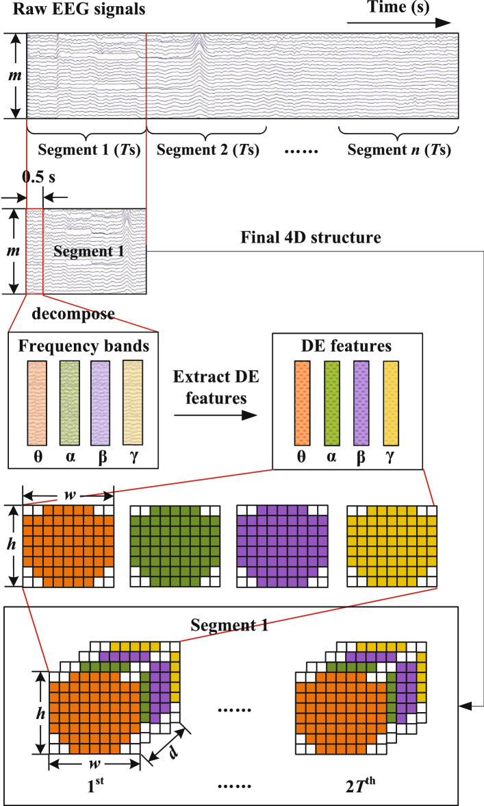
To integrate the frequency, spatial and temporal features of EEG signals simultaneously, we build a 4D feature structure including these three kinds of information as depicted in Fig. 2. Firstly, as previous works did (Yang et al. 2018a, b), to increase the amount of training data, we divide original EEG trials into Ts long segments without overlapping and assign every segment with the label of the original trial. Then, for each segment, we decompose it with a Butterworth filter into four frequency bands including , , and . Secondly, we extract differential entropy (DE) features from each frequency band with 0.5 s window, which has been proved to be the most stable feature for emotion recognition (Zheng et al. 2017; Duan et al. 2013). Thirdly, we organize the DE feature of each frequency band as a 2D map and stack them. Thus, every segment can be represented as a 4D structure , , where N is the number of total samples, h and w are the height and width of 2D map respectively, d represents the number of frequency bands and 2T denotes twice of the segment length. More details are described as follows.
Fig. 2.
The generation of 4D inputs
DE feature is used to measure the complexity of EEG signals, which is defined as
| 1 |
where Z is a random variable, f(z) is the probability density function of Z. Following previous studies (Zheng et al. 2017), the DE feature for Gaussian distribution is calculated as below
| 2 |
where Z follows the Gaussian distribution , e and are the Euler’s constant and the standard deviation of a time series, respectively.
Suppose an original EEG segment is represented as , where m and r denotes the number of electrodes and the sample rate of raw EEG signals, respectively. For each EEG segment, we calculate DE features for every frequency band with 0.5 s window and normalize each DE vector with Z-score normalization. Thus, the original EEG segment is transformed into the DE segment , where d denotes the number of frequency bands and we set it as 4 in this paper.
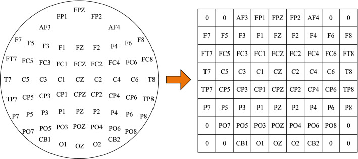
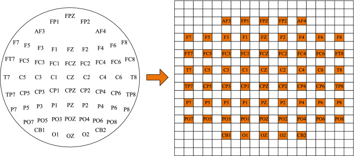
To keep the spatial structure information of the electrode location, we further transform the m-dimension DE vector into a compact 2D map according to the location of electrodes. For example, the 2D map of 62 channels is shown in Fig. 3, where zero denotes that the signals of the channels are unused. Then, we stack the 2D map of different bands into a 3D array, which is expected to combine complementary information of them. Therefore, the DE segment is converted into final segment representation , where h and w are the height and width of the compact 2D map, respectively. In this paper, we set and .
Fig. 3.
The compact 2D map of 62 channels
CRNN modeling
Frequency and spatial feature learning
For a sample (a 4D structure), we extract frequency and spatial information through CNN from each temporal slice of it. Different from traditional CNNs whose convolutional layer is usually followed by a pooling layer, we only add a pooling layer after the last convolutional layer. The pooling operation is used to reduce the parameter amount at the expense of information loss. However, the 2D map size of sample is really small that it had better preserve all information rather than merge information to reduce the number of parameters. Therefore, we only use one pooling layer after the last convolutional layer.
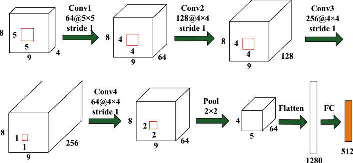
Our CNN module is similar to CNN structure in Yang et al. (2018a), while the difference is that we add a max-pooling layer after the last convolutional layer, and the reason is described above. As depicted in Fig. 4, it contains four convolutional layers, one max-pooling layer and one fully-connected layer. Specifically, the first convolutional layer (Conv1) has 64 feature maps with filter size of . The next two convolutional layers (Conv2, Conv3) respectively have 128 and 256 feature maps with filter size of . The fourth convolutional layer (Conv4) includes 64 feature maps with filter size of , which is used to fuse feature maps of the previous convolutional layer. For all convolutional layers, zero-padding and rectified linear units (ReLU) activation function are applied. After convolutional operations, a max-pooling layer (Pool) with size of and a stride of 2 is applied to ease overfitting and enhance the robustness of the network. Finally, outputs of the Pool layer are flattened and fed to a fully-connected layer (FC) with 512 units. The final output is the frequency and spatial representation of original EEG segments.
Fig. 4.
The structure of CNN module for frequency and spatial feature learning
Temporal feature learning
Since EEG signals contain dynamic content, the variations between temporal slices in the 4D structure may hid additional information which could be useful for making more accurate emotion classification. Thus, we utilize a RNN with LSTM cells to extract temporal information from CNN outputs.
Given a CNN output sequence , where and . We use a LSTM layers with 128 memory cells to excavate temporal dependency of inner segment, as shown in Fig. 5. The output of the LSTM layer can be calculated as follows
| 3 |
| 4 |
| 5 |
| 6 |
| 7 |
| 8 |
where is the logistic sigmoid function, and i, f, o and c are the input gate, forget gate, output gate and cell activation vectors. The W terms are weight matrices (e.g. is the hidden-input weight matrix), the b terms are bias vectors (e.g. is the input bias vector) respectively.
Fig. 5.
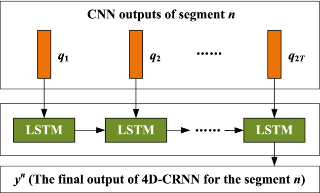
The structure of LSTM module for temporal feature learning
The final high-level representation of the EEG segment is the output of the last LSTM node, . It integrates the frequency, spatial and temporal cues of a Ts EEG segment.
Classifier
Based on the final feature representation , we predict the label of the original EEG segment by linear transform approach, which can be computed as
| 9 |
where A is the transform matrix, b is the bias and C is the number of emotion category. Then, the output is fed into a softmax classifier for emotion recognition, which can be formulated as
| 10 |
where represents the probability of the EEG segment belong to the class c.
Experiment
In this section, two public evaluation datasets are introduced. Then, the experiment setting of our method are described. Finally, the results on these datasets are reported and discussed.
Datasets
SEED dataset
The SEED dataset (Zheng and Lu 2015) carefully selects the emotional clips and healthy subjects, making sure that clips could elicit subjects’ corresponding emotion. There are 15 emotional clips selected from films. Each clip is about 4 min long and only contains one kind of emotion. These emotional clips can be divided into 3 categories of emotions (positive, neutral, and negative), and every 5 clips corresponds to one kind of emotion. 15 healthy subjects take part in the EEG signals collection experiment. Before each clip, subjects were provided a 15 s hint about the emotion category of the clip. After each clip, they were asked to record their self-assessment about the clip immediately. While they were watching the clips, EEG signals of them were recorded by 62-channels’ ESI NeuroScan system, whose electrodes are located according to the 10–20 system. After the experiments, according to the response of the subjects, only the trials when the target emotions were elicited were chosen for further analysis. Every subject conducts the above experiment three times, which means there are 3 sessions for each subject. We mixed all 3 sessions of each subject. If EEG signals were split into 2 s () without overlapping, we would obtain 5076 samples per subject. The EEG signals seriously contaminated by electromyography (EMG) and Electrooculography (EOG) had been already removed manually before the publication of the dataset. The data was downsampled to 200 Hz. A bandpass filter between 4 and 50 Hz was applied to EEG signals to filter the noise.
DEAP dataset
The DEAP dataset (Koelstra et al. 2012) uses music video clips as the visual stimuli to elicit different emotions. It contains 40 video clips, which chosen by using a web-based subjective emotion assessment interface. For each clip, it was segmented into 1 min which contained maximum emotional content. Thus, the final stimuli are 40 1-min video clips. The emotion category of each clip is labeled by the rated levels (1–9) of arousal and valence. We choose 5 as the threshold to divide the labels into two binary classification problems, which is the same as previous works did (Yang et al. 2018a, b). There are 32 subjects invited to watch these clips. Their EEG signals were collected by 32-channels’ Biosemi ActiveTwo device according to the international 10–20 system. During the experiments, subjects performed a self-assessment of their levels of arousal, valence at the end of each trial, which used to judge whether the corresponding emotion was elicited correctly. EMG and EOG signals had been removed before the publication of the dataset. EEG signals were downsampled to 128 Hz. They were passed to a bandpass filter between 4 and 45 Hz to filter the noise.
For each trial (a trial means a subject watches one video clip), it contains 63 s EEG signals. The first 3 s of signals are pre-trial baseline signals in a relaxed state. The rest 60 s of EEG recordings are emotional signals. Since Yang et al. (2018a) and Yang et al. (2018b) have demonstrated that the baseline signals are useful for emotion recognition, we process the signals as they did. We first divide the baseline signals into 6 segments with 0.5 s and extract DE features from four frequency bands (, , , ) of each segment. Then, the baseline DE features are calculated by averaging DE features of these 6 segments for each frequency band. Finally, the difference between baseline DE features and emotional DE features is used by our method. Therefore, for each subject, it has 40 60 s EEG signals. If we take one sample per 2 s () without overlapping, 1200 samples will be gained for each subject.
Experimental setup
4D-CRNN is trained with a batch size of 128 and Adam with a learning rate of 0.001. The maximum number of epochs is set as 100. Note that all these training hyper-parameters were optimized on the test set. The model is implemented by Keras,1 which is extended from Google Tensorflow,2 and trained on a NVIDIA GTX TITAN X GPU. Codes are available at https://github.com/aug08/4D-CRNN.
We evaluate performances of all methods for EEG emotion recognition with a similar protocol used in Li et al. (2018) and Yang et al. (2018a). Specifically, we applied fivefold cross-validation on each subject, the average classification accuracy (ACC) and standard deviation (STD) of them represent the individual performance for the subject. The average ACC and STD of all subjects denote the final performance of the method.
Results
The proposed 4D-CRNN network takes 4D segments with size as inputs. In this paper, we set because results of previous studies have shown that the combination of all bands can complement each other and contribute to better results than individual bands (Zheng and Lu 2015; Yang et al. 2018a). Parameters h, w and T affect the amount of spatial and temporal cues of EEG signals that our model could perceive. Therefore, we investigate the effect of EEG segment length (T) and the effect of 2D map (h and w) on the recognition accuracy. Then, we evaluate the overall performance of our model. Finally, we make a comparison with other traditional structures.
The effect of EEG segment length
Since the length of EEG segment determines the emotion information it contains, we investigate the segment length T ranges in [1, 1.5, 2, 2.5, 3, 3.5, 4]. Besides, we set h, w and d as 8, 9 and 4, respectively. Table 1 shows the performances (average ACC and STD of all subjects) of different T using 4D-CRNN on SEED and DEAP datasets.
Table 1.
Performances (average ACC ± STD %) of segment length T using 4D-CRNN on SEED and DEAP
| T (s) | SEED | DEAP-valence | DEAP-arousal |
|---|---|---|---|
| 1.0 | 93.99 ± 2.57 | 93.52 ± 3.26 | 93.78 ± 4.19 |
| 1.5 | 94.59 ± 2.37 | 93.84 ± 3.36 | 94.19 ± 4.02 |
| 2.0 | 94.74 ± 2.32 | 94.22 ± 2.61 | 94.58 ± 3.69 |
| 2.5 | 94.38 ± 2.51 | 93.97 ± 3.06 | 94.36 ± 3.76 |
| 3.0 | 94.02 ± 2.45 | 94.20 ± 2.78 | 94.46 ± 3.81 |
| 3.5 | 93.24 ± 3.57 | 93.95 ± 2.91 | 94.42 ± 4.00 |
| 4.0 | 93.84 ± 2.67 | 94.11 ± 2.77 | 94.42 ± 3.72 |
From the results, we can draw two conclusions. First, setting seems the optimal segment length for EEG-based emotion recognition, since it achieves the best performance both on SEED and DEAP. On SEED, when setting , the corresponding average ACC and STD for discrete emotion classification are 94.74 ± 2.32%. On DEAP, the corresponding average ACCs and STDs are 94.22 ± 2.16% and 94.58 ± 3.69% for valence and arousal classification tasks, respectively. Second, the difference between the accuracies of different segment length is fairly small. On SEED, the biggest gap is 1.35% when comparing and . On DEAP, the largest gaps are 0.7% and 0.8% for valence and arousal classification, respectively. This indicates that our method can extract inherent temporal information from EEG and not is affected by the length of the segment. In the remaining paper, is chosen as the segment length.
The effect of 2D map
In general, there are two kinds of 2D maps that electrodes can be transformed, one is a compact map as we did, another is a sparse map used in Li et al. (2018). For instance, 62 channels can be transformed into a sparse 2D map as displayed in Fig. 6. In this part, we examine the effects of them with 4D-CRNN. Our compact map is shaped as , while the sparse map is . We calculate the average ACC, STD and time cost of all subjects to indicate the performance of each map.
Fig. 6.
The sparse 2D map of 62 channels
Results on the SEED dataset are presented in Table 2, which can be found that the accuracy of our compact map is closed to the sparse map. The accuracy of the compact map is 94.74%, which is only 0.29% less than the sparse map. While for the time cost of them, the compact map only spends 811 s for every subject in fivefold cross-validation, which is almost one-third of the time cost of the sparse map. On the DEAP dataset, as shown in Table 3, the performance of our compact map is better than the sparse map both from accuracy and training time cost aspects. For the valence classification, the average accuracy of the compact map is 94.22%, which exceeds the accuracy of the sparse map by 1.06%. Besides, the average time cost of the compact map is 59 s, while the time spending by the sparse map is 137 s, which is more than twice of compact map. For arousal classification, we can obtain similar conclusions. The reason for obtaining similar results maybe because that the sparse map adding zeros between adjacent electrodes does not increase any useful information. The less time cost of compact map is likely due to the smaller size of it, which involves less convolutional filters to be calculated.
Table 2.
The comparison between two kinds of 2D maps on SEED
| 2D map | Map shape | ACC ± STD (%) | Time cost (s) |
|---|---|---|---|
| Compact map (ours) | 8 × 9 | 94.74 ± 2.32 | 811 |
| Sparse map (Li et al. 2018) | 19 × 19 | 95.03 ± 2.23 | 2274 |
Table 3.
The comparison between two kinds of 2D maps on DEAP
| 2D map | Map shape | Valence | Arousal | ||
|---|---|---|---|---|---|
| ACC ± STD (%) | Time cost (s) | ACC ± STD (%) | Time cost (s) | ||
| Compact map (ours) | 8 × 9 | 94.22 ± 2.61 | 295 | 94.58 ± 3.69 | 300 |
| Sparse map (Li et al. 2018) | 19 × 19 | 93.16 ± 3.14 | 685 | 93.20 ± 4.18 | 675 |
Results on both datasets have persuaded us that comparing with the sparse map, the compact map is the better choice to categorize emotions. Therefore, we chose the compact map, where and , in the remaining paper.
Overall performance
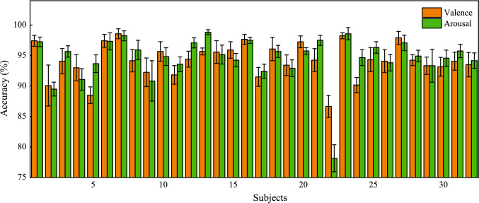
In this part, we display the overall performances of 4D-CRNN on SEED and DEAP datasets with the optimal parameters according to the above analysis, where , and . From Fig. 7, we can find that 4D-CRNN is stably effective on the SEED dataset. Accuracies of all subjects are surpassed 90% and the average accuracy of them achieves 94.74% with STD 2.32%. Among 15 subjects, there are 9 of them (#2, #4, #5, #6, #8, #9, #10, #13 and #14) outperform than the average accuracy. Results of 4D-CRNN model on DEAP are shown in Fig. 8. For valence classification, the mean accuracy and STD of all 32 subjects are 94.22% and 2.61% respectively, and there are 30 subjects (except #5 and #22) higher than 90%. For arousal classification, the mean accuracy is 94.58% and the STD is 3.69%. There are only 2 subjects (#2 and #22) lower than 90% in terms of accuracy. It is worth noting that the valence and arousal accuracies of subject #22 are 86.67% and 78.16%, respectively, which is lower than others. This might because the subject lacked concentration during the experiments or did not well report the degree of subjective feeling after experiments.
Fig. 7.
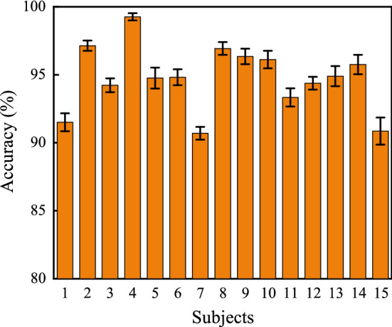
Overall performance of the 4D-CRNN model on SEED
Fig. 8.
Overall performance of the 4D-CRNN model on DEAP
Method comparison
To show effective performances of our proposed method, we conduct a comparison with several commonly used methods, which are listed below:
HCNN (Li et al. 2018) It used the hierarchical CNN architecture to classify emotions. The first convolutional layer had 6 feature maps with filter size of , followed by a max-pooling layer with size of . The second convolutional layer had 16 feature maps with filter size of , followed by a max-pooling layer with size of . After them, there was a fully-connected layer with 144 nodes. It took 2D DE maps () as inputs, and the DE features only extracted from frequency band. It only considered the spatial information of EEG signals.
CCNN (Yang et al. 2018a) It built a continuous CNN model which constructed by four convolutional layers and one fully-connected layer. The size of feature maps and filters of the four convolutional layers were {64, 128, 256, 64} and {, , , }, respectively. The fully-connected layer had 1024 nodes. It took 3D DE structures () as inputs, where DE features extracted from four frequency bands (, , , ). It excavated frequency and spatial cues from EEG signals.
EmotionNet (Wang et al. 2018) It utilized 3D convolution kernels to extract spatial and temporal features simultaneously from raw EEG signals. In the first two layers, the size of 3D kernels was set as to extract spatio-temporal information. In the third layer, the 3D kernel size was set as to fuse spatial information only. In the fourth and fifth layers, the kernel was to extract temporal features only. It took 3D structure () of raw EEG signals as input, where r denoted the sample rate of EEG signals. This model contained spatio-temporal information of EEG signals.
PCRNN (Yang et al. 2018b) It utilized CNN to extract spatial features from each 2D map, and used LSTM to extract temporal features from the EEG vector sequence. After that, the spatial features and temporal features were concatenated to make emotion classification. It took 3D structure () of raw EEG signals as input. This method parallelly integrated spatial and temporal information from raw EEG signals to classify emotions.
CNN (Ours) It was the CNN module of our method which contained four convolutional layers, a max-pooling layer and a fully-connected layer. The structure details of it is shown in Fig. 4. It took 2D map () or 3D structure () of DE features as input. It extracted frequency and spatial information from EEG signals.
CRNN (Ours) It was the CRNN module of our method, which combined by CNN module shown in Fig. 4 and a LSTM layer shown in Fig. 5. It used 3D structure () as input. It extracted spatial and temporal information from raw EEG signals.
For the first four methods, we reproduce these methods according to the structure parameters presented in the original papers. We apply these methods on SEED and DEAP datasets with fivefold cross-validation. The length of each sample is set as 2 s, then we get 5070 samples for each subject in the SEED dataset, 1200 samples for each subject in the DEAP dataset. The 2D map is compact. Table 4 shows the average ACC and STD of each method. On the SEED dataset, the accuracy of 4D-CRNN is 94.74%, which exceeds the accuracy of HCNN by 6.14%. On the DEAP dataset, the valence classification accuracy of 4D-CRNN is 94.22%, which beats EmotionNet, CCNN and PCRNN by a margin of 20.82%, 4.42% and 3.96%, respectively. Arousal classification accuracy of 4D-CRNN is 94.58%, which outperforms the other three methods by 20.32%, 4.08 and 3.60% respectively.
Table 4.
The performances (average ACC ± STD (%)) of the compared methods.
| Nos. | Method | Input shape | Information | SEED | DEAP-valence | DEAP-arousal |
|---|---|---|---|---|---|---|
| 1 | HCNN (Li et al. 2018) | Frequency + spatial | 88.60 ± 2.60** | – | – | |
| 2 | CCNN (Yang et al. 2018a) | Frequency + spatial | – | 89.80 ± 2.76** | 90.50 ± 2.98** | |
| 3 | EmotionNet (Wang et al. 2018) | Spatial + temporal | – | 73.40 ± 3.13** | 74.26 ± 3.08** | |
| 4 | PCRNN (Yang et al. 2018b) | Spatial + temporal | – | 90.26 ± 2.88** | 90.98 ± 3.09** | |
| 5 | CNN (ours) | Frequency + spatial | 90.88 ± 2.43 | 88.76 ± 2.32 | 88.92 ± 2.15 | |
| 6 | CNN (ours) | Frequency + spatial | 92.16 ± 3.52 | 91.03 ± 2.49 | 92.16 ± 2.78 | |
| 7 | CRNN (ours) | Spatial + temporal | 92.88 ± 3.12 | 91.98 ± 3.60 | 92.46 ± 3.35 | |
| 8 | 4D-CRNN (ours) | Frequency + spatial + temporal | 94.74 ± 2.32 | 94.22 ± 2.61 | 94.58 ± 3.69 |
The symbol “**” indicates statistic significance (paired t test, ) of performance improvement of the proposed method (4D-CRNN) in comparison with other methods
To illustrate the statistical significance between our proposed 4D-CRNN method and the other methods (HCNN, CCNN, EmotionNet and PCRNN), we perform the paired t-test on their classification results. The hypothesis is that “the classification performance of 4D-CRNN is greater than that of the other methods”. Each test is run on the two sequences of the classification results obtained by 4D-CRNN and the given method. The statistical test results are represented by the symbol “**”, which means that the hypothesis is correct with probability 0.99. For example, on the DEAP dataset, the average valence classification accuracy of 4D-CRNN over fivefold is 94.22 ± 2.61% and that of PCRNN is 90.26 ± 2.88%. The appended “**” means the hypothesis of 4D-CRNN is superior to PCRNN is true based on the statistical test. In summary, from Table 4, we conclude that 4D-CRNN achieves better performance than the other compared methods on both datasets.
To verify the effectiveness of our CNN module on frequency and spatial feature extracting, we compare it with HCNN and CCNN. As shown experiments #1 and #5 in Table 4, we feed the same inputs (, which is a 2D map of DE features extracted from frequency band) into HCNN and CNN (Ours), respectively. It can be found that our CNN module yields an increase of 2.28%. When compared CCNN with CNN (Ours), we feed the same inputs (, which is a 3D structure of DE features extracted from , , and frequency band) into them. The classification results can be found in Table 4 experiments #2 and #6. It can be observed that our CNN provides an improvement in accuracy with 1.23% and 1.66% for valence and arousal classification, respectively. Thus, we can conclude that our CNN module outperforms HCNN and CCNN in frequency and spatial feature learning. Reasons will be discussed in “Discussion” section.
To investigate the effectiveness of our CRNN module on spatial and temporal information learning, we compare it with EmotionNet and PCRNN models. We feed the same inputs (, which is a 3D structure of raw EEG signals) into these three models, respectively. The results are shown in Table 4 experiments #3, #4 and #7. The EmotionNet gets the worst performance, which lower than CRNN (Ours) on valence and arousal classification by 18.58% and 18.2%, respectively. When compared with PCRNN, CRNN (Ours) displays better performance, which exceeds PCRNN by 1.72% and 1.48% for valence and arousal classification, respectively. Therefore, we conclude that our CRNN can extract spatial and temporal information from EEG effectively. Reasons that CRNN outperforms EmotionNet and PCRNN will be displayed latter.
As shown in Table 4 experiments #6, #7 and #8. CNN only can extract frequency and spatial information from EEG signals. CRNN not only can extract spatial and temporal such as experiment #7, but also can learn frequency, spatial and temporal information at the same time, such as experiment #8. It mainly depends on the input it is fed. To verify the importance of simultaneously considering frequency, spatial and temporal information of EEG signals for emotion recognition, we compare 4D-CRNN (Ours) with CNN (Ours) and CRNN (Ours). From the results, 4D-CRNN gets the best results both on SEED and DEAP datasets. 4D-CRNN outperforms CNN by 2.58% on SEED, 3.19% and 2.42% on valence and arousal classification on DEAP, respectively. 4D-CRNN exceeds CRNN by 1.86% on SEED, 2.33% and 2.12% on valence and arousal tasks, respectively. We can conclude that simultaneously taking frequency, spatial and temporal information into account is benefit for emotion recognition. The superiority of the proposed 4D feature structure will be discussed latter.
Discussion
The above-mentioned comparison analysis shows that our 4D-CRNN architecture performs best than other methods. Several noteworthy points will be discussed in this section.
First, slightly deeper convolutional layers and max-pooling are benefit for CNN to extract and preserve more information. From Table 4 experiments #1, #2 and #5, we can find that the results of CNN (Ours) are better than HCNN and CCNN. Compared CNN (Ours) with HCNN, it yields a large increase of 2.28%. This may be because our CNN is deeper, which containing 4 convolutional layers and each convolutional layer has {64, 128, 256, 64} feature maps, respectively. However, HCNN only contains 2 convolutional layers and they respectively contain {6, 16} feature maps. Thus, our CNN can extract more emotion related cues than HCNN. As for CCNN, our CNN provides an improvement in accuracy with 1.23% and 1.66% for valence and arousal classification, respectively. This may be due to that the max-pooling contributes to preserving useful information.
Second, the deeper fusion of CNN and LSTM is better for extracting spatial and temporal information than parallel concatenating of CNN and LSTM. From Table 4, CRNN (Ours) displays better performance than PCRNN for EEG based emotion recognition. Although they both contain CNN and LSTM modules, the combination ways are different. CRNN firstly extracts spatial features by CNN from each 2D map of 3D EEG structure. Then utilizes LSTM to extract temporal information from CNN outputs which contain high-level spatial features. Finally, the outputs of the LSTM module are used to make the classification. However, PCRNN extracts spatial features by CNN from 2D EEG maps, while extracting temporal features by LSTM from EEG vectors, then concatenate the outputs of CNN and LSTM to make the classification. The results of CRNN exceed that of PCRNN maybe because it takes the spatial topology of electrodes into consideration when extracting temporal information of EEG signals, which makes these two kinds of information complement each other better. EmotionNet gets the worst performance among them, which maybe because LSTM layers are more suitable for extracting temporal information from EEG signals than 3D kernels.
Third, the 4D feature structure integrating frequency, spatial and temporal information of EEG performs better than 2D and 3D structures which without containing these three kinds of information simultaneously. The accuracy of 4D-CRNN is better than other compared methods displayed in Table 4, which might be partly attributed to the organization of the input feature. 4D-CRNN uses 4D structures as inputs, while CNN and CRNN take 2D or 3D structures as inputs. Firstly, the 4D feature structure contains frequency information extracted from four frequency bands (, , and ), which already have been proved to be associated with emotion (Zheng and Lu 2015; Yang et al. 2018a). Besides, it maintains the spatial topology of electrodes by the 2D map, which preserving spatial information of multichannel. What is more, it comprises temporal information since it contains contiguous DE features with several seconds, which can capture the dynamic content of emotion without varying with time. However, 2D and 3D feature structures only involve two of these three kinds of information. Therefore, 4D feature structure contains more cues of emotion than other structures and performs better than them.
Conclusion
We presented a segment-level EEG-based emotion classification method capable of aggregating frequency, spatial and temporal information of EEG signals into account. The proposed method achieves state-of-the-art performance both on SEED and DEAP datasets. The vital procedures lie in two parts: first, we build the EEG signals into 4D feature structures, which explicitly organize frequency, spatial and temporal cues of EEG. Second, we introduce the CRNN model which is deeply fused by CNN and LSTM. CNN deals with the frequency and spatial information and LSTM extracts temporal dependencies from CNN outputs. We investigate the importance of simultaneously extracting frequency, spatial and temporal information from EEG by comparing it with four competitive studies. The performance is greatly improved due to the involvement of these three kinds of cues in EEG-based emotion classification.
Acknowledgements
This work is supported by the National Key R&D Program of China (2017YFE0118200 and 2017YFE0116800), NSFC (61633010), key Research and Development Project of Zhejiang Province (2020C04009), Fundamental Research Funds for the Provincial Universities of Zhejiang (GK209907299001-008). The authors also thank the National International Joint Research Center for Brain-Machine Collaborative Intelligence (2017B01020), Key Laboratory of Brain Machine Collaborative Intelligence of Zhejiang Province (2020E10010).
Footnotes
Publisher's Note
Springer Nature remains neutral with regard to jurisdictional claims in published maps and institutional affiliations.
References
- Akin M. Comparison of wavelet transform and FFT methods in the analysis of EEG signals. J Med Syst. 2002;26(3):241–247. doi: 10.1023/A:1015075101937. [DOI] [PubMed] [Google Scholar]
- Alarcão SM, Fonseca MJ. Emotions recognition using EEG signals: a survey. IEEE Trans Affect Comput. 2017;10(3):374–393. doi: 10.1109/TAFFC.2017.2714671. [DOI] [Google Scholar]
- Ansari-Asl K, Chanel G, Pun T (2007) A channel selection method for EEG classification in emotion assessment based on synchronization likelihood. In: European signal processing conference (EUSIPCO). IEEE, New York, pp 1241–1245
- Aricò P, Borghini G, Flumeri GD, Sciaraffa N, Babiloni F. Passive BCI beyond the lab: current trends and future directions. Physiol Meas. 2018;39(8):57. doi: 10.1088/1361-6579/aad57e. [DOI] [PubMed] [Google Scholar]
- Aricò P, Reynal M, Di Flumeri G, et al. How neurophysiological measures can be used to enhance the evaluation of remote tower solutions. Front Hum Neurosci. 2019;13:303. doi: 10.3389/fnhum.2019.00303. [DOI] [PMC free article] [PubMed] [Google Scholar]
- Aricò P, Sciaraffa N, Babiloni F. Brain–computer interfaces: toward a daily life employment. Brain Sci. 2020 doi: 10.3390/brainsci10030157. [DOI] [PMC free article] [PubMed] [Google Scholar]
- Bamdad M, Zarshenas H, Auais MA. Application of BCI systems in neurorehabilitation: a scoping review. Disab Rehab Assist Technol. 2015;10(5):355–364. doi: 10.3109/17483107.2014.961569. [DOI] [PubMed] [Google Scholar]
- Blankertz B, Acqualagna L, Dähne S, Haufe S, Schultze-Kraft M, Sturm I, Ušćumlic M, Wenzel MA, Curio G, Müller KR. The Berlin brain–computer interface: progress beyond communication and control. Front Neurosci. 2016;10:530. doi: 10.3389/fnins.2016.00530. [DOI] [PMC free article] [PubMed] [Google Scholar]
- Cartocci G, Maglione AG, Vecchiato G, Flumeri GD, Colosimo A, Scorpecci A, Marsella R, Giannantonio S, Malerba P, Borghini G, Aricò P, Babiloni F (2015) Mental workload estimations in unilateral deafened children. In: 2015 37th annual international conference of the IEEE engineering in medicine and biology society (EMBC). IEEE, New York, pp 1654–1657 [DOI] [PubMed]
- Chen X, Pan Z, Wang P, Zhang L, Yuan J. EEG oscillations reflect task effects for the change detection in vocal emotion. Cogn Neurodyn. 2015;9(3):351–358. doi: 10.1007/s11571-014-9326-9. [DOI] [PMC free article] [PubMed] [Google Scholar]
- Cowie R, Douglas-Cowie E, Tsapatsoulis N, Votsis G, Kollias S, Fellenz W, Taylor JG. Emotion recognition in human–computer interaction. IEEE Signal Process Mag. 2001;18(1):32–80. doi: 10.1109/79.911197. [DOI] [Google Scholar]
- Duan RN, Zhu JY, Lu BL (2013) Differential entropy feature for EEG-based emotion classification. In: 2013 6th international IEEE/EMBS conference on neural engineering (NER). IEEE, New York, pp 81–84
- Figueiredo GR, Ripka WL, Romaneli EFR, Ulbricht L (2019) Attentional bias for emotional faces in depressed and non-depressed individuals: an eye-tracking study. In: 2019 41st annual international conference of the IEEE engineering in medicine and biology society (EMBC). IEEE, New York, pp 5419–5422 [DOI] [PubMed]
- Fiorini L, Mancioppi G, Semeraro F, Fujita H, Cavallo F. Unsupervised emotional state classification through physiological parameters for social robotics applications. Knowl Based Syst. 2020 doi: 10.1016/j.knosys.2019.105217. [DOI] [Google Scholar]
- Frantzidis CA, Bratsas C, Papadelis CL, Konstantinidis E, Pappas C, Bamidis PD. Toward emotion aware computing: an integrated approach using multichannel neurophysiological recordings and affective visual stimuli. IEEE Trans Inf Technol Biomed. 2010;14(3):589–597. doi: 10.1109/TITB.2010.2041553. [DOI] [PubMed] [Google Scholar]
- Garcia-Molina G, Tsoneva T, Nijholt A. Emotional brain–computer interfaces. Int J Auton Adap Commun Syst. 2013;6(1):9–25. doi: 10.1504/IJAACS.2013.050687. [DOI] [Google Scholar]
- Goshvarpour A, Goshvarpour A. EEG spectral powers and source localization in depressing, sad, and fun music videos focusing on gender differences. Cogn Neurodyn. 2019;13(2):161–173. doi: 10.1007/s11571-018-9516-y. [DOI] [PMC free article] [PubMed] [Google Scholar]
- He K, Zhang X, Ren S, Sun J (2016) Deep residual learning for image recognition. In: Proceedings of the IEEE conference on computer vision and pattern recognition (CVPR), pp 770–778
- Hochreiter S, Schmidhuber J. Long short-term memory. Neural Comput. 1997;9(8):1735–1780. doi: 10.1162/neco.1997.9.8.1735. [DOI] [PubMed] [Google Scholar]
- Hsu YL, Wang JS, Chiang WC, Hung CH. Automatic ECG-based emotion recognition in music listening. IEEE Trans Affect Comput. 2017;11(1):85–99. doi: 10.1109/TAFFC.2017.2781732. [DOI] [Google Scholar]
- Koelstra S, Muhl C, Soleymani M, Lee JS, Yazdani A, Ebrahimi T, Pun T, Nijholt A, Patras I. Deap: a dataset for emotion analysis using physiological signals. IEEE Trans Affect Comput. 2012;3(1):18–31. doi: 10.1109/T-AFFC.2011.15. [DOI] [Google Scholar]
- Kong WZ, Zhou ZP, Jiang B, Babiloni F, Borghini G. Assessment of driving fatigue based on intra/inter-region phase synchronization. Neurocomputing. 2017;219:474–482. doi: 10.1016/j.neucom.2016.09.057. [DOI] [Google Scholar]
- Krizhevsky A, Sutskever I, Hinton GE (2012) Imagenet classification with deep convolutional neural networks. In: Advances in neural information processing systems (NIPS), pp 1097–1105
- Kroupi E, Yazdani A, Ebrahimi T (2011) EEG correlates of different emotional states elicited during watching music videos. In: International conference on affective computing and intelligent interaction. Springer, Berlin, pp 457–466
- Li M, Lu BL (2009) Emotion classification based on gamma-band EEG. In: 2009 annual international conference of the IEEE engineering in medicine and biology society. IEEE, New York, pp 1223–1226 [DOI] [PubMed]
- Li JP, Zhang ZX, He HG. Hierarchical convolutional neural networks for EEG-based emotion recognition. Cogn Comput. 2018;10(2):368–380. doi: 10.1007/s12559-017-9533-x. [DOI] [Google Scholar]
- Ma JX, Tang H, Zheng WL, Lu BL (2019) Emotion recognition using multimodal residual LSTM network. In: Proceedings of the 27th ACM international conference on multimedia (MM), pp 176–183
- Murugappan M, Rizon M, Nagarajan R, Yaacob S. Inferring of human emotional states using multichannel EEG. Eur J Sci Res. 2010;48(2):281–299. [Google Scholar]
- Mühl C, Allison B, Nijholt A, Chanel G. A survey of affective brain computer interfaces: principles, state-of-the-art, and challenges. Brain Comput Interfaces. 2014;1(2):66–84. doi: 10.1080/2326263X.2014.912881. [DOI] [Google Scholar]
- Pfurtscheller G, Allison BZ, Brunner C, Bauernfeind G, Solis-Escalante T, Scherer R, Zander TO, Mueller-Putz G, Neuper C, Birbaumer N. The hybrid BCI. Front Hum Neurosci. 2010;4:42. doi: 10.3389/fnpro.2010.00003. [DOI] [PMC free article] [PubMed] [Google Scholar]
- Reuderink B, Mühl C, Poel M. Valence, arousal and dominance in the EEG during game play. Int J Auton Adapt Commun Syst. 2013;6(1):45–62. doi: 10.1504/IJAACS.2013.050691. [DOI] [Google Scholar]
- Rozgić V, Vitaladevuni SN, Prasad R. Robust EEG emotion classification using segment level decision fusion. In: 2013 IEEE international conference on acoustics, speech and signal processing (ICASSP). IEEE, New York, pp 1286–1290
- Song TF, Zheng WM, Song P, Cui Z. EEG emotion recognition using dynamical graph convolutional neural networks. IEEE Trans Affect Comput. 2018 doi: 10.1109/TAFFC.2018.2817622. [DOI] [Google Scholar]
- Vansteensel MJ, Jarosiewicz B. Brain–computer interfaces for communication. Handb Clin Neurol. 2020;168:67–85. doi: 10.1016/B978-0-444-63934-9.00007-X. [DOI] [PubMed] [Google Scholar]
- Wang Y, Huang ZY, McCane B, Neo P (2018) EmotioNet: a 3-D convolutional neural network for EEG-based emotion recognition. In: 2018 international joint conference on neural networks (IJCNN). 10.1109/IJCNN.2018.8489715
- Yan JJ, Zheng WM, Xu QY, Lu GM, Li HB, Wang B. Sparse kernel reduced-rank regression for bimodal emotion recognition from facial expression and speech. IEEE Trans Multimed. 2016;18(7):1319–1329. doi: 10.1109/TMM.2016.2557721. [DOI] [Google Scholar]
- Yang YL, Wu QF, Fu YZ, Chen XW (2018a) Continuous convolutional neural network with 3D input for EEG-based emotion recognition. In: International conference on neural information processing (ICONIP). Springer, Berlin, pp 433–443
- Yang YL, Wu QF, Qiu M, Wang TD, Chen XW (2018b) Emotion recognition from multi-channel EEG through parallel convolutional recurrent neural network. In: 2018 international joint conference on neural networks (IJCNN). 10.1109/IJCNN.2018.8489331
- Zeng H, Yang C, Dai GJ, Qin FW, Zhang JH, Kong WZ. EEG classification of driver mental states by deep learning. Cogn Neurodyn. 2018;12(6):597–606. doi: 10.1007/s11571-018-9496-y. [DOI] [PMC free article] [PubMed] [Google Scholar]
- Zeng H, Wu ZH, Zhang JM, Yang C, Zhang H, Dai GJ, Kong WZ. EEG emotion classification using an improved SincNet-based deep learning model. Brain Sci. 2019 doi: 10.3390/brainsci9110326. [DOI] [PMC free article] [PubMed] [Google Scholar]
- Zeng H, Yang C, Zhang H, Wu ZH, Zhang JM, Dai GJ, Babiloni F, Kong WZ. A lightGBM-based EEG analysis method for driver mental states classification. Comput Intell Neurosci. 2019 doi: 10.1155/2019/3761203. [DOI] [PMC free article] [PubMed] [Google Scholar]
- Zhang T, Zheng WM, Cui Z, Zong Y. Spatio-temporal recurrent neural network for emotion recognition. IEEE Trans Cybern. 2018;49(3):839–847. doi: 10.1109/TCYB.2017.2788081. [DOI] [PubMed] [Google Scholar]
- Zhang ZX, Wu BW, Schuller B (2019) Attention-augmented end-to-end multi-task learning for emotion prediction from speech. In: IEEE international conference on acoustics, speech and signal processing (ICASSP). IEEE, New York, pp 6705–6709
- Zheng WL, Lu BL. Investigating critical frequency bands and channels for EEG-based emotion recognition with deep neural networks. IEEE Trans Auton Ment Dev. 2015;7(3):162–175. doi: 10.1109/TAMD.2015.2431497. [DOI] [Google Scholar]
- Zheng WL, Zhu JY, Lu BL. Identifying stable patterns over time for emotion recognition from EEG. IEEE Trans Affect Comput. 2017;10(3):417–429. doi: 10.1109/TAFFC.2017.2712143. [DOI] [Google Scholar]


