Highlights
-
•
A high-performance pneumonia detection system was proposed in this paper.
-
•
Transfer learning is used to obtain feature extractor.
-
•
A novel graph-based feature reconstruction method was proposed.
-
•
The proposed feature reconstruction is efficient yet transplantable to other scenarios.
Keywords: COVID-19, Chest X-ray images, Transfer learning, Graph, Feature reconstruction
Abstract
Pneumonia is a global disease that causes high children mortality. The situation has even been worsening by the outbreak of the new coronavirus named COVID-19, which has killed more than 983,907 so far. People infected by the virus would show symptoms like fever and coughing as well as pneumonia as the infection progresses. Timely detection is a public consensus achieved that would benefit possible treatments and therefore contain the spread of COVID-19. X-ray, an expedient imaging technique, has been widely used for the detection of pneumonia caused by COVID-19 and some other virus. To facilitate the process of diagnosis of pneumonia, we developed a deep learning framework for a binary classification task that classifies chest X-ray images into normal and pneumonia based on our proposed CGNet. In our CGNet, there are three components including feature extraction, graph-based feature reconstruction and classification. We first use the transfer learning technique to train the state-of-the-art convolutional neural networks (CNNs) for binary classification while the trained CNNs are used to produce features for the following two components. Then, by deploying graph-based feature reconstruction, we, therefore, combine features through the graph to reconstruct features. Finally, a shallow neural network named GNet, a one layer graph neural network, which takes the combined features as the input, classifies chest X-ray images into normal and pneumonia. Our model achieved the best accuracy at 0.9872, sensitivity at 1 and specificity at 0.9795 on a public pneumonia dataset that includes 5,856 chest X-ray images. To evaluate the performance of our proposed method on detection of pneumonia caused by COVID-19, we also tested the proposed method on a public COVID-19 CT dataset, where we achieved the highest performance at the accuracy of 0.99, specificity at 1 and sensitivity at 0.98, respectively.
1. Introduction
Pneumonia is a common yet serious lung disease caused by viruses and bacteria. Though it is treatable under most situations, timely detection still plays a key role in making diagnosis and treatment. Since the outbreak of COVID-19, Viral nucleic acid techniques(VNATs) and imaging techniques have been widely used to quickly diagnose pneumonia caused by COVID-19. It was reported that the sensitivity of VNATs was high (Behzadi, Ranjbar & Alavian, 2014), the false positive rate, however, is relatively high when compared to imaging-based detection methods (Fang et al. 2020). As pointed out by authors in Fang et al. (2020), a VNAT using real-time polymerase chain reaction (RT-PCR) achieved a sensitivity at 71% on a 51 cases dataset, however, Chest computed tomography (CT) showed sensitivity at 98%. Chest X-ray imaging has also been extensively deployed for the detection of pneumonia caused by COVID-19 (Adhikari, 2020; Islam, Wijewickrema, Collins & O'Leary, 2020; Rajpurkar et al., 2017). Compared to VNATs, Chest X-ray imaging is more accurate and convenient, which makes Chest X-ray to be the most popular technique for diagnosis of pneumonia (Chen et al., 2019). Also, compared to CT, X-ray is more popular because of the low cost and convenience of imaging. However, manual interpretation of the digitalized images, a time-consuming task, remains to be a challenging job for the radiologists due to the complexity and artificial factors. Therefore, automatic systems that can help radiologists with the understanding of images is demanding and would be greatly helpful to slow the spreading of COVID-19.
Deep learning (DL), a fast-developing branch of Machine Learning (ML), has shown great power over image classification and detection. Compared to classical ML methods, which heavily rely on manually crafted features, Deep Convolutional Neural Networks (CNNs), the most typical models of DL, have achieved eye-attracting success on considerable image-based tasks such as detection, classification and segmentation (He, Zhang, Ren & Sun, 2016; Ronneberger, Fischer & Brox, 2015; Zhao, Zheng, Xu & Wu, 2019). DL models, which are usually trained on millions of images, learn more abstract features than traditional ML models that focus on learning more straightforward but less representative features. Therefore, DL models have been showing huge advantages over traditional ML models on accuracy, flexibility and robustness. In some areas, DL models even outperformed the experts in the area by a large margin He Kaiming, Shaoqing and Jian (2016); He, Zhang, Ren and Sun (2015). Given the stated superiority, DL techniques have been embedded in many Computer-aided (CAD) systems. For DL systems, how to effectively embed useful information into the systems determines the final performance of the systems. There are considerable research works on information embedding (Li, Zhang, Qin, Zhang & Shao, 2019; Shen et al., 2021; Wen, Zhang, Zhang, Fei & Wang, 2020; Zhang et al., 2019, 2020; Zhang, Liu, Shen, Shen & Shao, 2018).
In this research, we proposed a new DL model named CGNet framework, which was featured by the proposed feature reconstruction method. Based on the proposed framework, a new high-performance pneumonia detection system was developed. In our proposed CGNet framework, there are three modules including feature extraction and graph-based feature reconstruction and classification. For the feature extraction, we transferred the state-of-the-art networks and trained with pneumonia datasets. High-level features, which are coarse features for further classification, can then be acquired through the trained networks. Based on the extracted features, we propose to integrate graph representation between individual images to improve the accuracy of the following classifier GNet, which has the same architecture as the artificial neural network(ANN) but outperforms ANN by a large margin. Contrary to traditional ANN that analyses images individually, our proposed GNet can utilize the underlying relationship between images to contribute to better classification performance and therefore analyse multiple images simultaneously. The architecture of GNet is designed to be shallow to avoid the overfitting problem and unnecessary over-complexity of the whole system. Features of each image are taken as a node in graphs while edges between nodes are assigned to top k neighbours that have the shortest distance to the node. To validate our models designed according to the newly proposed framework, we evaluated the performance of models on a public X-ray pneumonia dataset as well as a public CT-image COVID-19 dataset. As being shown in the experiment, our developed system showed promising results on a public pneumonia dataset with more than 5000 images while the developed system reached an accuracy at 0.99 on the public COVID-19 dataset. Like pneumonia caused by other bacteria and viruses will cause inflammation and the air sacs, or alveoli in the lungs, COVID-19 caused pneumonia shows similar symptoms (Koo et al., 2018; Li et al., 2020). Therefore, we believe that the developed system could be helpful for the diagnosis of pneumonia caused by COVID-19 and other causes in future.
The paper is arranged as follows: In Section 2, we will briefly review the related work concerning CAD systems for the detection of pneumonia. Our proposed framework will be presented in detail in Section 3, followed by experiments in Section 4. Discussion is given in Section 5 as we conclude this paper in Section 6.
2. Related work
Feature reconstruction has been proved to be effective in improving the performance of feed-forward deep neural network (Chung, Park & Jung, 2019). When considering a feature reconstruction problem, the target feature matrix can be denoted by informative components and trivial components .
| (1) |
Principle Component Analysis (PCA) is a widely deployed technique for feature dimension reduction and reconstruction (Malagón-Borja & Fuentes, 2009). Given a group of features Fi (, Nis the number of features in the group), the mean feature can then be expressed as:
| (2) |
The covariance matrix C is then given by
| (3) |
After calculating the eigenvalues and eigenvectors, the features Fi can be reconstructed by selecting the first k eigenvectors which correspond to the first biggest k eigenvalues. DL has been experiencing fast development and wide utilization in different areas, especially in the past few years. Also, many CAD systems for image analysis have used DL technique due to the excellent performance of DL. Therefore, it is heuristic to combine feature reconstruction with DL technique for the exploration of the better-performed image analysis system. Since the outbreak of COVID-19, experts in computer science community have been working hard to develop CAD systems for the detection of pneumonia caused by COVID-19, which helps to detect COVID-19.
In many of those works, transfer learning is prevalently used due to its advantages. Usually, training a deep CNN from scratch takes a long time while the performance of the trained CNN could be far from satisfaction. Therefore, transfer learning, a technique that reuses existing resolutions for new tasks, can then be used to build CNN models more effectively. In transfer learning, base networks are networks trained on different datasets, usually on ImageNet. The architectures of base networks are adjusted correspondingly to meet the specific image analysis tasks. The adjusted networks can then be trained by the interested datasets. Also, the base networks can be used as feature extractors that provide extracted features for classifiers. Given the stated advantages of transfer learning, transfer learning has been used in the detection of pneumonia. For example, a deep transfer learning model named ChestNet was proposed for the detection of multiple thorax diseases including pneumonia (Wang & Xia, 2018). The authors used ResNet architecture as the backbone, which achieved an average area under the curve (AUC) at 0.7810 per-class on X-ray images. The model was implemented under CAFFE framework (Jia et al., 2014) while it was trained on a high-performance configuration. Another similar transfer-learning-based work can be found at (Rajpurkar et al., 2017). Based on DenseNet, a model named CheXNet was proposed for detection of pneumonia based on X-ray images. The performance of the proposed model even surpassed the average performance of radiologists. Since the outbreak of COVID-19, there are also considerable works on the detection of pneumonia caused by it. To validate the performance of AI on the detection of COVID-19, authors in Chowdhury et al. (2020) explored the performance of the state-of-the-art CNNs on the detection task. In their work, they transferred AlexNet, SqueezeNet, ResNet-18 and DenseNet201 (He et al., 2016; Huang, Liu, Van Der Maaten & Weinberger, 2017; Iandola et al., 2016; Krizhevsky Alex, 2012), amongst which SqueezeNet showed the best performance on an augmented dataset. Before augmentation, there are 190 COVID-19, 1345 viral pneumonia, and 1341 normal X-ray images in the original dataset. 130 X-ray images from 190 COVID-19 were randomly selected into the training set. To balance the samples in the dataset, each category of images was then augmented to around 2600. Rotation, scaling and translation were three augmentation methods applied. The reported highest accuracy, sensitivity and specificity in the work were 98.3%, 96.7%, and 100%. However, only 60 COVID-19 positive X-ray images were analysed in the test set. In another work (Joaquin, 2020), a so-called Inception CNN was transferred on a dataset that comprises of 1119 Computerized Tomography (CT) scans (Szegedy Christian et al., 2015). The proposed model showed promising results on the internal and external dataset with the accuracy of 89.5% and 79.3% respectively, which remains to be improved to meet practical requirements. Inception has also been introduced in the work (Wang et al., 2020). 453 confirmed COVID-19 images were analysed while 217 images were partitioned into the training set. The author claimed that deep learning is of great significance on extracting graphical features for diagnosis of COVID-19 as the proposed model showed an overall accuracy at 73.1% on the external dataset. Some other valuable works in the area can be found at (Abbas, Abdelsamea & Gaber, 2020; Apostolopoulos & Mpesiana, 2020; Bukhari, Bukhari, Syed & SHAH, 2020).
One common problem in the detection of pneumonia by CAD systems is the lack of large-scale public datasets. While many works reported high performance, the numbers of images in the testing datasets are too few to form convincing results. Also, many of the works simply transferred the state-of-the-art CNNs to the classification task without further exploration of structural optimization while the reported performance heavily relies on the pre-determined parameters and hardware. To solve the stated issues, we proposed our CGNet framework to detect pneumonia based on large scale public X-ray datasets. Evaluation of a public COVID-19-caused pneumonia CT dataset also supported the proposed method. In the proposed framework, we first transferred the state-of-the-art CNNs for feature extraction instead of direct classification. Graph representations of extracted features are constructed based on the similarities of the features, which was measured by Euclidean distance between features. Each feature is then taken as a node in a graph while edges between nodes are connected when nodes were found to be neighbours according to Euclidean distance. The combined features are used for classification by our GNet, a simple graph neural network. Experiments on a public chest X-ray image dataset showed that our system implemented under CGNet framework surpassed the majority of the state-of-the-art methods while the sensitivity was extremely high.
3. Methodology
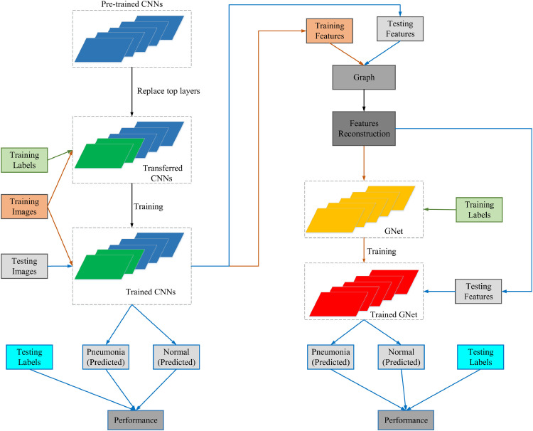
In general classification tasks, features of data are first extracted and then be classified by classifiers in traditional ML methods. In our proposed CGNet framework, there are mainly three individual components that correspond to feature extraction, feature reconstruction and final classification respectively. However, unlike traditional ML methods, which heavily rely on manually-crafted features, our framework extracts high-level abstract features by transferring the state-of-the-art CNNs in the first step. Graph representations are then delved into depth according to features‘ Euclidean distance. Finally, the classifiers are trained with features embedded with graph representation. The data flow of the proposed model under CGnet framework can be seen in Fig. 1 .
Fig. 1.
The flow chart of the proposed framework.
In Fig. 1, the procedures on obtaining trained CNNs is shown in left. The dark greened layers shown in transferred CNNs and trained CNNs are new top layers that replace original top layers in CNNs. The arrows in orange and blue show the flows of the training set and the test set. When implementing our models for pneumonia detection under CGNet framework, we choose CNNs that performed best on the test set as feature extractors. GNet, which takes features combined with graph representations as input, finally classifies images into normal and pneumonia. We will have a detailed illustration of each component as follows.
3.1. Feature extraction by transferred CNNs
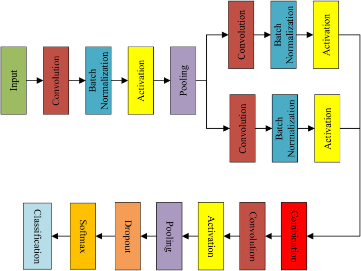
Unlike traditional ML methods that utilize manually-designed algorithms for ad hoc tasks, we use deep- learning-based algorithms that have a higher superiority on generalization. Feature extraction plays a key role in the classification task, which directly determines the overall performance of the following classifiers. Primarily, we implement feature extraction by deploying transfer learning technique. In our feature extraction stage, the state-of-the-art networks are first transferred to the binary classification task by replacing top layers with new layers. After training with the training set, CNNs that can provide preliminary results as well as features. Generally, CNNs are trained on ImageNet (Deng et al., 2009) that give 1000-categories classification results. The general architecture of CNNs is given in Fig. 2 . After transferred the state-of-the-art networks, we chose the CNN that gives the best result on the test set as a feature extractor for following GNet.
Fig. 2.
General architecture of CNNs.
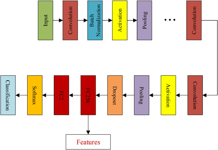
To transfer CNNs pre-trained on ImageNet, we first removed the top layers of CNNs and then added new layers including one dropout layer, one transitional fully-connected layer with 256 channels and the final 2 channel fully-connected layer for classification. Dropout layer is added to prevent overfitting problem during the training session. Information of features would suffer from significant loss if the dimensions of feature shrink rapidly. Therefore, a transitional fully-connected layer is placed on the top of the dropout layer to prohibit heavy information loss. The detailed architecture of transferred CNNs can be seen in Fig. 3 , where FC256 and FC2 stand for two fully-connected layers with 256 and 2 channels respectively. The connection between the final pooling layer and Softmax layer is replaced by the connection between the final pooling layer and newly added dropout layer. After training the transferred networks with pneumonia dataset with a limited number of epochs, the parameters within CNNs are fine-tuned towards the desired parameters that give better representations of the dataset. The details about the acquisition of features under our framework can be found in Algorithm 1 , which includes two states that are network transferring and feature extraction, where the extracted features are analysed for underlying graph representation.
Fig. 3.
Architecture of transferred CNNs. FC256 and FC2 stand for fully connected layers with 256 and 2 channels respectively.
Algorithm 1.
Feature acquisition.
| Stage 1: Network transferring |
| Step 1.1: Load pre-trained state-of-the-art networks; (trained on ImageNet;) |
| Step 1.2: Remove the Softmax layer and classification layer; |
| Step 1.3: Add new layers including dropout, FC256, FC2, new Softmax layers, and new classification layers; |
| Step 1.4: Train new networks on the training set of pneumonia dataset with predefined parameters; |
| Step 1.5: Save trained networks and parameters; |
| Stage 2: Feature extraction |
| Step 2.1: Load trained networks; |
| Step 2.2: Input the dataset to trained networks for feature extraction; |
| Step 2.3: Extract features produced by fully-connected layer FC256. |
3.2. Graph embedded feature reconstruction
We use graph information extracted from features to reconstruct the features. The reason why we do this is that individual feature will be enhanced when reconstructed by neighbour features. Features here refer to features extracted by trained CNNs. To build graphs of features, each feature extracted from each image is taken as a node of the graphs. For efficient computation, features are partitioned into batches. Given the features, where Dis the number of features in the dataset and M is the dimension of the features. Let the batch size to be N, then the number of batches n can be denoted as:
| (4) |
where ⌈ · ⌉ is the ceiling operation. Then F can be rewritten as:
| (5) |
| (6) |
where and . Specifically, f jis the feature extracted by the previous component. For each F i, a corresponding graph Gi that represents the underlying relationship between nodes by the paired variables (Vi, Ei) can be built. Vi stands for the nodes comprised of each feature f j in the batch, while Ei is the edges between nodes. We believe edges exist between each node and its nearest k neighbours when k smallest Euclidean distance found. Ei is represented in a form of the adjacency matrix . Given a node f jand its neighbour the value at the position (j, j + 1) of A i is set to be a positive number that shows two nodes are related. Hence, the key to build Gi is to calculate the adjacency matrix A i (Liang & Bose, 1996). The procedures of graph generation can be seen in Algorithm 2 .
Algorithm 2.
Graph generation.
| Divide features into batches; |
| For each batch of features, let each feature in the batch be the node; |
| Calculate the Euclidean distance between each node to the rest nodes in the graph; |
| Find nearest k neighbours for each node; |
| Assign a positive value at positions that correspond to k neighbours. |
When building graph Gi for each batch of features Fi, we first calculate the distance between each feature to the rest features in the batch. By doing so, we can have a distance matrix Distance . After sorting each row of the acquired Distancein ascending order, the corresponding index matrix Index that records the index of nearest k features in the batch Fi before sortation can be produced. For each row of Ai, the value of one position in the row is set to 1 when the neighbour at the position is found to be one of the nearest k neighbours.
The pseudocode of acquisition of Ai can be found in Algorithm 3 . At the initialization stages, the four variables are initialized as:
| (7) |
| (8) |
| (9) |
| (10) |
Algorithm 3.
Acquisition of adjacency matrix Ai.
| Step 1: Initialization (See Eqs. (7)-10) |
| Initialize adjacency matrix Ai; |
| Initialize distance between features Distance; |
| Initialize variable Sorted_Distance for sorted distance; |
| Initialize variable Index; |
| Step 2: Distance calculation |
| for a = 1:S |
| for b = 1:S |
| if a!=b |
| ; |
| end |
| end |
| end |
| Step 3: Output Ai |
| for a = 1:S |
| ; |
| for c = 1:k |
| ; |
| end |
| end |
| then output Ai. |
Specifically, the Distance is calculated according to:
| (11) |
After we calculated Ai, each feature fj in the batch Fi is reconstructed according to:
| (12) |
is the jth row of , which is normalized adjacency matrix Ai. Therefore, the reconstructed feature batch F′ ican be denoted as:
| (13) |
When considering normalizing Ai, we first calculate a degree matrix D , where:
| (14) |
That is to say:
| (15) |
We then normalize Ai by:
| (16) |
I is the identity matrix. After multiplying with F i, we then have reconstructed feature batch F′ i for classification. For pneumonia detection task, the reconstructed feature batches are input to the proposed GNet in the developed system.
3.3. GNet for classification
We name our classifier as GNet when implementing our system for the detection of pneumonia because the proposed GNet is a single layer graph neural network where inputs are the nodes in the graph and the graph representations of the graph. In more general cases, traditional classifiers including ANN (Artificial Neural Network) and SVM (Support Vector Machine) can be used for classification based on extracted features.
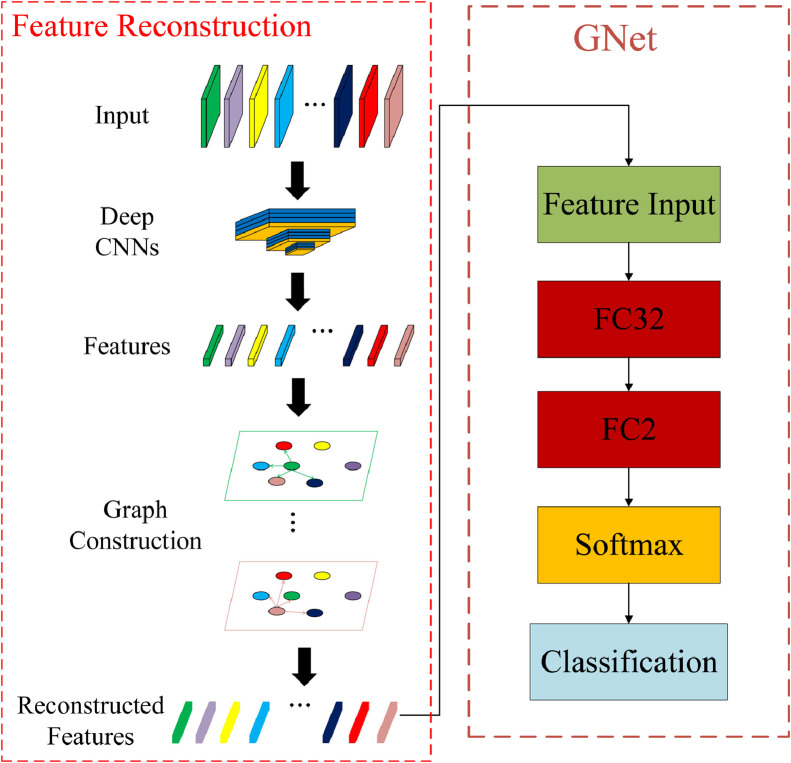
Feature reconstruction procedures and architecture of GNet are shown in Fig. 4 . In feature reconstruction, features mean the features extracted by the trained CNNs. In our scenario, GNet, which has the same structure as traditional ANNs, is different from traditional ANNs on input, where ANNs usually use features extracted with no postprocessing. The main reason why we don't introduce more hidden layers is that extra hidden layers will introduce an even large number of parameters, which could also trigger the overfitting problem. Also, we've obtained most representative features by reconstruction, and therefore only one hidden layer is introduced. The number of input channel is 256.
Fig. 4.
Feature reconstruction and the architecture of GNet.
Given the expected output of batch Fi is FEi and the real output of GNet is FOi, then FOi is:
| (17) |
| (18) |
where
| (19) |
| (20) |
where δ( · ) is the Softmax activation function that can be extended as:
| (21) |
The errors ▵E i between FEi and FOi is:
| (22) |
The weights W and bias b are updated according to stochastic gradient descent with momentum (SGDM) algorithm:
| (23) |
| (24) |
where θ is the momentum rate. W h and b h can be calculated according to the chain-rule. By iteratively updating W, W h, b, and b h, we then have a trained ANN for our binary classification task here. Thereafter, we input each batch feature for the classification. By aggregating all predicted categories of all batches, we then receive classification results for data in the test set. The pseudocode of our proposed framework can be found in Algorithm 4 .
Algorithm 4.
Pseudocode of CGNet framework.
| Loading CNNs pre-trained on ImageNet; |
| Remove top layers and add new top layers for the classification task; |
| Train the modified CNNs on the training dataset; |
| Obtain features through a fully-connected layer whose output size is 1000 from the trained CNNs; |
| Divide features into batches of same sizes; |
| Build graphs in each batch of features; |
| Reconstruct features according to graph information; |
| Train neural networks with reconstructed features; |
| Acquire features for test set by repeat Step 4 to Step 7 on the test set; |
| Test the trained neural networks with the reconstructed test features. |
3.4. Evaluation metrics
To measure the performance of the proposed model, we use common metrics including Sensitivity, Specificity, Accuracy, Precision and F1 score like many other works to measure the performance of our proposed classifier. To calculate the metrics, True Positive (TP), True Negative (TN), False Positive (FP) and False Negative (FN) are introduced.
The higher the TP and TN, the better performance of classifiers that can detect true pneumonia images and normal images; The lower the FP and FN, the fewer mistakes of classifiers that misclassify normal images as pneumonia images and vice versa. The sensitivity is related to TP by:
| (25) |
The specificity, which implies the capability of classifiers on recognition of normal images, can be denoted by TN and FP by:
| (26) |
The overall performance of classifiers is measured by the accuracy:
| (27) |
The Precision measures the percentage of real pneumonia images out of all predicted pneumonia images:
| (28) |
F1 shows the classification ability of the classifiers:
| (29) |
4. Experiment design
In this section, we will briefly go through the details about the datasets (Section 4.1) used in this research, followed by experiment settings (Section 4.2) that gives the details about the experiment configuration. The performance of the transferred networks (Section 4.3) is given before we move to the exploration of batch size N and the number of neighbours k for GNet in Section 4.4. The effectiveness of feature reconstruction and comparison of feature reconstruction methods are given in Section 4.5 and Section 4.6 respectively. We conclude this section by comparing our proposed method with the state-of-the-art methods in Section 4.7.
4.1. Datasets
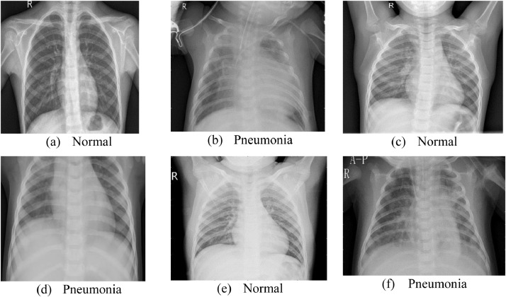
In this research, we validated our proposed feature reconstruction method on two public datasets from two different modalities. We used one cohort that has been confirmed with pneumonia caused by bacteria, which we named it as dataset1. In the dataset1, which is publicly available at (Chest X-Ray Images (Pneumonia) 2020), there are in total 5856 normal and pneumonia X-ray images. To provide a fair comparison platform for different systems, the training set, validation set and the test set have been partitioned beforehand. Examples of normal and pneumonia samples can be seen in Fig. 5 . Details about the dataset1 are shown in Table 1 .
Fig. 5.
Samples of dataset1.
Table 1.
Details of the dataset1.
| Set | Normal | Pneumonia | Total Number |
|---|---|---|---|
| Training | 1341 | 3875 | 5216 |
| Validation | 8 | 8 | 16 |
| Testing | 234 | 390 | 624 |
| Overall | 1583 | 4273 | 5856 |
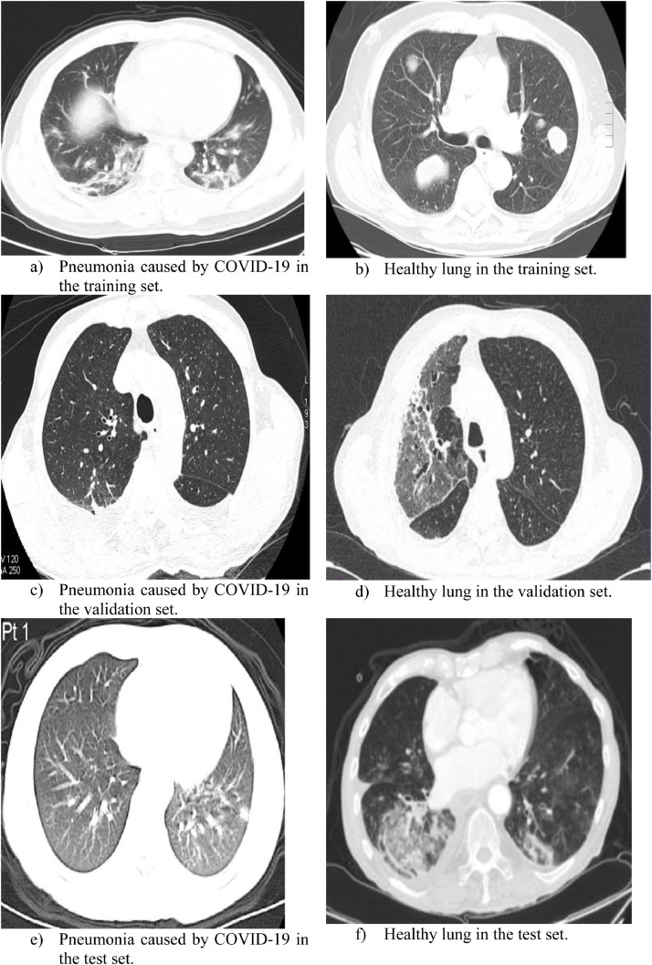
We also examined our proposed method on another public CT-based pneumonia dataset in which the pneumonia was caused by COVID-19 and we named the dataset as dataset2 (Zhao, Zhang, He & Xie, 2020). Some sample images are shown in Fig. 6 . The size of three-channel RGB images varies from 720 × 541 × 3 to 725 × 551 × 3.
Fig. 6.
Sample images from the dataset2.
Compared to images acquired through X-ray instrument, CT lung images show more advantages on image resolutions and fine-grained details. The detailed composition of dataset 2 is shown in Table 2 .
Table 2.
Details of the dataset2.
| Set | Normal | Pneumonia | Total Number |
|---|---|---|---|
| Training | 234 | 191 | 425 |
| Validation | 58 | 60 | 118 |
| Testing | 105 | 98 | 203 |
| Overall | 397 | 349 | 746 |
4.2. Experiment settings
The configuration of this research is a personal laptop with 16 G RAM and GPU GTX1050. As we have to train transferred networks and the following ANN and GNet in a sequence, we have two different sets of parameters. Deep learning toolbox provided by Mathworks is used as the framework. For transferred networks, they are trained for 20 epochs while the initial learning rate is 10−4. Batch size is 8 to prevent system crash due to the memory. We use the stochastic gradient descent with momentum (SGDM) as the optimization method. Also, we have the learning rate halved every 5 epochs to ensure the convergence. When training transferred networks with the training set, images in the training set shuffle at every epoch. Detailed settings can be seen in Table 3 , which remained unchanged during the training process of networks on two datasets.
Table 3.
Training parameters for transferred CNNs.
| Parameters | Value |
|---|---|
| Maximum training epoch | 20 |
| Initial learning rate | 10−4 |
| Batch size | 8 |
| Learning rate drop period | 5 |
| Learning rate drop rate | 0.5 |
| Optimization method | SGDM |
| Shuffle of the train set | Each epoch |
When constructing graphs for reconstruction, the size N of each batch and the number of neighbours k within each batch should be carefully chosen to make sure best performance of GNet can be achieved. When training ANN with features extracted from the transferred networks, we increased the training epochs to be 40 while other parameters have remained unchanged. We use the same parameters throughout the experiments if there are no other specifications. Then we vary N and k to explore the relationship between N, k and the performance of the ANN. Details will be presented in the following sections.
4.3. Performance of the transferred networks
To find out the best-performed state-of-the-art networks that can be transferred to our classification task here, we trained networks including AlexNet (Krizhevsky Alex, 2012), GoogLeNet (Szegedy Christian et al., 2015), SqueezeNet (Iandola et al., 2016), VGG16 (Simonyan Karen, 2014), XceptionNet (Chollet, 2017), ResNet18 (He Kaiming et al., 2016), ResNet101, InceptionV3 (Szegedy, Vanhoucke, Ioffe, Shlens & Wojna, 2016), DenseNet201 (Huang et al., 2017). All of those networks are pre-trained on ImageNet for the 1000-category classification task. To make a fair comparison amongst all of the networks, top layers including FC256, and FC2 are inserted between the Softmax layer and the dropout layer. The original Softmax layer and classification layer are, therefore, replaced by new Softmax layer and a classification layer. The numbers of learnable parameters of the networks introduced are listed in Table 4 .
Table 4.
Numbers of learnable training parameter in the state-of-the-art networks.
| Model name | Number of parameters(Millions) | Number of Layers |
|---|---|---|
| AlexNet | 6.10 | 25 |
| GoogLeNet | 0.70 | 144 |
| SqueezeNet | 0.12 | 68 |
| VGG16 | 13.84 | 41 |
| XceptionNet | 2.29 | 170 |
| ResNet18 | 1.17 | 71 |
| ResNet101 | 4.45 | 347 |
| DenseNet201 | 1.98 | 708 |
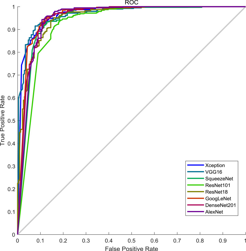
After training with the dataset1, the results of different networks are organized in Table 5 while ROC curves are shown in Fig. 7 .
Table 5.
Performance of state-of-the-art networks on the dataset1.
| Model name | Specificity | Sensitivity | F1 | Precision | AUC | Accuracy |
|---|---|---|---|---|---|---|
| AlexNet | 0.9974 | 0.5000 | 0.6648 | 0.9915 | 0.9747 | 0.8109 |
| GoogLeNet | 0.9949 | 0.4744 | 0.6398 | 0.9823 | 0.9680 | 0..7997 |
| SqueezeNet | 0.9974 | 0.4402 | 0.6095 | 0.9904 | 0.9730 | 0.7885 |
| VGG16 | 1.0000 | 0.3462 | 0.5143 | 1.0000 | 0.9627 | 0.7548 |
| XceptionNet | 0.9872 | 0.6453 | 0.7744 | 0.9679 | 0.9539 | 0.8590 |
| ResNet18 | 0.9974 | 0.5598 | 0.7158 | 0.9924 | 0.9788 | 0.8333 |
| ResNet101 | 1.0000 | 0.5385 | 0.7000 | 1.0000 | 0.9674 | 0.8269 |
| DenseNet201 | 1.0000 | 0.4487 | 0.6195 | 1.0000 | 0.9705 | 0.7933 |
Fig. 7.
ROC curves of the state-of-the-art networks on the test set of dataset1.
On the dataset1, strangely, XceptionNet performed best in all the transferred networks though it was not the deepest one nor newest one. The reasons why XceptionNet performed best could be two folds. One is the architectural novel of XceptionNet. In XceptionNet, shortcut connection technique, which was also being deployed in ResNet and DenseNet, is used besides depthwise separable convolution, which greatly lowers the number of training parameters in the networks. Another possible reason is the size of the input. Note that the input size of XceptionNet is 299 × 299 × 3 while the input size of other networks is no greater than 227 × 227 × 3. However, the original size of the images is greater than 1000 × 1000 × 3. Therefore, XceptionNet experienced much less information loss, which allows more representative features to be extracted. Interestingly, the performance of the networks can be even worse when the depth of networks going deeper, which also requires a longer time for training. Given this, we choose XceptionNet as our feature extractor in this classification task though the performance is still far away from satisfaction.
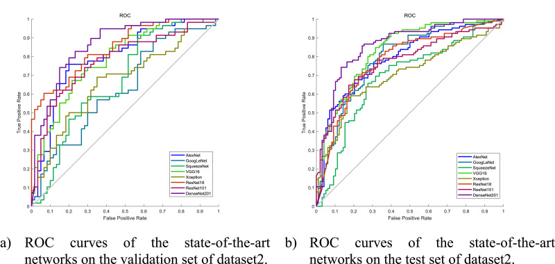
Similarly, we adapted and trained the same state-of-the-art networks on dataset2. The results on the validation set and the test set are shown in Tables 6 and 7 respectively. The ROC curves are shown in Fig. 8 .
Table 6.
Performance of the state-of-the-art networks on the validation set of dataset2.
| Model name | Specificity | Sensitivity | F1 | Precision | AUC | Accuracy |
|---|---|---|---|---|---|---|
| AlexNet | 0.7586 | 0.7333 | 0.7458 | 0.7586 | 0.7957 | 0.7458 |
| GoogLeNet | 0.6552 | 0.4667 | 0.5185 | 0.5833 | 0.6293 | 0.5593 |
| SqueezeNet | 0.5517 | 0.7167 | 0.6667 | 0.6232 | 0.6293 | 0.6356 |
| VGG16 | 0.6724 | 0.7500 | 0.7258 | 0.7031 | 0.7888 | 0.7119 |
| XceptionNet | 0.6897 | 0.6333 | 0.6552 | 0.6786 | 0.6718 | 0.6610 |
| ResNet18 | 0.7069 | 0.7333 | 0.7273 | 0.7213 | 0.8491 | 0.7203 |
| ResNet101 | 0.7759 | 0.6167 | 0.6727 | 0.7400 | 0.7787 | 0.6949 |
| DenseNet201 | 0.8276 | 0.7000 | 0.7500 | 0.8077 | 0.8678 | 0.7627 |
Table 7.
Performance of the state-of-the-art networks on the test set of dataset2.
| Model name | Specificity | Sensitivity | F1 | Precision | AUC | Accuracy |
|---|---|---|---|---|---|---|
| AlexNet | 0.7429 | 0.6735 | 0.6911 | 0.7097 | 0.7920 | 0.7094 |
| GoogLeNet | 0.7619 | 0.6837 | 0.7053 | 0.7283 | 0.7913 | 0.7241 |
| SqueezeNet | 0.7143 | 0.6531 | 0.6667 | 0.6809 | 0.6909 | 0.6847 |
| VGG16 | 0.8095 | 0.6939 | 0.7312 | 0.7727 | 0.8331 | 0.7537 |
| XceptionNet | 0.6381 | 0.7041 | 0.6732 | 0.6449 | 0.7030 | 0.6700 |
| ResNet18 | 0.7619 | 0.6837 | 0.7053 | 0.7283 | 0.7883 | 0.7241 |
| ResNet101 | 0.7714 | 0.6429 | 0.6811 | 0.7241 | 0.7749 | 0.7094 |
| DenseNet201 | 0.8571 | 0.6735 | 0.7374 | 0.8148 | 0.8597 | 0.7685 |
Fig. 8.
ROC curves on dataset2.
Both on the validation set and the test set, DenseNet201 showed the best performance amongst all the state-of-the-art networks. As can be seen from Table 4, the number of learnable parameters in DenseNet201 is not the biggest one, however, the number of layers of DenseNet201 is much greater than that of the rest of the network compared to that of the other state-of-the-art networks. Therefore, DenseNet201 could be benefited from the high density of connections between the layers, which allows more representative features to be learnt. Due to the imaging modality difference between X-ray and CT, XceptionNet, which performed best on the dataset1, turned out to have poor performance on dataset2. Therefore, we used DenseNet201 as the feature extractor when implementing GNet on dataset2.
4.4. The influence of batch size N and number of neighbours k
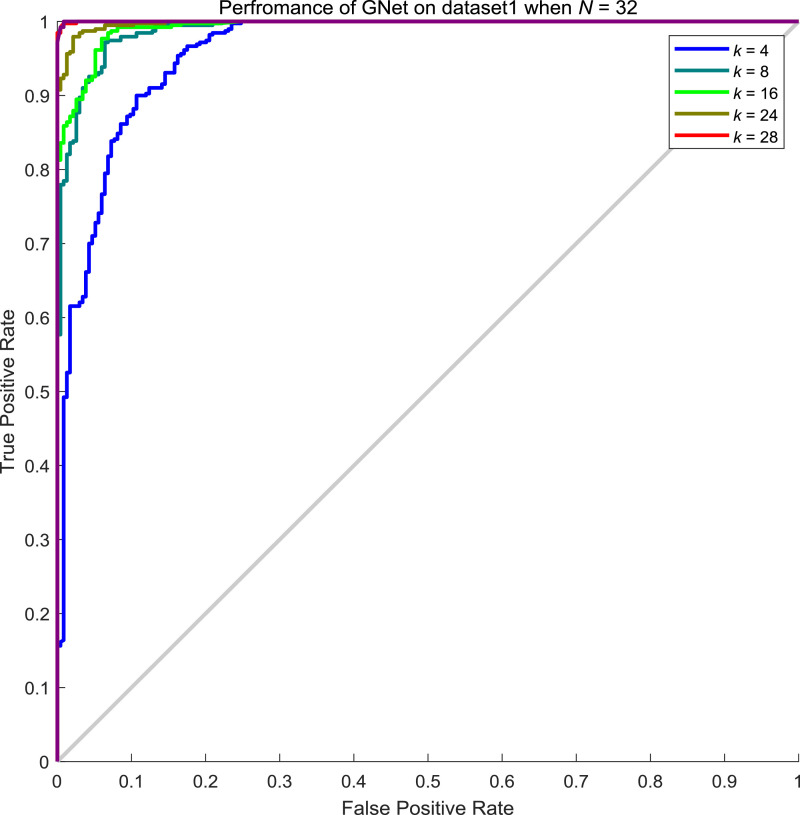
For dataset1, after extracting features by XceptionNet, we then reconstruct features according to generated graphs. However, the batch size N of features and the number k of neighbours being considered are two parameters that are related to the performance of the proposed GNet. Therefore, we explored different sets of N and k to optimize the performance of GNet. In Table 8 , we show a result of GNet when N is 32 while k varies from 4 to 28. In Fig. 9 , the ROC curves of GNet with different configurations are shown. As can be seen, all of the GNets showed an AUC over 0.96 with high AUC at 0.99 achieved. Interestingly, the performance of GNet when k equals to 24 seems to be saturated to that of GNet when k equals to 28
Table 8.
Performance of GNet on the dataset1 when N = 32 and k = 4, 8, 12, 16, 24, 28.
| k | Specificity | Sensitivity | F1 | Precision | AUC | Accuracy |
|---|---|---|---|---|---|---|
| 4 | 1.0000 | 0.4701 | 0.6395 | 1.0000 | 0.9602 | 0.8013 |
| 8 | 1.0000 | 0.7650 | 0.8668 | 1.0000 | 0.9892 | 0.9119 |
| 12 | 1.0000 | 0.5812 | 0.7351 | 1.0000 | 0.9925 | 0.8429 |
| 16 | 0.9949 | 0.9231 | 0.9558 | 0.9908 | 0.9977 | 0.9679 |
| 24 | 1.0000 | 0.9103 | 0.9530 | 1.0000 | 0.9999 | 0.9663 |
| 28 | 1.0000 | 0.9103 | 0.9530 | 1.0000 | 0.9999 | 0.9663 |
Fig. 9.
ROC curves of GNet on the test set of dataset1 when N = 32.
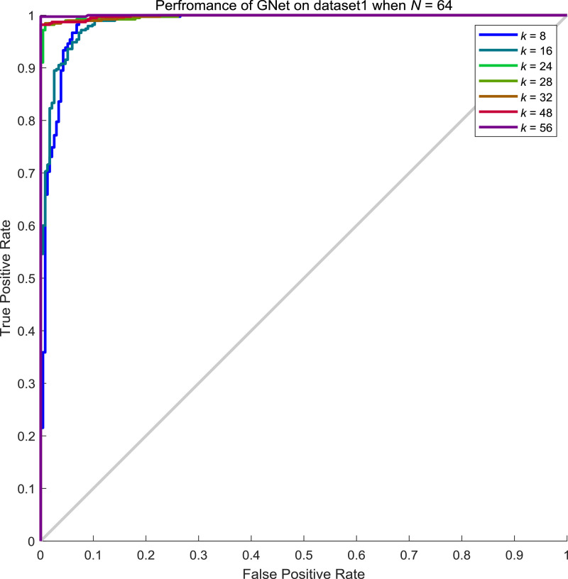
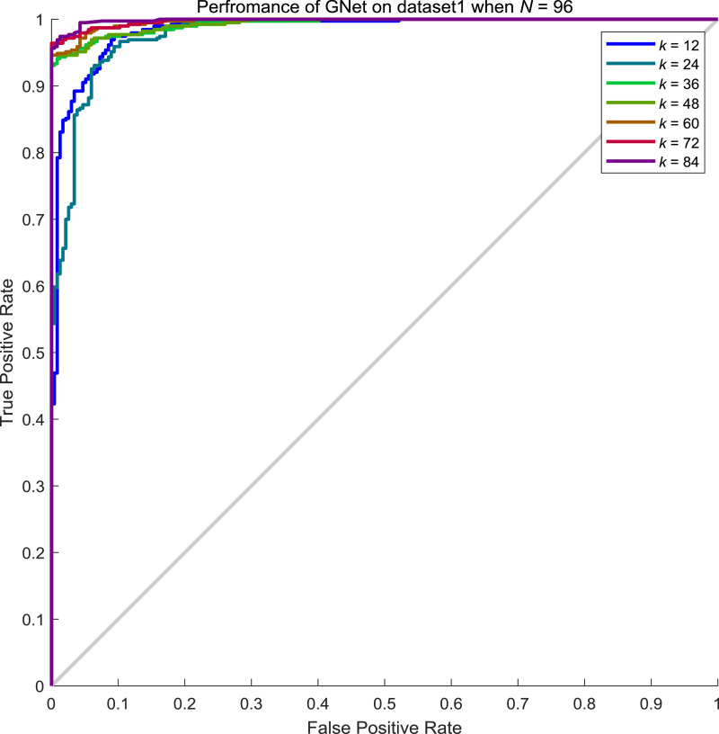
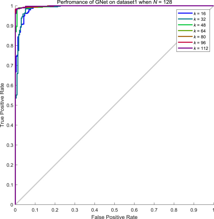
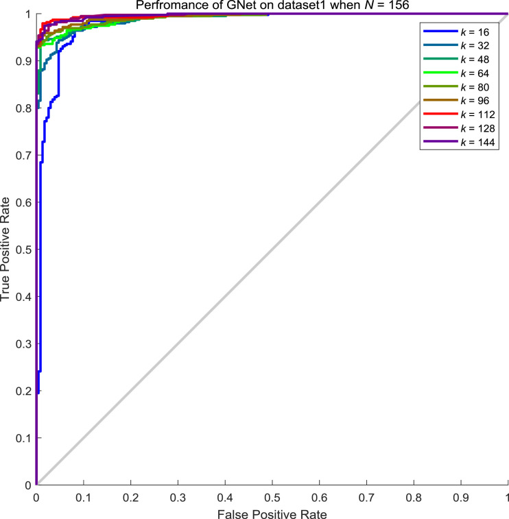
From Table 8, we can conclude that the performance of GNet increases along with the increment of neighbours considered. To explore the influence of batch size N to the performance of GNet, we examined the performance when N is 64, 96, 128 and 156 while k keeps varying. From Tables 9 , Table 10 , Table 11 , and 12 , we showed the performance of GNet when N is 64, 96, 128 and 156 respectively. The corresponding ROC curves are shown in Fig. 10, Fig. 11, Fig. 12, Fig. 13 respectively.
Table 9.
Performance of GNet on the test set of dataset1 when N = 64 and k = 8, 16, 24, 28, 32, 48, 56.
| k | Specificity | Sensitivity | F1 | Precision | AUC | Accuracy |
|---|---|---|---|---|---|---|
| 8 | 1.0000 | 0.6325 | 0.7749 | 1.0000 | 0.9837 | 0.8622 |
| 16 | 1.0000 | 0.4487 | 0.6195 | 1.0000 | 0.9872 | 0.7933 |
| 24 | 0.9923 | 0.8205 | 0.8951 | 0.9846 | 0.9978 | 0.9279 |
| 28 | 0.9974 | 0.7735 | 0.8702 | 0.9945 | 0.9979 | 0.9135 |
| 32 | 0.9974 | 0.7735 | 0.8702 | 0.9945 | 0.9979 | 0.9135 |
| 48 | 0.9872 | 0.9744 | 0.9764 | 0.9785 | 0.9985 | 0.9824 |
| 56 | 0.9436 | 1.0000 | 0.9551 | 0.9141 | 0.9998 | 0.9647 |
Table 10.
Performance of GNet on the test set of dataset1 when N = 96 and k = 12, 24, 36, 48, 60, 72, 84.
| k | Specificity | Sensitivity | F1 | Precision | AUC | Accuracy |
|---|---|---|---|---|---|---|
| 12 | 0.9974 | 0.6795 | 0.8071 | 0.9938 | 0.9842 | 0.8782 |
| 24 | 1.0000 | 0.4615 | 0.6316 | 1.0000 | 0.9793 | 0.7981 |
| 36 | 0.9974 | 0.7094 | 0.8279 | 0.9940 | 0.9932 | 0.8894 |
| 48 | 0.9846 | 0.8462 | 0.9041 | 0.9706 | 0.9936 | 0.9327 |
| 60 | 1.0000 | 0.6923 | 0.8182 | 1.0000 | 0.9964 | 0.8846 |
| 72 | 1.0000 | 0.7179 | 0.8358 | 1.0000 | 0.9974 | 0.8942 |
| 84 | 0.9487 | 1.0000 | 0.9590 | 0.9213 | 0.9985 | 0.9679 |
Table 11.
Performance of GNet on the test set of dataset1 when N = 128 and k = 16, 32, 48, 64, 80, 96, 112.
| k | Specificity | Sensitivity | F1 | Precision | AUC | Accuracy |
|---|---|---|---|---|---|---|
| 16 | 1.0000 | 0.5385 | 0.7000 | 1.0000 | 0.9911 | 0.8269 |
| 32 | 1.0000 | 0.4573 | 0.6276 | 1.0000 | 0.9898 | 0.7965 |
| 48 | 0.9949 | 0.8376 | 0.9074 | 0.9899 | 0.9976 | 0.9359 |
| 64 | 0.9897 | 0.9487 | 0.9652 | 0.9823 | 0.9987 | 0.9744 |
| 80 | 0.9846 | 0.9872 | 0.9809 | 0.9747 | 0.9987 | 0.9856 |
| 96 | 0.9795 | 1.0000 | 0.9872 | 0.9669 | 0.9989 | 0.9872 |
| 112 | 0.9436 | 1.0000 | 0.9551 | 0.9141 | 0.9989 | 0.9647 |
Table 12.
Performance of GNet on the test set of dataset1 when N = 156 and k = 16, 32, 48, 64, 80, 96, 112, 128, 144.
| k | Specificity | Sensitivity | F1 | Precision | AUC | Accuracy |
|---|---|---|---|---|---|---|
| 16 | 0.9974 | 0.6325 | 0.7728 | 0.9933 | 0.9795 | 0.8606 |
| 32 | 0.9949 | 0.7179 | 0.8317 | 0.9882 | 0.9892 | 0.8910 |
| 48 | 0.9974 | 0.5256 | 0.6872 | 0.9919 | 0.9910 | 0.8205 |
| 64 | 0.9923 | 0.8034 | 0.8847 | 0.9843 | 0.9915 | 0.9215 |
| 80 | 0.9692 | 0.9402 | 0.9442 | 0.9483 | 0.9924 | 0.9583 |
| 96 | 0.9462 | 0.9915 | 0.9631 | 0.9170 | 0.9939 | 0.9631 |
| 112 | 0.9282 | 1.0000 | 0.9435 | 0.8931 | 0.9969 | 0.9551 |
| 128 | 0.8974 | 1.0000 | 0.9213 | 0.8540 | 0.9971 | 0.9359 |
| 144 | 0.9256 | 1.0000 | 0.9416 | 0.8897 | 0.9969 | 0.9535 |
Fig. 10.
ROC curves of GNet on the test set of dataset1 when N = 64.
Fig. 11.
ROC curves of GNet on the test set of dataset1 when N = 96.
Fig. 12.
ROC curves of GNet on the test set of dataset1 when N = 128.
Fig. 13.
ROC curves of GNet on the test set of dataset1 when N = 156.
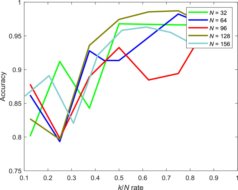
A graph that showed the relationship between batch size N and the number of neighbours k on dataset1 is given in Fig. 14 . As can be seen from Fig. 14, the accuracy increases along with the k when N is small. However, the accuracy seems to be saturated when N is relatively large though k increases. However, it is noticeable that the accuracy imrpoves along with the increament of k/N rate.
Fig. 14.
The relationship between k/N and accuracy on dataset1. (k/N means the ratio between the number of neighbours and batch size N.).
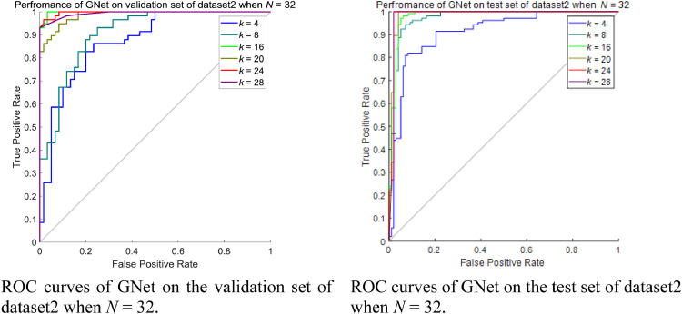
Following a similar pattern, we choose the trained networks that showed the best performance on the dataset2, which was DenseNet201 in this scenario, as the feature extractor. We then vary k and N to specify the best configuration of the proposed GNet, where N ∈ [32, 64, 96], k increases from one-quarter of N to the number close to N by an integer multiple of 4. Table 13 and Table 14 showed the results of GNet on the validation set and the test set of dataset2 when N = 32 respectively. The ROC curves are shown in Fig. 15 .
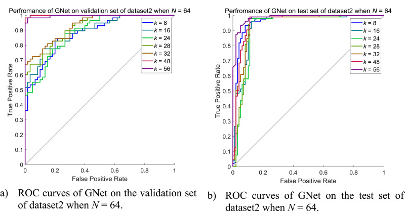
Fig. 16.
Performance of GNet on dataset2 when N = 64.
Table 13.
Performance of GNet on the validation set of dataset2 when N = 32 and k = 4, 8, 16, 20, 24, 28.
| k | Specificity | Sensitivity | F1 | Precision | AUC | Accuracy |
|---|---|---|---|---|---|---|
| 4 | 0.6724 | 0.8833 | 0.8030 | 0.7361 | 0.8744 | 0.7797 |
| 8 | 0.8966 | 0.7833 | 0.8319 | 0.8868 | 0.9080 | 0.8390 |
| 16 | 0.8793 | 1.0000 | 0.9449 | 0.8955 | 0.9980 | 0.9407 |
| 20 | 1.0000 | 0.75000 | 0.8571 | 1.0000 | 0.9862 | 0.8729 |
| 24 | 0.6724 | 1.0000 | 0.8633 | 0.7595 | 0.9971 | 0.8390 |
| 28 | 0.5862 | 1.0000 | 0.8333 | 0.7143 | 0.9980 | 0.7966 |
Table 14.
Performance of GNet on the test set of dataset2 when N = 32 and k = 4, 8, 16, 20, 24, 28.
| k | Specificity | Sensitivity | F1 | Precision | AUC | Accuracy |
|---|---|---|---|---|---|---|
| 4 | 0.8190 | 0.8980 | 0.8585 | 0.8224 | 0.9115 | 0.8571 |
| 8 | 0.9810 | 0.8367 | 0.9011 | 0.9762 | 0.9709 | 0.9113 |
| 16 | 0.9810 | 0.9286 | 0.9529 | 0.9785 | 0.9805 | 0.9557 |
| 20 | 1.0000 | 0.8776 | 0.9348 | 1.0000 | 0.9862 | 0.9409 |
| 24 | 0.7905 | 0.9796 | 0.8889 | 0.8136 | 0.9853 | 0.8818 |
| 28 | 0.9810 | 0.9796 | 0.9796 | 0.9796 | 0.9850 | 0.9803 |
Fig. 15.
Performance of GNet on dataset2 when N = 32.
We also evaluated the performance of GNet when N is 64 while k varies from 8 to 56 by integer multiples of 4. Details about the results on the validation set and the test set of dataset2 can be seen in Tables 15 and 16 while ROC curves are shown in Fig. 16.
Table 15.
Performance of GNet on the validation set of dataset2 when N = 64 and k = 8, 16, 24, 28, 32, 48, 56.
| k | Specificity | Sensitivity | F1 | Precision | AUC | Accuracy |
|---|---|---|---|---|---|---|
| 8 | 0.9138 | 0.5833 | 0.7000 | 0.8750 | 0.8805 | 0.7458 |
| 16 | 0.7759 | 0.8833 | 0.8413 | 0.8030 | 0.8914 | 0.8305 |
| 24 | 0.9655 | 0.5667 | 0.7083 | 0.9444 | 0.8874 | 0.7627 |
| 28 | 0.7759 | 0.8333 | 0.8130 | 0.7937 | 0.9190 | 0.8051 |
| 32 | 0.6897 | 0.9667 | 0.8529 | 0.7632 | 0.9287 | 0.8305 |
| 48 | 0.9310 | 1.0000 | 0.9677 | 0.9375 | 0.9994 | 0.9661 |
| 56 | 0.9828 | 0.9000 | 0.9391 | 0.9818 | 0.9966 | 0.9407 |
Table 16.
Performance of GNet on the test set of dataset2 when N = 64 and k = 8, 16, 24, 28, 32, 48, 56.
| k | Specificity | Sensitivity | F1 | Precision | AUC | Accuracy |
|---|---|---|---|---|---|---|
| 8 | 0.9905 | 0.6122 | 0.7547 | 0.9836 | 0.9560 | 0.8079 |
| 16 | 0.9619 | 0.8571 | 0.9032 | 0.9545 | 0.9365 | 0.9113 |
| 24 | 0.9905 | 0.6633 | 0.7927 | 0.9848 | 0.9218 | 0.8325 |
| 28 | 0.9905 | 0.8776 | 0.9297 | 0.9885 | 0.9325 | 0.9360 |
| 32 | 0.9810 | 0.8878 | 0.9305 | 0.9775 | 0.9457 | 0.9360 |
| 48 | 0.9905 | 0.8367 | 0.9061 | 0.9880 | 0.9565 | 0.9163 |
| 56 | 1.0000 | 0.6531 | 0.7901 | 1.0000 | 0.9565 | 0.8325 |
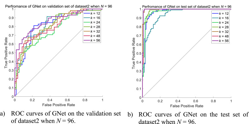
Due to the limited number of images in the validation set on dataset2, the maximum N is chosen to be 96 instead of 128 on dataset1. The detailed results of GNet on the validation set and the test set when N = 96 are shown in Tables 17 and 18 while the corresponding ROC curves are shown in Fig. 17 .
Table 17.
Performance of GNet on the validation set of dataset2 when N = 96 and k = 12, 16, 24, 32, 48, 64, 80.
| k | Specificity | Sensitivity | F1 | Precision | AUC | Accuracy |
|---|---|---|---|---|---|---|
| 12 | 0.8276 | 0.7000 | 0.7500 | 0.8077 | 0.8236 | 0.7627 |
| 16 | 0.7414 | 0.6667 | 0.6957 | 0.7273 | 0.8336 | 0.7934 |
| 24 | 0.7586 | 0.5500 | 0.6168 | 0.7021 | 0.7667 | 0.6525 |
| 32 | 0.7586 | 0.6833 | 0.7130 | 0.7455 | 0.8034 | 0.7203 |
| 48 | 0.7241 | 0.6822 | 0.7009 | 0.7193 | 0.8167 | 0.7034 |
| 64 | 0.4138 | 0.9667 | 0.7632 | 0.6304 | 0.8037 | 0.6949 |
| 80 | 0.8621 | 0.6167 | 0.7048 | 0.8222 | 0.8609 | 0.7373 |
Table 18.
Performance of GNet on the test set of dataset2 when N = 96 and k = 12, 16, 24, 28, 32, 48, 64, 80.
| k | Specificity | Sensitivity | F1 | Precision | AUC | Accuracy |
|---|---|---|---|---|---|---|
| 12 | 0.9810 | 0.8469 | 0.9071 | 0.9765 | 0.9680 | 0.9163 |
| 16 | 0.9524 | 0.7347 | 0.8229 | 0.9351 | 0.9352 | 0.8473 |
| 24 | 0.9810 | 0.7653 | 0.8571 | 0.9740 | 0.9736 | 0.8768 |
| 32 | 0.9810 | 0.9184 | 0.9474 | 0.9783 | 0.9857 | 0.9507 |
| 48 | 1.0000 | 0.8878 | 0.9405 | 1.0000 | 0.9979 | 0.9458 |
| 64 | 0.9333 | 0.9898 | 0.9604 | 0.9327 | 0.9935 | 0.9606 |
| 80 | 1.0000 | 0.9796 | 0.9897 | 1.0000 | 0.9948 | 0.9901 |
Fig. 17.
Performance of GNet on dataset2 when N = 96.
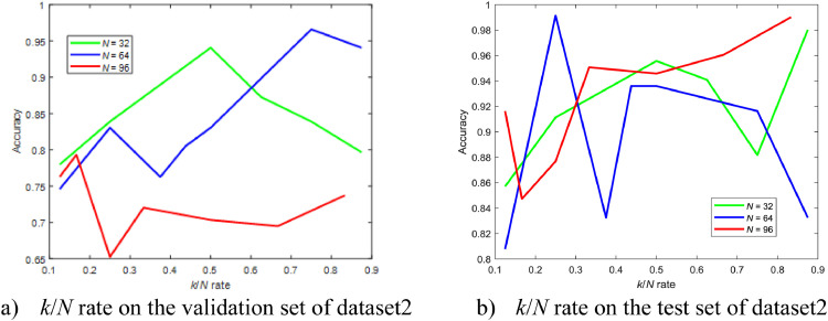
Similarly, we drew graphs that represent the relationship between the performance and k/N rate on the validation set and the test set of dataset2 as can be seen in Fig. 18 .
Fig. 18.
The relationship between k/N rate and Accuracy on dataset2.
As can be seen, the best configuration of GNet on the validation set and the test set are quite different. The performance of GNet fluctuates when k and N are not optimal. Also, due to the limited number of images, a greater number of N doesn't guarantee high performance. However, a rough conclusion can be drawn from Fig. 18 is that when k/N is greater than or close to 0.8 an overall higher performance can be found. A similar conclusion can be found in Fig. 14.
4.5. Effectiveness of feature reconstruction
To evaluate the performance of the proposed method on the detection of pneumonia, we then directly trained XceptionNet with the dataset1 and used the trained XceptionNet as the feature extractor. ANN with the same structure as our GNet is used as the classifier. To validate the effectiveness of feature reconstruction on dataset1, we also examined the performance of ANN when the input is originally extracted features by XceptionNet. Besides, SVM and Decision Tree, two classical supervised classifiers, have been introduced to make comparisons with our proposed model. To avoid confusion, we name ANN trained by original features as ANNraw. Two networks are trained with the same training parameters. The classification results of the two trained networks are given in Table 19 .
Table 19.
Performance of networks feed with different features on dataset1.
| Model name | Specificity | Sensitivity | F1 | Precision | Accuracy |
|---|---|---|---|---|---|
| ANNraw | 0.9385 | 0.7949 | 0.8378 | 0.8857 | 0.8846 |
| SVM | 0.9821 | 0.5897 | 0.7282 | 0.9517 | 0.8349 |
| Decision Tree | 0.9769 | 0.5470 | 0.6900 | 0.9343 | 0.8157 |
| GNet (N = 32, k = 16) | 0.9949 | 0.9231 | 0.9558 | 0.9908 | 0.9679 |
| GNet (N = 64, k = 48) | 0.9872 | 0.9744 | 0.9764 | 0.9785 | 0.9824 |
| GNet (N = 96, k = 84) | 0.9487 | 1.0000 | 0.9590 | 0.9213 | 0.9679 |
| GNet (N = 128, k = 96) | 0.9846 | 0.9915 | 0.9831 | 0.9748 | 0.9872 |
| GNet (N = 156, k = 96) | 0.9462 | 0.9915 | 0.9631 | 0.9170 | 0.9631 |
Parameters in the parenthesis mean the given parameters are used to train GNet. As can be seen, the networks GNet trained with reconstructed features performed much better than the network trained with original features extracted by XceptionNet. Though batch size N and k varies, the accuracy showed a consistent gain compared to the results given by ANNraw. When it comes to computational costs on training two networks, our GNet takes a longer time because of graph construction and graph-feature combination process during feature reconstruction. However, our proposed GNet becomes more advantageous in the prediction phase as the network allows simultaneous classification for multiple images. Considering the computational capability of our laptop, the cost is still expedient. Therefore, we believe the proposed feature reconstruction method will be transplantable to other machines as well. Therefore, we believe our reconstruction method is effective to improve the performance of ANN.
On dataset2, DenseNet201 showed the best performance amongst all of the state-of-the-art networks. Hence, the input of ANN and GNet thereby are the features extracted by DenseNet201.The same architecture of ANN and GNet is employed when making the comparison. As can be seen in Table 20 , the performance of GNet is significantly higher than ANN and SVM.
Table 20.
Performance of networks feed with different features on the test set of dataset2.
| Model name | Specificity | Sensitivity | F1 | Precision | Accuracy |
|---|---|---|---|---|---|
| ANNraw | 0.7810 | 0.6633 | 0.6989 | 0.7386 | 0.7241 |
| SVM | 0.8857 | 0.7347 | 0.7912 | 0.8571 | 0.8128 |
| Decision Tree | 0.8286 | 0.6224 | 0.6893 | 0.7722 | 0.7291 |
| GNet (N = 32, k = 28) | 0.9810 | 0.9796 | 0.9796 | 0.9796 | 0.9803 |
| GNet (N = 64, k = 28) | 0.9905 | 0.8776 | 0.9297 | 0.9885 | 0.9360 |
| GNet (N = 96, k = 80) | 1.0000 | 0.9796 | 0.9897 | 1.0000 | 0.9901 |
4.6. Comparison of feature reconstruction methods
In this section, we compared our proposed feature reconstruction method with PCA-based feature reconstruction method. The eigenvalues and eigenvectors are calculated and selected in an descending order. For two datasets, we ensure that the selected components are able to explain more than 98% of all variability. Therefore, the dimensions of features from two datasets have been reduced from 256 to 152 and 131 respectively. We then trained classifiers including ANN, SVM and decision tree based on the features reconstructed by PCA. Also, we recontructed the features from two datasets based on our graph-knowledge reconstruction method. For simplicity, we choose N to be 32 while k remains to be 16.
As can be seen from Tables 19 and 21 , the performance of ANN decreased slightly while the performance of SVM and decision tree increases. A contradictory conclusion can be drawn from Table 22 that SVM and decision tree performed even worse while the performance of ANN has been improved significantly. Therefore, we may roughly conclude that both PCA-based reconstruction method and our method failed to significantly improve the performance of SVM and decision tree but our method indeed improves the specificity to 1.
Table 21.
Performance of classifiers when input is reconstructed by PCA on the test set of dataset1.
| Model name | Specificity | Sensitivity | F1 | Precision | Accuracy |
|---|---|---|---|---|---|
| ANN | 0.9385 | 0.7778 | 0.8273 | 0.8835 | 0.8782 |
| SVM | 0.9821 | 0.5940 | 0.7316 | 0.9521 | 0.8365 |
| Decision Tree | 0.9846 | 0.6026 | 0.7402 | 0.9592 | 0.8413 |
Table 22.
Performance of classifiers when input is reconstructed by our method on the test set of dataset1.
| Model name | Specificity | Sensitivity | F1 | Precision | Accuracy |
|---|---|---|---|---|---|
| ANN | 0.9949 | 0.9231 | 0.9558 | 0.9908 | 0.9679 |
| SVM | 1.0000 | 0.5427 | 0.7036 | 1.0000 | 0.8285 |
| Decision Tree | 1.0000 | 0.4701 | 0.6395 | 1.0000 | 0.8013 |
On dataset2, we just repeated the same procedures and presented the results in Tables 23 and 24 respectively. Note that the size of the input of ANN has been adjusted to 131 correspondingly. As can be seen, the performance of SVM remains unchanged when PCA is used while our method harmed the performance of SVM. For the decision tree, both methods improved the performance of the decision tree. Based on the results from two datasets, we are convinced that our feature reconstruction method shows great advantage on the improving the performance of ANN while how to improve the performance of SVM and decision tree by our method remains to be explored.
Table 23.
Performance of classifiers when input is reconstructed by PCA on the test set of dataset2.
| Model name | Specificity | Sensitivity | F1 | Precision | Accuracy |
|---|---|---|---|---|---|
| ANN | 0.8095 | 0.5510 | 0.6279 | 0.7297 | 0.6847 |
| SVM | 0.8857 | 0.7347 | 0.7912 | 0.8571 | 0.8128 |
| Decision Tree | 0.9333 | 0.5816 | 0.7037 | 0.8906 | 0.7635 |
Table 24.
Performance of classifiers when input is reconstructed by our method on the test set of dataset2.
| Model name | Specificity | Sensitivity | F1 | Precision | Accuracy |
|---|---|---|---|---|---|
| ANN | 0.9810 | 0.9286 | 0.9529 | 0.9785 | 0.9557 |
| SVM | 1.0000 | 0.2347 | 0.3802 | 1.0000 | 0.6305 |
| Decision Tree | 0.9429 | 0.6122 | 0.7317 | 0.9091 | 0.7833 |
4.7. Comparison of state-of-the-art methods
Considerable works are focusing on designing high accuracy systems for the detection of pneumonia. To provide a fair comparison, we compared our method to methods that have been validated on the same datasets. For pneumonia caused by common bacteria and virus, the performance of different methods is shown in Table 25 .
Table 25.
Methods of pneumonia detection.
| Model name | Specificity | Sensitivity | Precision | Accuracy |
|---|---|---|---|---|
| Liang (Liang & Zheng, 2019) | 0.9549 | 0.9670 | 0.8910 | 0.9050 |
| Wang[22](Wang and Xia 2018) | 0.9949 | 0.9017 | 0.9906 | 0.9599 |
| Rajourkar[3](Rajpurkar, Irvin et al. 2017) | 0.9795 | 0.9359 | 0.9648 | 0.9631 |
| Kermany[42] Kermany et al., 2018 | 0.9872 | 0.9615 | 0.9783 | 0.9776 |
| Islam[4](Islam, Wijewickrema et al.) | 0.9918 | 0.9880 | 0.9918 | 0.9899 |
| Ours method | 0.9846 | 0.9915 | 0.9748 | 0.9872 |
Sensitivity measures the ability of proposed methods on making correct diagnostic results on sick people as patients. Compared to high specificity, high sensitivity is of even greater significance, because healthy people misdiagnosed as the sick suffers much lower risk than patients misdiagnosed as healthy people. As can be seen, our method surpassed the majority of the state-of-the-art methods while our method achieved the highest sensitivity, which means our method shows the stronger capability of detecting pneumonia images.
(The higher the sensitivity the better performance of the proposed methods on detecting real pneumonia images)
To provide a fair comparison with methods based on chest CT images, we also compared our method with the state-of-the-art methods. Detailed results can be seen in Table 26 .
Table 26.
Methods of pneumonia detection caused by COVID-19.
| Model name | Specificity | Sensitivity | Precision | Accuracy |
|---|---|---|---|---|
| Zhao (Zhao et al., 2020) | – | – | – | 0.89 |
| Wu (Wu et al., 2020) | 0.93 | 0.95 | – | 0.93 |
| Jaiswal (Jaiswal, Gianchandani, Singh, Kumar & Kaur, 2020) | 0.96 | – | 0.96 | 0.96 |
| Loey [45] Loey, Manogaran & Khalifa, 2020. | 0.88 | 0.78 | 0.85 | 0.83 |
| He [46] (He, Yang et al. 2020) | – | – | – | 0.86 |
| Our method | 1.0000 | 0.98 | 1.0000 | 0.99 |
(The higher the sensitivity the better performance of the proposed methods on detecting real pneumonia images)
5. Discussion
In this paper, we proposed a novel classifier for the detection of pneumonia based on X-ray and CT images. The proposed feature reconstruction method greatly improved the performance of the neural network with simple architectures. Before inputting images to all models, preprocessing methods are applied to adapt the images for the models. As the sizes of images in the dataset may vary, images are resized for different networks to meet the size requirement of input. Also, the images are not squared while the original height and width of images are greater than 1000 pixels. Therefore, distortion may be introduced due to image resizing. Though XceptionNet performed best amongst all CNNs when dataset1 was concerned, it is, however, could be the larger input images that allow more features to be extracted. In datatset1, images are one-channel grey-scale images. Consequently, images in datasets are converted to three-channel RGB images. For CT-based images in dataset2, DenseNet201, which could be benefited from the rich connections between layers, showed the best performance amongst all of the networks. Except for the procedures mentioned above, no other data augmentation methods are involved. As for similarity measurement in the graph generation process, many other methods can be applied. However, Euclidean distance is the most straightforward way to quantify the difference between features. When reconstructing features, the feature to be reconstructed can be reconstructed by the top k nearest neighbours found. However, the performance of reconstruction could be significantly affected by the distribution of features in the same batch. Therefore, we choose to include the original feature as one of the top k nearest neighbours and therefore mitigate the influence brought by distributions of features. Graph construction and graph-feature combination are the two most important procedures during the process of feature reconstruction. However, these two procedures bring no significant computational costs both in training and prediction period. In general, the validation set is used to validate the performance of the proposed classifiers. However, the validation set in the dataset involved is too small to act as a useful validation set. Therefore, the dataset is suggested to repartition to form real useful validation set.
6. Conclusion
In this paper, we proposed a novel deep learning model for the detection of pneumonia by integrating graph knowledge for feature reconstruction. We hypothesise that features will be more representative if they are reconstructed by neighbours. Based on this, we proposed a graph-based reconstruction method, which turns out to be simple yet effective. If we consider the reconstruction as a component in the following GNet, then the proposed GNet turns into a simple graph neural network with only one layer. Experiments on a large dataset showed the high performance of the proposed feature reconstruction method and the proposed model, whose performance surpassed the state-of-the-art methods. The conclusion is also supported by the results on a public COVID-19 CT-image dataset, where we achieved 99% accuracy.
However, some limitations of this research remain and will be listed as our future work. The sizes of datasets are still very small to produce more convincing results. The construction of the graph and the reconstruction of features are vital parts of our methods. However, there are also more details remain to be explored. For example, we chose a batch size N that is smaller than the dimensions of the input of ANN throughout all the experiments. What if we choose an even larger N that is greater than the dimension of the input? Also, the design of transitional fully connected layers and optimization of the ANN architecture remains to be further explored. However, ANN showed higher priority to other classifiers such as SVM and decision tree. Nevertheless, these details will be implemented in our future work.
CRediT authorship contribution statement
Xiang Yu: Conceptualization, Methodology, Software, Validation, Data curation. Shui-Hua Wang: Resources, Investigation, Project administration, Funding acquisition. Yu-Dong Zhang: Resources, Formal analysis, Investigation, Data curation, Writing - review & editing, Supervision, Project administration, Funding acquisition.
Acknowledgement
Xiang Yu holds a CSC scholarship with the University of Leicester. The paper was partially supported by Royal Society International Exchanges Cost Share Award, UK (RP202G0230); Hope Foundation for Cancer Research, UK (RM60G0680); Medical Research Council Confidence in Concept Award, UK (MC_PC_17171); British Heart Foundation Accelerator Award, UK; Fundamental Research Funds for the Central Universities (CDLS-2020-03); Key Laboratory of Child Development and Learning Science (Southeast University), Ministry of Education; Guangxi Key Laboratory of Trusted Software (kx201901).
References
- Abbas, A., Abdelsamea, M.M., .& Gaber, M.M. (.2020)"Classification of COVID-19 in chest X-ray images using DeTraC deep convolutional neural network," arXiv preprint arXiv:2003.13815. [DOI] [PMC free article] [PubMed]
- Adhikari N.C.D. Infection severity detection of CoVID19 from X-Rays and CT scans using artificial intelligence. International Journal of Computer (IJC) 2020;38:73–92. [Google Scholar]
- Apostolopoulos I.D., Mpesiana T.A. Covid-19: Automatic detection from x-ray images utilizing transfer learning with convolutional neural networks. Physical and Engineering Sciences in Medicine, 43, 2020:635-640. doi: 10.1007/s13246-020-00865-4. [DOI] [PMC free article] [PubMed] [Google Scholar]
- Behzadi P., Ranjbar R., Alavian S.M. Nucleic acid-based approaches for detection of viral hepatitis. Jundishapur Journal of Microbiology. 2014;8:e17449. doi: 10.5812/jjm.17449. e17449. [DOI] [PMC free article] [PubMed] [Google Scholar]
- Bukhari, S.U.K., Bukhari, S.S.K., Syed, A., & SHAH, S.S.H. (2020)"The diagnostic evaluation of convolutional neural network (CNN) for the assessment of chest X-ray of patients infected with COVID-19," medRxiv: 2020.2003.2026.20044610.
- Chen X., Chen Y., Liu H., Goldmacher G., Roberts C., Maria D. PIN92 Pediatric bacterial pneumonia classification through chest X-rays using transfer learning. Value in Health. 2019;22:S209–S210. [Google Scholar]
- (2020,. 2020). Chest X-Ray Images (Pneumonia). Available: https://www.kaggle.com/paultimothymooney/chest-xray-pneumonia.
- Chollet F. Proceedings of the IEEE conference on computer vision and pattern recognition. 2017. Xception: Deep learning with depthwise separable convolutions; pp. 1251–1258. [Google Scholar]
- Chowdhury, M.E., .Rahman, T., Khandakar, A., Mazhar, R., Kadir, M.A., .& Mahbub, Z.B. e.t al.,(2020) "Can AI help in screening viral and COVID-19 pneumonia?," arXiv preprint arXiv:2003.13145.
- Chung H., Park J.G., Jung H.Y. Rank‐weighted reconstruction feature for a robust deep neural network‐based acoustic model. ETRI Journal. 2019;41:235–241. [Google Scholar]
- Deng J., Dong W., Socher R., Li L.-.J., Li K., Fei-Fei L. IEEE conference on computer vision and pattern recognition, 2009. 2009. Imagenet: A large-scale hierarchical image database; pp. 248–255. [Google Scholar]
- Fang Y., Zhang H., Xie J., Lin M., Ying L., Pang P. Sensitivity of chest CT for COVID-19: Comparison to RT-PCR. Radiology. 2020 doi: 10.1148/radiol.2020200432. [DOI] [PMC free article] [PubMed] [Google Scholar]
- He Kaiming Z.X., Shaoqing Ren, Jian S. Proceedings of the IEEE conference on computer vision and pattern recognition. 2016. Deep residual learning for image recognition; pp. 770–778. [Google Scholar]
- He K., Zhang X., Ren S., Sun J. Proceedings of the IEEE international conference on computer vision. 2015. Delving deep into rectifiers: Surpassing human-level performance on imagenet classification; pp. 1026–1034, Las Vegas Nevada. [Google Scholar]
- He K., Zhang X., Ren S., Sun J. Proceedings of the IEEE conference on computer vision and pattern recognition. 2016. Deep residual learning for image recognition; pp. 770–778. [Google Scholar]
- He, X., Yang, X., Zhang, S., Zhao, J., Zhang, Y., & Xing, E. et al.,(2020) "Sample-efficient deep learning for COVID-19 diagnosis based on CT scans," medRxiv,.doi: 10.1101/2020.04.13.20063941.
- Huang G., Liu Z., Van Der Maaten L., Weinberger K.Q. Proceedings of the IEEE conference on computer vision and pattern recognition (CVPR) 2017. Densely connected convolutional networks; pp. 4700–4708, Honolulu Hawaii, USA. [Google Scholar]
- Iandola, F.N., .Han, S., Moskewicz, M.W., .Ashraf, K., Dally, W.J., .& a. p. a. Keutzer, K.J. (.2016)."SqueezeNet: AlexNet-level accuracy with 50x fewer parameters and< 0.5MB model size,"ArXiv abs/1602.07360.
- Islam, K.T., .Wijewickrema, S., Collins, A., & O'Leary, S. (2020)."A deep transfer learning framework for pneumonia detection from chest X-ray images.", pp. 286-293. 10.5220/0008927002860293.
- Jaiswal A., Gianchandani N., Singh D., Kumar V., Kaur M. Classification of the COVID-19 infected patients using DenseNet201 based deep transfer learning. Journal of Biomolecular Structure and Dynamics. 2020:1–8. doi: 10.1080/07391102.2020.1788642. [DOI] [PubMed] [Google Scholar]
- Jia Y., Shelhamer E., Donahue J., Karayev S., Long J., Girshick R. Caffe: Convolutional architecture for fast feature embedding. Proceedings of the 22nd ACM international conference on multimediaet al. 2014:675–678, doi: 10.1145/2647868.2654889. [Google Scholar]
- Joaquin, A. (2020)."Using deep learning to detect pneumonia caused by NCOV‐19 from X‐ray images," ed, available at: https://towardsdatascience.com/using-deep-learning-to-detect-ncov-19-from-x-ray-images-1a89701d1acd.
- Kermany D.S., Goldbaum M., Cai W., Valentim C.C., Liang H., Baxter S.L. Identifying medical diagnoses and treatable diseases by image-based deep learning. Cell. 2018;172:1122–1131. doi: 10.1016/j.cell.2018.02.010. e9. [DOI] [PubMed] [Google Scholar]
- Koo H.J., Lim S., Choe J., Choi S.-.H., Sung H., Do K.-.H. Radiographic and CT features of viral pneumonia. Radiographics : A Review Publication of the Radiological Society of North America, Inc. 2018;38:719–739. doi: 10.1148/rg.2018170048. 05/01, 2018. [DOI] [PubMed] [Google Scholar]
- Krizhevsky Alex S.I., H.G. E . Advances in neural information processing systems. 2012. Imagenet classification with deep convolutional neural networks; pp. 1097–1105. [Google Scholar]
- Li K., Wu J., Wu F., Guo D., Chen L., Fang Z. The clinical and chest CT features associated with severe and critical COVID-19 pneumonia. Investigative Radiology. 2020;55 doi: 10.1097/RLI.0000000000000672. [DOI] [PMC free article] [PubMed] [Google Scholar]
- Li Z., Zhang Z., Qin J., Zhang Z., Shao L. Discriminative fisher embedding dictionary learning algorithm for object recognition. IEEE Transactions on Neural Networks and Learning Systems. 2019 doi: 10.1109/TNNLS.2019.2910146. [DOI] [PubMed] [Google Scholar]
- Liang G., Zheng L. A transfer learning method with deep residual network for pediatric pneumonia diagnosis. Computer Methods and Programs in Biomedicine. 2019 doi: 10.1016/j.cmpb.2019.06.023. [DOI] [PubMed] [Google Scholar]
- Liang P., Bose N. Mac Graw-Hill; 1996. Neural network fundamentals with graphs, algorithms, and applications. [Google Scholar]
- Loey, M., Manogaran, G., & Khalifa, N.E.M. (2020)."A deep transfer learning model with classical data augmentation and cgan to detect covid-19 from chest ct radiography digital images,", Preprints 2020040252. [DOI] [PMC free article] [PubMed]
- Malagón-Borja L., Fuentes O. Object detection using image reconstruction with PCA. Image and Vision Computing. 2009;27:2–9. [Google Scholar]
- Rajpurkar, P., Irvin, J., Zhu, K., Yang, B., Mehta, H., & Duan, T. et al.,(2017) "Chexnet: Radiologist-level pneumonia detection on chest x-rays with deep learning," arXiv preprint arXiv:1711.05225.
- Ronneberger O., Fischer P., Brox T. International conference on medical image computing and computer-assisted intervention. 2015. U-net: Convolutional networks for biomedical image segmentation; pp. 234–241. [Google Scholar]
- Shen H.T., Zhu X., Zhang Z., Wang S.-.H., Chen Y., Xu X. Heterogeneous data fusion for predicting mild cognitive impairment conversion. Information Fusion. 2021;66:54–63. 2021/02/01/ [Google Scholar]
- Simonyan Karen, Z.A. (.2014)"Very deep convolutional networks for large-scale image recognition," arXivpreprint arXiv:1409.1556.
- Szegedy Christian L.W., Jia Yangqing, Sermanet Pierre, Reed Scott, Anguelov Dragomir, Erhan Dumitru. Proceedings of the IEEE conference on computer vision and pattern recognition. 2015. Going deeper with convolutions; pp. 1–9. [Google Scholar]
- Szegedy C., Vanhoucke V., Ioffe S., Shlens J., Wojna Z. Proceedings of the IEEE conference on computer vision and pattern recognition. 2016. Rethinking the inception architecture for computer vision; pp. 2818–2826, Las Vegas Nevada, USA. [Google Scholar]
- Wang, H., & Xia, Y. (2018)"Chestnet: A deep neural network for classification of thoracic diseases on chest radiography," arXiv preprint arXiv:1807.03058. [DOI] [PubMed]
- Wang, S., Kang, B., Ma, J., Zeng, X., Xiao, M., & Guo, J. et al.,(2020) "A deep learning algorithm using CT images to screen for corona virus disease (COVID-19)," MedRxiv,, doi: 10.1101/2020.02.14.20023028. [DOI] [PMC free article] [PubMed]
- Wen J., Zhang Z., Zhang Z., Fei L., Wang M. Generalized incomplete multiview clustering with flexible locality structure diffusion. IEEE Transactions on Cybernetics. 2020 doi: 10.1109/TCYB.2020.2987164. [DOI] [PubMed] [Google Scholar]
- Wu, Y.-.H., Gao, S.-.H., Mei, J., Xu, J., Fan, D.-.P., & Zhao, C.-.W. et al.,(2020) "JCS: An explainable COVID-19 diagnosis system by joint classification and segmentation," arXiv preprint arXiv:2004.07054. [DOI] [PubMed]
- Zhang Z., Lai Z., Huang Z., Wong W.K., Xie G.-.S., Liu L. Scalable supervised asymmetric hashing with semantic and latent factor embedding. IEEE Transactions on Image Processing. 2019;28:4803–4818. doi: 10.1109/TIP.2019.2912290. [DOI] [PubMed] [Google Scholar]
- Zhang Z., Liu L., Luo Y., Huang Z., Shen F., Shen H.T. Inductive structure consistent hashing via flexible semantic calibration. IEEE Transactions on Neural Networks and Learning Systems. 2020 doi: 10.1109/TNNLS.2020.3018790. [DOI] [PubMed] [Google Scholar]
- Zhang Z., Liu L., Shen F., Shen H.T., Shao L. Binary multi-view clustering. IEEE Transactions on Pattern Analysis and Machine Intelligence. 2018;41:1774–1782. doi: 10.1109/TPAMI.2018.2847335. [DOI] [PubMed] [Google Scholar]
- Zhao, J., Zhang, Y., He, X., & Xie, P. (2020)"COVID-CT-Dataset: A CT scan dataset about COVID-19," arXiv preprint arXiv:2003.13865.
- Zhao Z.-.Q., Zheng P., Xu S.-t., Wu X. Object detection with deep learning: A review. IEEE Transactions on Neural Networks and Learning Systems. 2019 doi: 10.1109/TNNLS.2018.2876865. [DOI] [PubMed] [Google Scholar]


