Abstract
Pixelwise segmentation of the left ventricular (LV) myocardium and the four cardiac chambers in 2-D steady state free precession (SSFP) cine sequences is an essential preprocessing step for a wide range of analyses. Variability in contrast, appearance, orientation, and placement of the heart between patients, clinical views, scanners, and protocols makes fully automatic semantic segmentation a notoriously difficult problem. Here, we present Ω-Net (Omega-Net): A novel convolutional neural network (CNN) architecture for simultaneous localization, transformation into a canonical orientation, and semantic segmentation. First, an initial segmentation is performed on the input image; second, the features learned during this initial segmentation are used to predict the parameters needed to transform the input image into a canonical orientation; and third, a final segmentation is performed on the transformed image. In this work, Ω-Nets of varying depths were trained to detect five foreground classes in any of three clinical views (short axis, SA; four-chamber, 4C; two-chamber, 2C), without prior knowledge of the view being segmented. This constitutes a substantially more challenging problem compared with prior work. The architecture was trained using three-fold cross-validation on a cohort of patients with hypertrophic cardiomyopathy (HCM, N = 42) and healthy control subjects (N = 21). Network performance, as measured by weighted foreground intersection-over-union (IoU), was substantially improved for the best-performing Ω-Net compared with U-Net segmentation without localization or orientation (0.858 vs 0.834). In addition, to be comparable with other works, Ω-Net was retrained from scratch using five-fold cross-validation on the publicly available 2017 MICCAI Automated Cardiac Diagnosis Challenge (ACDC) dataset. The Ω-Net outperformed the state-of-the-art method in segmentation of the LV and RV blood-pools, and performed slightly worse in segmentation of the LV myocardium. We conclude that this architecture represents a substantive advancement over prior approaches, with implications for biomedical image segmentation more generally.
Keywords: Cardiac magnetic resonance, Semantic segmentation, Deep convolutional neural networks, Spatial transformer networks
1. Introduction
Pixelwise segmentation of the left ventricular (LV) myocardium and the four cardiac chambers in 2-D steady state free precession (SSFP) cine sequences is an essential preprocessing step for volume estimation (e.g., ejection fraction, stroke volume, and cardiac output); morphological characterization (e.g., myocardial mass, regional wall thickness and thickening, and eccentricity); and strain analysis (Peng et al., 2016). However, automatic cardiac segmentation remains a notoriously difficult problem, given:
Biological variability in heart size, orientation in the thorax, and morphology (both in healthy subjects and in the context of disease).
Variability in contrast and image appearance with different scanners, protocols, and clinical planes.
Interference of endocardial trabeculation and papillary muscles.
Poorly defined borders between the ventricles and the atria, as well as between the chambers and the vasculature.
Three broad approaches have been employed to address this complexity. First, the scope of the problem can be restricted, e.g., to segmentation of the LV myocardium and bloodpool in the SA view only. Second, user interaction can be used to provide a sensible initialization, supply anatomical landmarks, or correct errors. Third, prior knowledge of cardiac anatomy may be incorporated into model-based approaches. Clearly, none of these approaches is ideal: the first limiting the information which can be gleaned from the algorithm; the second being labor-intensive for the clinician; and the third requiring careful construction of algorithmic constraints.
Recently, deep convolutional neural networks (CNNs) have been proposed to great effect both in natural image classification (Krizhevsky et al., 2012; Simonyan and Zisserman, 2014), and segmentation (Long et al., 2015; Noh et al., 2015; Yu and Koltun, 2016), as well as for biomedical image analysis (Ronneberger et al., 2015; Xie et al., 2015). CNN segmentation of short axis CMR has been applied to the LV blood-pool (Tan et al., 2016; Poudel et al., 2016; Tan et al., 2017), the RV blood-pool (Luo et al., 2016), and both simultaneously (Tran, 2016; Lieman-Sifry et al., 2017; Vigneault et al., 2017). In each of these methods, either localization and segmentation were performed separately (Tan et al., 2016; Poudel et al., 2016; Tan et al., 2017; Luo et al., 2016), or the images were manually cropped such that the heart was in the image center and took up a majority of the image, obviating the localization task (Tran, 2016; Lieman-Sifry et al., 2017; Vigneault et al., 2017). Neither end-to-end localization and segmentation nor transformation into a canonical orientation prior to segmentation has been described.
In the Deep Learning (DL) literature, CNNs were only designed to be invariant to small perturbations by average/max pooling. However, in essence, the square-windowed convolution (correlation) operations have several limitations, e.g., they are neither rotation invariant nor equivariant, nor scale invariant, and therefore require large datasets representing all possible rotations and/or substantial data augmentations (Sifre and Mallat, 2013; Dieleman et al., 2015). In this paper, we propose the Ω-Net (Omega-Net), a novel CNN architecture trained end-to-end to tackle three important tasks: localization, transformation into a canonical orientation, and segmentation (Fig. 1).
Fig. 1.
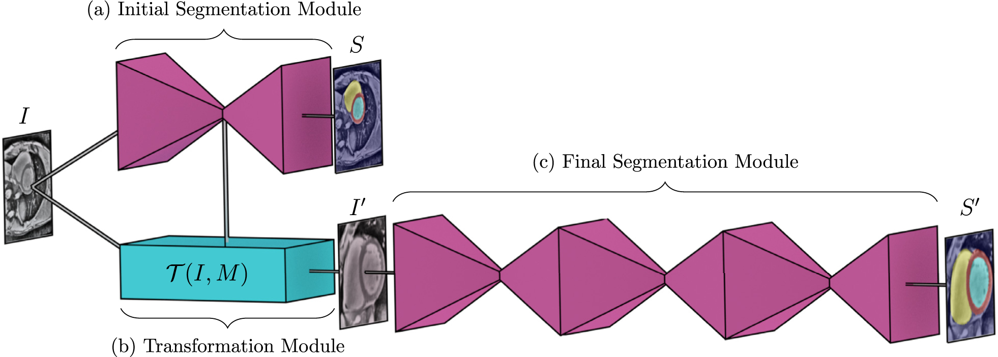
Overview of the Ω-Net architecture (a) The initial, unoriented SSFP image I is fed into a U-Net module, producing an initial segmentation S. (b) The features from the central (most downsampled) layers of this U-Net are used by the transformation module to predict the parameters M of a transformation and transform the input image into a cannonical orientation, . (C) This transformed image is fed into a stacked hourglass module to obtain a final segmentation in the canonical orientation S′. Note that, all modules shown are trained in an end-to-end way from scratch.
For simplicity, we use the U-Net as the fundamental component of the initial and final segmentation modules (Ronneberger et al., 2015), though more advanced networks such as ResNet (He et al., 2016) could be substituted instead. Inspired by the spatial transformer network (Jaderberg et al., 2015), we designed a fully differentiable architecture that simultaneously achieves localization and transformation into a canonical orientation.
The transformed image is then fed into a final segmentation module, which resembles the stacked hourglass architecture (Newell et al., 2016). In a stacked hourglass, segmentation is performed by stacking two or more U-Net-like modules in series, where the features learned by one U-Net serve as the input to its successor, and intermediate segmentations are predicted at the output of each U-Net. This architecture has been shown to produce progressively more accurate predictions, with diminishing returns at each stage (Newell et al., 2016).
We demonstrate that the Ω-Net is capable of the fully automatic segmentation of five foreground classes (LV myocardium, the left and right atria, and the left and right ventricles) in three orthogonal clinical planes (short axis, SA; four-chamber, 4C; and two-chamber, 2C), with simultaneous transformation of the input into a canonical orientation (defined separately for each view, Fig. 2). Moreover, the network is trained on a multicenter population (Ho et al., 2017) of patients with hypertrophic cardiomyopathy (HCM), which increases the complexity of the problem due to the highly variable appearance of the LV in these patients. Network performance as measured by weighted foreground intersection-over-union (IoU) was substantially improved in the best-performing Ω-Net compared with U-Net segmentation without localization and orientation alignment (0.858 vs 0.834). In addition, we retrained the network from scratch on the 2017 MICCAI Automated Cardiac Diagnosis Challenge (ACDC) dataset,1 and achieved results which outperform the current state-of-the-art (Isensee et al., 2018) in terms of LV and RV cavity segmentation, and perform slightly worse in terms of LV myocardium segmentation.
Fig. 2.
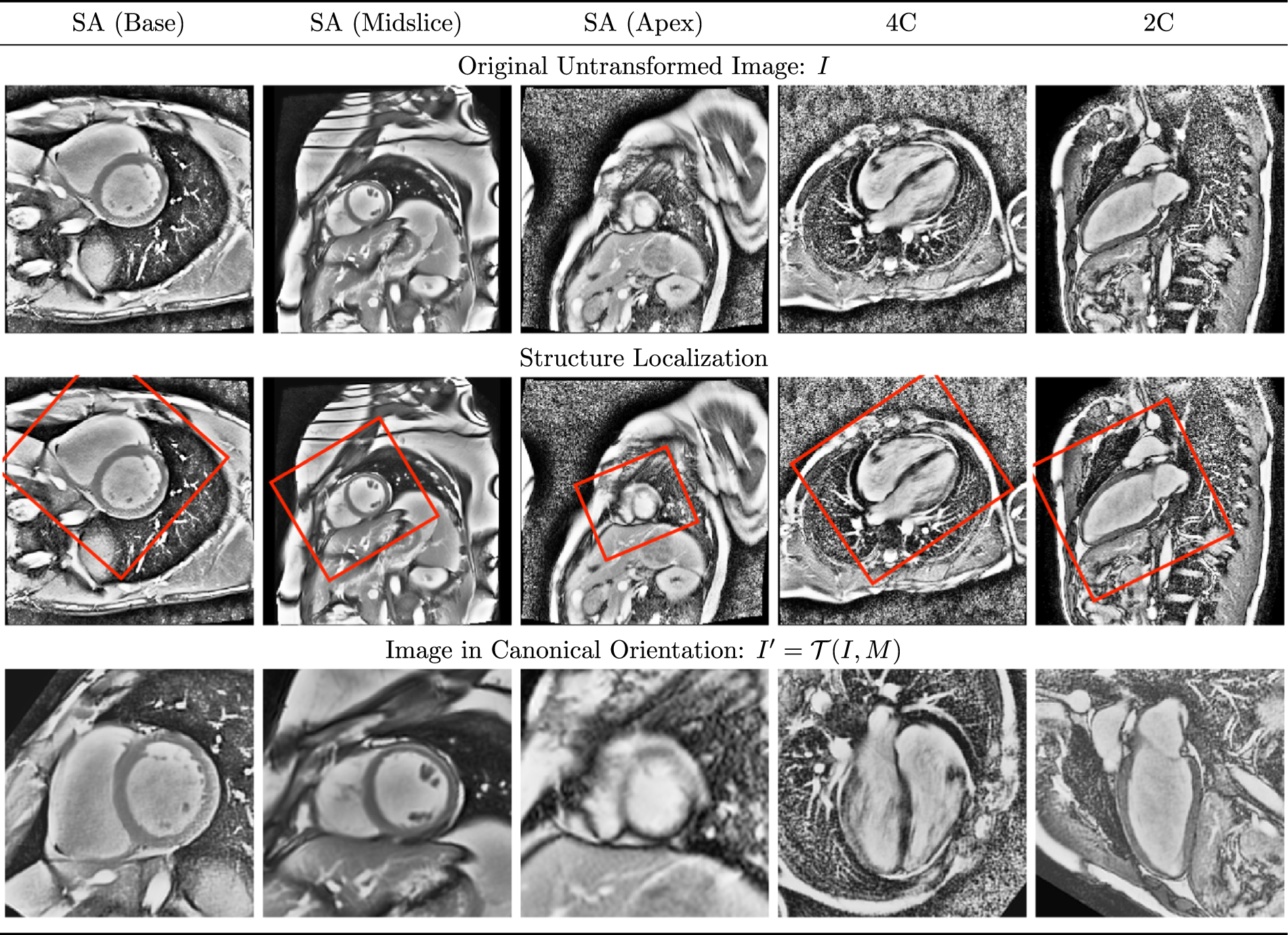
Orthogonal clinical views in canonical orientation Representative short axis (SA), four-chamber (4C), and two-chamber (2C) images are shown as acquired (top), and having undergone transformation into a canonical orientation (bottom). Consistent with common clinical practice, the heart is rotated such that in the SA views, the right ventricle appears on the (radiological) right side of the image, whereas in the 4C and 2C views, the long axis of the left ventricle is oriented vertically. The heart is also centered and scaled to fill 90% of the image. Note the heterogeneity in size, orientation, and appearance of the heart in the untransformed images, which contributes to the difficulty of segmentation.
2. Methods
Due to the lack of rotation invariance/equivariance in CNNs, current practice is for models to be trained with large datasets representing all possible rotations and/or substantial data augmentations (e.g., affine transformations, warpings, etc). We conjecture that biomedical image segmentation can be more efficiently accomplished if structures of interest have first been detected and transformed into a canonical orientation. In the context of CMR, the canonical orientation is defined separately for each clinical plane (Fig. 2). We propose a stepwise strategy for segmentation of cardiac SSFP images in an end-to-end differentiable CNN frame-work, allowing for the localization, alignment, and segmentation tasks to be codependent. Our model consists of three stages. First, the full-resolution, original input image I undergoes an initial segmentation using a U-Net module (Section 2.1). Second, the central (most down-sampled) features of the aforementioned U-Net module are used to predict a matrix M capable of transforming I into a canonical orientation (Section 2.2). Third, the transformed image I′ is segmented using a stacked hourglass module (Section 2.3). In the following subsections, each component of the network is discussed in detail. In terms of notation, a superposed chevron (e.g., ) indicates ground truth, and a superscript tick (e.g., x′ indicates that the quantity pertains to the transformed data.
2.1. Initial segmentation (U-Net) module
The proposed network makes use of the U-Net module (Fig. 3), a type of deep convolutional neural network which has performed well in biomedical segmentation tasks (Long et al., 2015; Ronneberger et al., 2015; Xie et al., 2015). The U-Net architecture consists of a down-sampling path (left) followed by an upsampling path (right) to restore the original spatial resolution. The downsampling path resembles the canonical classification CNN (Krizhevsky et al., 2012; Simonyan and Zisserman, 2014), with two 3 × 3 convolutions, a rectified linear unit (ReLU) activation, and a 2 × 2 max pooling step repeatedly applied to the input image and feature maps. In the upsampling path, the reduction in spatial resolution is “undone” by performing 2 × 2 up-sampling, ReLU activation, and 3 × 3 convolution, eventually mapping the intermediate feature representation back to the original resolution. To provide accurate boundary localization, skip connections are used, where feature representations from the down-sampling path are concatenated with feature maps of the same resolution in the up-sampling path. Batch normalization (Ioffe and Szegedy, 2015), which has been shown to counteract gradient vanishing and to lead to better convergence, was performed between each pair of convolution and ReLU activation layers. The loss for the U-Net module is the categorical cross entropy between the output of the softmax layer, P, and the ground truth segmentation, ,
| (1) |
where
| (2) |
Fig. 3.
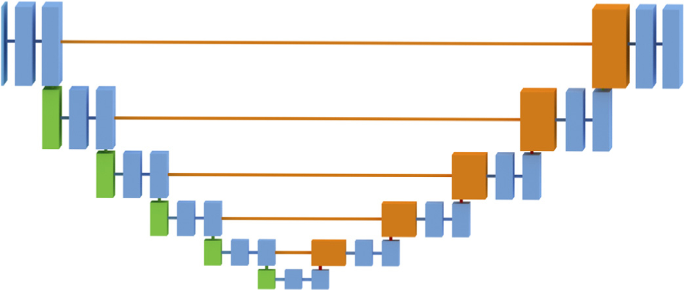
U-Net module The input image is of size 256 × 256 × N, where N is the number of channels (1 for all networks). Blue, green, and orange boxes correspond to multichannel feature maps. Green indicates a downsampled feature map. Orange indicates the result of a copy, concatenated with an upsampled feature map.
Here, H and W are the height and width of the input image in pixels, and h and w are corresponding pixel indices.
2.2. Transformation module
The spatial transformer network (STN) was originally proposed as a general layer for classification tasks requiring spatial invariance for high performance (Jaderberg et al., 2015). The STN module itself consists of three submodules, namely: a localization network (LocNet), which predicts a transformation matrix, M; a grid generator, which implements the transform, ; and a sampler, which implements the interpolation.
In (Jaderberg et al., 2015), the STN was allowed to learn whichever transformation parameters best aid the classification task; no ground truth transformation was specified, and the predicted transformation matrix was used to transform the intermediate feature maps. By contrast, in our application we are specifically interested in learning to transform the input image into the standard clinical orientation, as a precursor to semantic segmentation.
2.2.1. Localization network (LocNet)
Intuitively, a human expert is able to provide translation, rotation, and scaling information given a rough segmentation of the heart. Based on this assumption, we branch out a small localization network (LocNet) from the layer immediately following the final max pooling step of the U-Net in order to predict the transformation parameters (Fig. 4). As we have restricted our transform to allow only translation, rotation, and scaling, the affine matrix was decomposed into three separate matrices:
where T is the translation matrix:
Fig. 4.
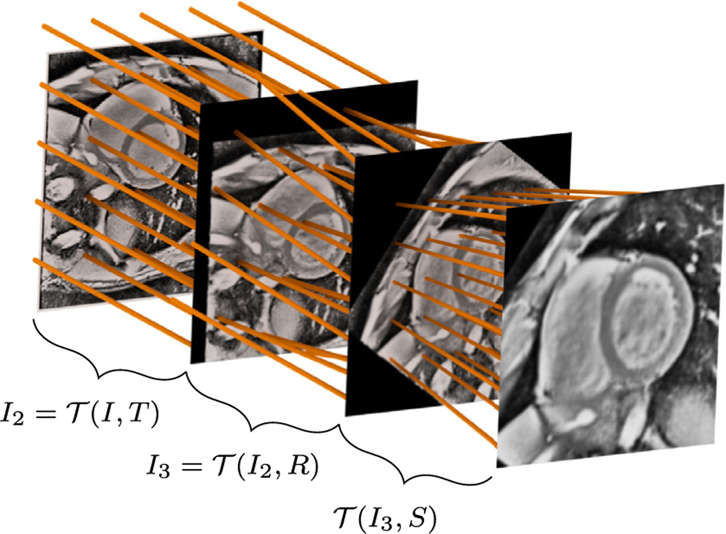
Spatial transformer network module Note that in the actual implementation, all transformations are performed relative to the input image I (i.e., , , and ); for clarity, the transformations have been presented here as successive steps.
R is the (counter clockwise) rotation matrix:
and S is the (uniform) scaling matrix:
Note that the images are defined on a normalized coordinate space {x, y} ∈ [−1, +1], such that rotation and scaling occur relative to the image center.
In practice, the LocNet learns to predict only the relevant parameters, . During training, we explicitly provide the ground-truth transformation parameters , minimizing two types of losses, which we term matrix losses and image losses.
The matrix losses are regression losses between the ground truth and predicted parameters . For scaling and translation, mean squared error (MSE) was used:
| (3) |
| (4) |
| (5) |
Naïve MSE is an inappropriate loss for regressing on θ given its periodicity. Intuitively, this can be understood by considering ground truth and predicted rotations of and θ = −π, which yield a high MSE in spite of being synonymous. For this reason, we introduce a wrapped phase loss, mean squared wrapped error (MSWE, Fig. 5), where is wrapped into the range [−π, π) prior to calculating the standard MSE,
| (6) |
and the wrapping operator is defined as
Fig. 5.
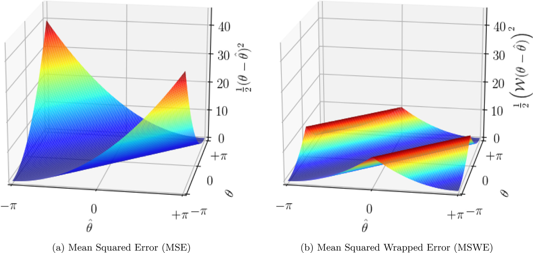
Mean squared error (MSE) vs mean squared wrapped error (MSWE).
Training the transformation module based on these losses alone caused the network to overfit the training data. For this reason, we additionally regularized based on the MSE between the input image after translation, rotation, and scaling with the ground truth and predicted (m) transformation parameters:
| (7) |
| (8) |
| (9) |
2.2.2. Grid generation and sampling
In general, a 2-D “grid generator” takes a (typically uniform) sampling of points and transforms them according to the parameters predicted by a LocNet. In our application, we created three such grids, each of equal dimension to the input H′ = W′ = 256 and uniformly spaced over the extent of the image (x ∈ [−1, 1], y ∈ [−1, 1]). These grids were then transformed by the matrices T, RT, and SRT (predicted by the LocNet) to determine which points to sample from the input image.
The “sampler” takes the input image and the transformed grid G′ as arguments, and produces a resampled image .2 For each channel c ∈ [1 .. C], the output at the location (h′, w′) is a weighted sum of the input values Ih,w,c in the neighborhood of location ,
where
Every step here is differentiable (either a gradient or sub-gradient is defined), such that the model can be trained end-to-end.
2.3. Final segmentation (stacked hourglass) module
The output of the transformation module, having been transformed into a canonical orientation, is then input into a stacked hourglass architecture. The hourglass consisted of D = [1..3] U-Net modules in series with one another, each producing a segmentation SH, d, where d ∈ [1.D]. With reference to Eq. (2), the categorical cross-entropy between the softmax output of the hourglass at depth and the (transformed) ground truth segmentations is calculated,
| (10) |
2.3.1. Summary
To summarize, we train the Ω-Net with one loss from the initial segmentation module, Eq. (1); four matrix losses, Eqs. (3)–(6), and three image losses, Eqs. (7)–(9) from the transformation module; and between one and three losses from the final segmentation module, Eq. (10). Therefore, the overall loss function may be written:
| (11) |
where α1 = 100. 0, α2 = 100. 0, α3 = 0. 1, and α4 = 1. 0. The architectures evaluated are summarized in Table 1.
Table 1.
CNN architecture variants considered. Network A is the baseline U-Net (the initial segmentation module alone, without transformation or final segmentation modules). Networks B, C, and D are full Ω-Net architectures with 1, 2, and 3 U-Net components, respectively, in the fine-grained segmentation module. U-Net 0 is the U-Net in the initial segmentation module; U-Nets 1, 2, and 3 are the first, second, and third U-Net components in the final segmentation module, as applicable. For each U-Net component of each network variant, the length of the feature vector is provided.
| Name | U-Net 0 | U-Net 1 | U-Net 2 | U-Net 3 | Millions of parameters |
|---|---|---|---|---|---|
| Network A | 128 | – | – | – | 7.0 |
| Network B | 64 | 64 | – | – | 3.5 |
| Network C | 64 | 64 | 64 | – | 4.5 |
| Network D | 64 | 64 | 64 | 64 | 5.5 |
While the dataset was manually augmented by transforming the input with small transformations, it is worth noting that data augmentation is performed implicitly in the fine segmentation module by virtue of the fact that, in the early stages of training, the transformation parameters predicted by the transformation module are random.
3. Experiments
3.1. HCMNet dataset
The HCMNet dataset consisted of 63 subjects: 42 patients with overt hypertrophic cardiomyopathy (HCM) and 21 healthy control subjects (Ho et al., 2017). CMR was performed with a standardized protocol at 10 clinical sites from 2009–2011. Nine centers used 1.5-T magnets, and one used a 3-T magnet. Where available, three SA (basal, equatorial, and apical), one 4C, and one 2C SSFP cine series were obtained. Images had an in-plane spacing of 1.3 ± 0.2 mm and matrix size of 253.53 ± 46.73 pixels; further details concerning the CMR acquisition are given in the supplement to Ho et al. (2017).
The LV myocardium, and all four cardiac chambers were manually segmented in the SA, 4C, and 2C views (noting that not all classes are visible in the SA and 2C views). 2-D+time volumes were loaded into ITK-Snap (Yushkevich et al., 2006); every fifth frame was segmented manually, and the remaining frames were automatically interpolated. (Segmentation was performed by the first author, with five years experience in manual CMR segmentation). The papillary muscles and the trabeculation of the LV and RV were excluded from the myocardium.
Each volume was cropped or padded as appropriate to 256 × 256 pixels in the spatial dimensions, and varied from 20–50 frames in the time dimension. Nonuniform background illumination was corrected by dividing by an estimated illumination field, and background corrected images were histogram equalized. Each individual image was normalized to zero mean and unit standard deviation before being input into the CNN.
3.1.1. Training and cross-validation
For cross-validation, the subjects were partitioned into three folds of approximately equal size (4477, 4750, and 4625 images, respectively) such that the images from any one subject were present in one fold only. Each of the four architectures (Table 1) were trained on all three combinations of two folds and tested on the remaining fold. Network A was the initial segmentation module alone; since the U-Net has performed well in biomedical image segmentation tasks, this was regarded as a strong baseline. Networks B, C, and D were Ω-Net architectures with 1, 2, and 3, U-Net components in the final segmentation module.
The networks were initialized with orthogonal weights (Saxe et al., 2014), and were optimized using Adam optimization (Kingma and Ba, 2015) by minimizing categorical cross-entropy. The learning rate was initialized to 0.001 and decayed by 0.1 every 26 epochs. To avoid over-fitting, data augmentation (translations and scaling ± 0.15% of the image width; rotations ± 15°) and a weight decay of 10−4 was applied to the input to the initial segmentation module. Notably, data augmentation is performed implicitly in the final segmentation module, due to the fact that the predicted transformation parameters are random early in training. Note also that data augmentation was performed independently for each time frame.
3.1.2. Measure of performance
Weighted foreground intersection-over-union (IoU) was calculated image-by-image between the prediction and manual segmentations. For a binary image (one foreground class, one background class), IoU (also known as the Jaccard index) is defined for the ground truth and predicted images IT and IP as
| (12) |
noting that a small positive number should be added to the denominator in a practical implementation to avoid division by zero. To extend this concept to multiclass segmentation, IoU was calculated separately for each foreground class. A weighted sum of these five IoU values was then calculated, where the weights were given by the ratio between the relevant foreground class and the union of all foreground classes, yielding weighted, mean foreground IoU.
3.1.3. Implementation
The model was implemented in the Python programming language using the Keras interface to Tensorflow (Chollet, 2015; Abadi et al., 2016), and trained on one NVIDIA Titan X graphics processing unit (GPU) with 12GB of memory. For all network architectures, it took roughly 20 min to iterate over the entire training set (1 epoch). At test time, the network predicted segmentations at roughly 15 frames per second.
3.2. 2017 MICCAI ACDC dataset
Network B was retrained from scratch on the 2017 MICCAI ACDC dataset. This training dataset consists of stacked SA cines from 100 patients with a range of pathologies (20 normal, 20 with myocardial infarction, 20 with dilated cardiomyopathy, 20 with hypertrophic cardiomyopathy, and 20 with RV disease). Ground truth LV myocardium, LV bloodpool, and RV bloodpool segmentations were provided at ED and ES for all spatial slices. Segmentation performance was assessed using both IoU and the Dice coefficient in order to facilitate comparison with the ACDC results:
| (13) |
The network was trained using five-fold cross-validation, in accordance with the current state-of-the-art (Isensee et al., 2017; 2018).
4. Results
4.1. HCMNet dataset
4.1.1. Segmentation
Weighted foreground IoU was calculated separately for each image, and the median and interquartile range (IQR) of all predictions is reported. As accuracy is not necessarily the same across all clinical planes, the performance of the four networks relative to manual segmentation is reported for all views combined, and also for each clinical plane separately (Table 2).
Table 2.
Network performance with reference to ground truth. Weighted foreground IoU for each network variant is calculated for all views combined and for each view separately, and is reported as median [interquartile range]. Network performance was highest in the SA view and lowest in the 4C view, though these differences are small.
| Name | View | U-Net 0 | U-Net 1 | U-Net 2 | U-Net 3 |
|---|---|---|---|---|---|
| Network A | All | 0.834 [0.783, 0.871] | – | – | – |
| SA | 0.843 [0.789, 0.880] | – | – | – | |
| 4C | 0.819 [0.765, 0.855] | – | – | – | |
| 2C | 0.831 [0.788, 0.863] | – | – | – | |
| Network B | All | 0.841 [0.793, 0.876] | 0.857 [0.819, 0.885] | – | – |
| SA | 0.848 [0.800, 0.884] | 0.862 [0.820, 0.891] | – | – | |
| 4C | 0.831 [0.780, 0.861] | 0.845 [0.812, 0.871] | – | – | |
| 2C | 0.832 [0.787, 0.864] | 0.856 [0.822, 0.882] | – | – | |
| Network C | All | 0.841 [0.792, 0.875] | 0.856 [0.816, 0.884] | 0.857 [0.816, 0.885] | – |
| SA | 0.849 [0.797, 0.883] | 0.862 [0.820, 0.890] | 0.862 [0.819, 0.890] | – | |
| 4C | 0.830 [0.779, 0.861] | 0.843 [0.804, 0.869] | 0.844 [0.805, 0.869] | – | |
| 2C | 0.830 [0.793, 0.863] | 0.855 [0.818, 0.883] | 0.857 [0.819, 0.884] | – | |
| Network D | All | 0.844 [0.797, 0.877] | 0.856 [0.819, 0.884] | 0.858 [0.821, 0.886] | 0.858 [0.821, 0.886] |
| SA | 0.851 [0.798, 0.886] | 0.862 [0.821, 0.890] | 0.863 [0.822, 0.892] | 0.863 [0.822, 0.892] | |
| 4C | 0.832 [0.781, 0.861] | 0.839 [0.805, 0.868] | 0.843 [0.811, 0.870] | 0.843 [0.811, 0.869] | |
| 2C | 0.842 [0.804, 0.869] | 0.858 [0.828, 0.884] | 0.860 [0.831, 0.886] | 0.859 [0.830, 0.886] |
It is instructive to examine intermediate network performance at each successive U-Net (Fig. 6).
Although Network A contains the most parameters, adding the final segmentation module was found to increase network performance at the level of the initial U-Net compared with Network A; i.e., the performance of the initial segmentation module U-Net (U-Net 0) is ≈ 0.007 higher in Networks B and C compared with Network A, and ≈ 0.003 higher in Network D compared with Networks B and C.
There was a substantial increase in performance between the initial and final segmentation U-Nets, i.e., U-Nets 0 and 1 (≈ 0.016, ≈ 0.015, and ≈ 0.012 increases for Networks B, C, and D, respectively).
In Networks C and D, there was not a substantial increase in performance between successive U-Nets in the final segmentation module.
Fig. 6.
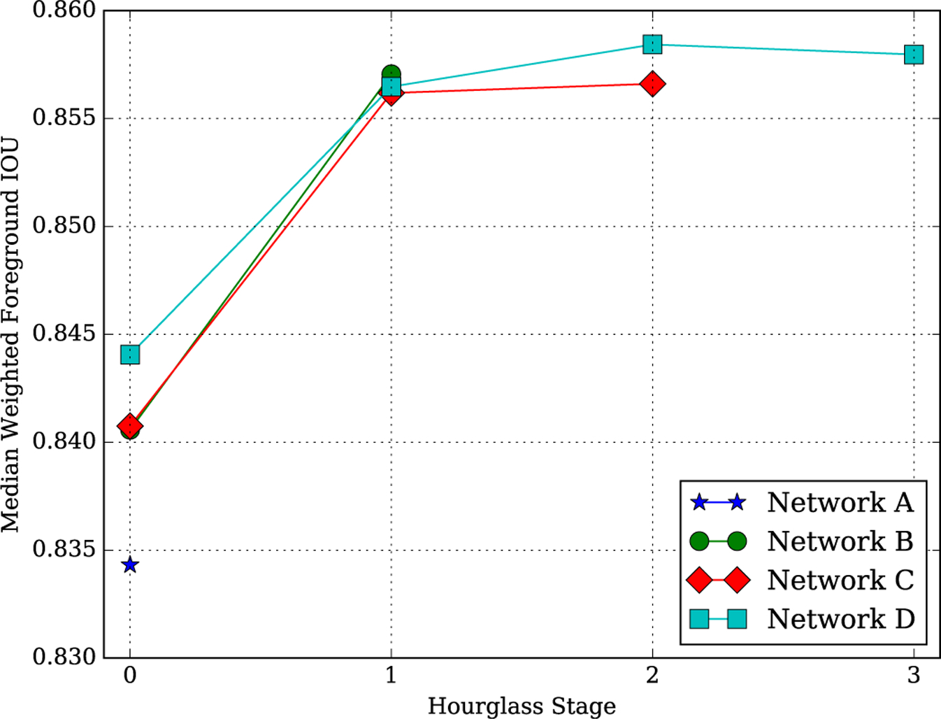
Weighted foreground IoU for architecture and depth.
As performance is likely to differ between structures, image-wise histograms of foreground IoU are plotted for the best performing network (Network D) for each structure and clinical plane (Fig. 7). In all three clinical planes, performance is worst for the LV myocardium, best for the LV blood pool, and intermediate for the remaining structures. Intuitively, relatively poor LV myocardial segmentation performance can be understood by considering that segmentation error is concentrated primarily at the structure boundaries. Therefore, structures with a high ratio of perimeter-to-area (such as the LV myocardium, which has both an internal and external perimeter, i.e., endocardium and epicardium) are predisposed to perform poorly. A number of factors may contribute to the superior performance of LV bloodpool segmentation.
The LV myocardium provides a high-contrast boundary along much of the perimeter of the LV bloodpool.
Compared with other cardiac chambers, the LV bloodpool has relatively less anatomical variation between subjects.
The three orthogonal planes examined in this study are all defined relative to the left ventricle; therefore, the appearance of the LV is more consistent between subjects.
Fig. 7.
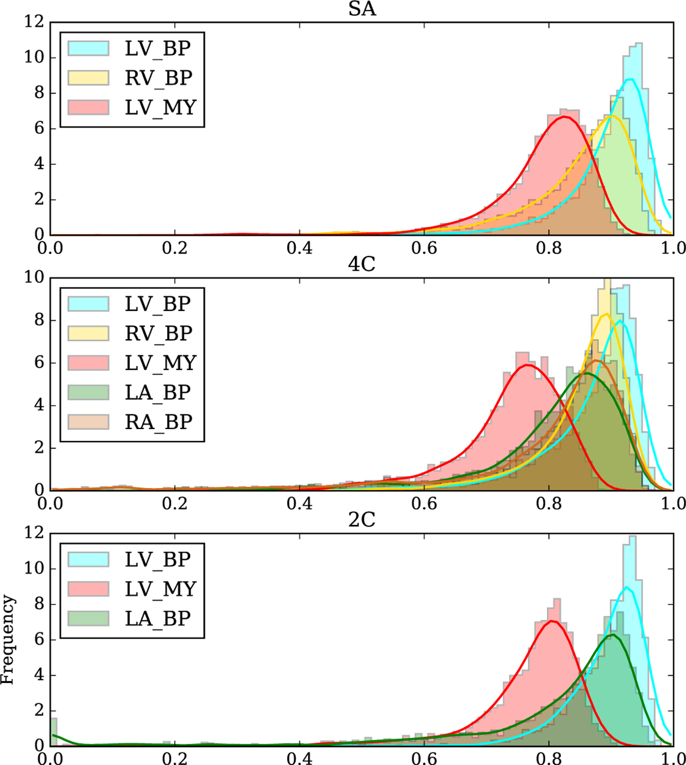
Histograms of IoU for each view and class. Performance relative to manual segmentation was highest in the SA view and lowest in the 4C view, though the differences are small. LV_BP: left ventricular blood pool; RV_BP: right ventricular blood pool; LV_MY: left ventricular myocardium; LA_BP: left atrial blood pool; RA_BP: right atrial blood pool.
Fig. 8 presents the precision-recall curve, showing the “success rate” (vertical axis) defined as the fraction of cases in which weighted foreground IoU exceeded a varying threshold varying from 0.4–1.0 (horizontal axis). The resulting precision-recall curve had an area under the curve (AUC) of 0.992, demonstrating the accuracy of the Ω-Net. The “failure rate” can also be calculated from this curve as 1 - successrate. For example, for a conservative definition of failure as weighted foreground IoU < 0.9, the failure rate is approximately 1%.
Fig. 8.
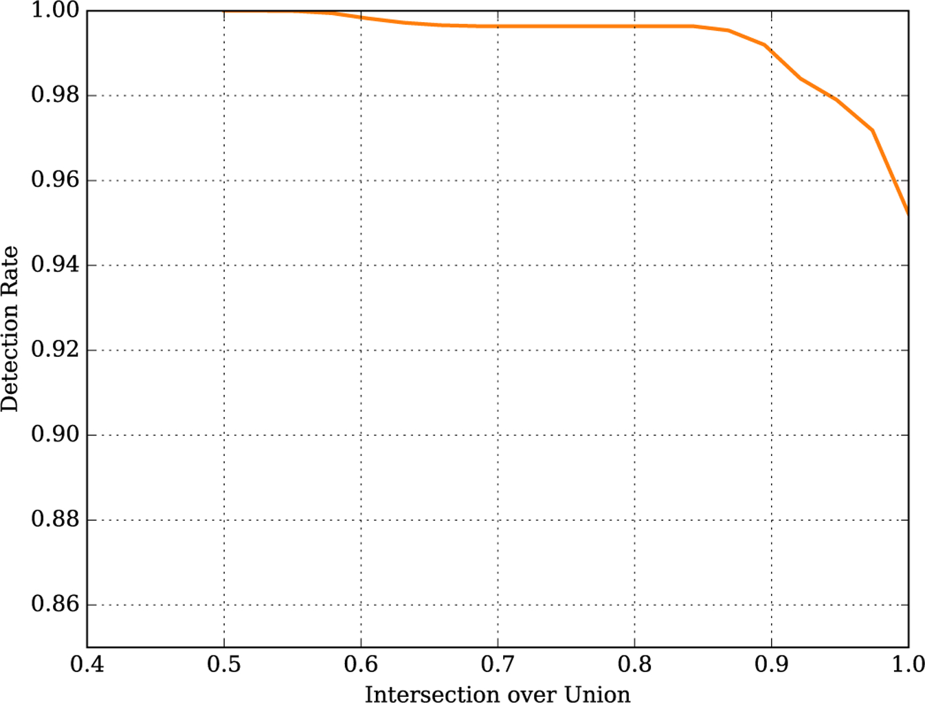
Precision-Recall curve.
Representative segmentations produced by Network D in all views are shown for healthy control subjects in Fig. 9 and for patients with overt HCM in Fig. 10. Note that the ground truth segmentations have been transformed by the predicted parameters rather than the ground truth parameters in order to aid interpretation in these figures. The network successfully transformed the images into the canonical orientation for all cases shown. Notably, the myocardial segmentation consistently excludes papillary muscles and myocardial trabeculation. Moreover, the network appears to reliably identify the atrioventricular valve plane in the long axis views, which is a useful result deserving of attention in future work.
Fig. 9.
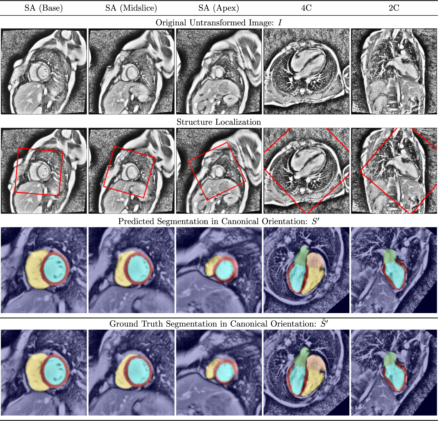
Representative segmentation results in healthy control subjects See text for discussion.
Fig. 10.
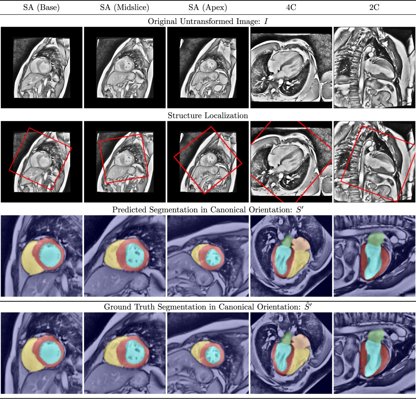
Representative segmentation results in patients with overt HCM. See text for discussion.
4.1.2. Transformation parameters
Ground truth parameters were compared to those predicted by the best performing network (Network D) via correlation, and by Bland Altman plots (Fig. 11). It is notable that ground truth transformation parameters (particularly rotation and scale) were not uniformly distributed between views. Nonrandom rotation is to be expected from the fact that the positioning of the patient in the scanner, the protocol for determining imaging planes, the placement of the heart in the chest, and the relationship between imaging planes are all themselves nonrandom; nonrandom scale is likewise to be expected from the variable size of the anatomical structures visible in each view.
Fig. 11.
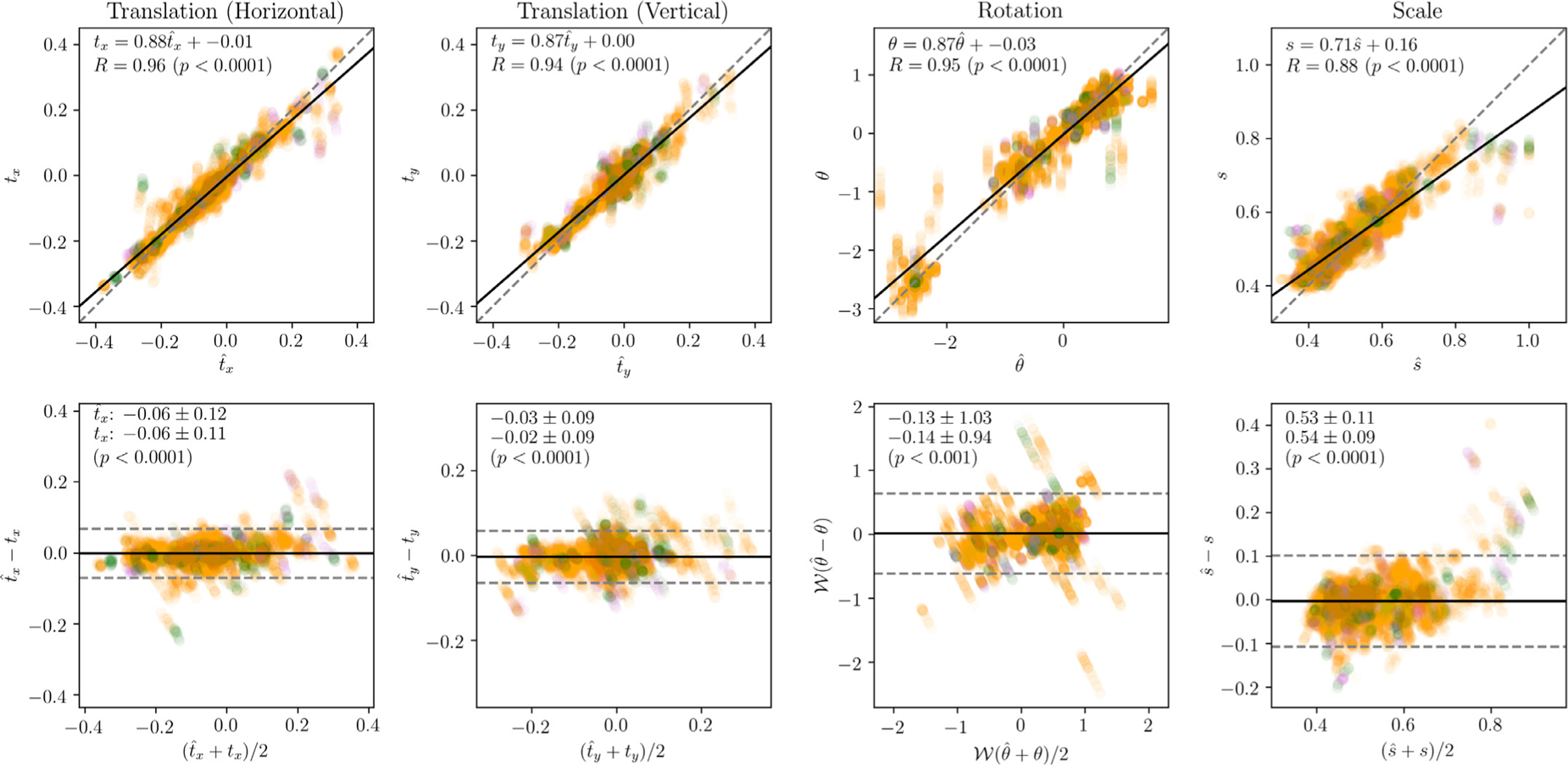
Transformation errors. Correlation (top) and Bland-Altman (bottom) plots comparing predicted and ground truth transformation parameters. SA, 4C, and 2C errors are represented by orange, green, and purple points, respectively (points have been rendered partially translucent to aid interpretation of densely occupied regions). In the correlation plots, the best-fit trendline is represented as a solid black line, and the ideal trendline (y = x) is represented as a dashed, gray line. The equation of the trendline and the Pearson correlation coefficient R are also given. In the Bland-Altman plots, the mean difference is represented as a solid black horizontal line, and the limits ± 1.96 standard deviations are represented as a dashed gray horizontal line.
Predicted horizontal translation, vertical translation, and rotation parameters were all highly correlated with ground truth (R ≈ 0.95, p < 0.0 0 01 for all), with the predicted parameters slightly under-estimating the ground truth (slope ≈ 0.87 for all). Systematic bias was not evident on visual inspection of the Bland-Altman plots; 95% of translation errors were within ± 0.07 (in normalized image coordinates), and 95% of rotation errors were within ± 0.63 (in radians). Of the 5% of cases which were outside these bounds, the vast majority were long axis (4C or 2C) views. This is perhaps not surprising since each patient contributed three SA views, but only two long axis views.
Compared with translation and rotation, correlation between ground truth and predicted scale was slightly lower, though still good (R = 0. 88, p < 0.0 0 01); predicted scale again slightly underestimated ground truth scale . There was a marked decrease in network performance above approximately . This may indicate the importance of context information to the network. However, it should be noted that the decrease in performance is accompanied by a sharp decrease in the frequency of cases, and so may also be the result of an insufficient number of samples in the dataset.
4.1.3. Failure cases
Occasional failure cases were observed, a selection of which are shown in Fig. 12. Each of these failure cases has one or more features which could logically explain the failure. The leftmost column shows an apical SA slice from a severely hypertrophied patient. Patients with such severe disease were relatively uncommon in the dataset, perhaps causing the network to split its attention between the heart and a second “candidate structure” (the cardia of the stomach). The center-left column shows a second apical SA slice from a different subject, where the right ventricle was incorrectly segmented. The signal intensity in this image was low relative to the other patients in the cohort, resulting in a very high contrast image after histogram equalization. The center-right and rightmost columns show long axis views from a patient with a particularly high resolution scan, where the heart occupies the vast majority of the image, with very little context information. In both cases, catastrophic segmentation error follows failure to properly reorient the image into a canonical orientation. However, it should be emphasized that this post hoc reasoning is speculative; we cannot state a definitive causal relationship between these features and the resulting failures.
Fig. 12.
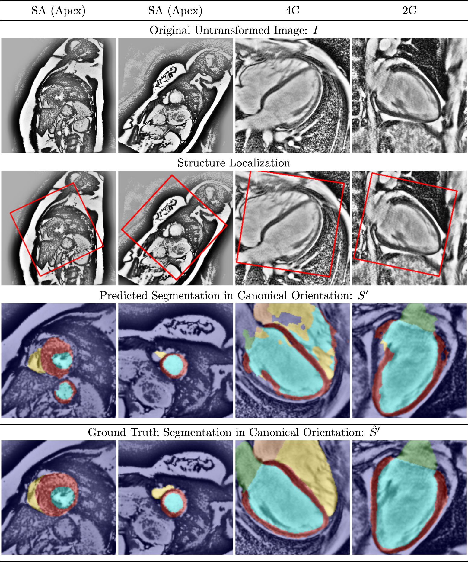
Selected failure cases from CNN segmentation. See text for discussion.
4.2. 2017 MICCAI ACDC dataset
Isensee et al. (2017) represents the state-of-the-art network in terms of segmentation accuracy on the ACDC leaderboard; this same group has since released an unpublished revision3 with improved results (Isensee et al., 2018). To match their methods, we retrained the Network B variant of Ω-Net from scratch using five-fold cross-validation on the provided dataset (each patient only appears in one fold). Single model segmentation accuracy is reported for Ω-Net, Isensee et al. (2017), and Isensee et al. (2018) in Table 3. Compared with Isensee et al. (2017), our results give higher IoU for all foreground classes: LV bloodpool (0.912 vs 0.869), RV bloodpool (0.852 vs 0.784), and LV myocardium (0.803 vs 0.775). Compared with Isensee et al. (2018), our results give higher IoU for LV blood-pool (0.912 vs 0.896) and RV bloodpool (0.852 vs 0.832), but lower IoU for LV myocardium (0.803 vs 0.826).
Table 3.
Segmentation accuracy on the 2017 MICCIA ACDC dataset. Segmentation accuracy is reported as Dice coefficient in the ACDC challenge, but as IoU elsewhere in this work; therefore, both are reported here. (Note that Dice = 2 × IoU/(1 + IoU)). Results are reported for the Network B variant of the Ω-Net; for the results by Isensee et al. (2017) published in STACOM; and for the same group’s unpublished arxiv.org revision Isensee et al. (2018). Boldface formatting indicates the best performing model for each foreground class. MICCAI: Medical Image Computing and Computer Assisted Intervention Society; ACDC: Automated Cardiac Diagnosis Challenge.
| Structure | LV Bloodpool | RV Bloodpool | LV Myocardium |
|---|---|---|---|
| Jaccard index (IoU) | |||
| Ω-Net | 0.912 | 0.852 | 0.803 |
| Isensee et al. (2018) | 0.896 | 0.832 | 0.826 |
| Isensee et al. (2017) | 0.869 | 0.784 | 0.775 |
| Dice coefficient | |||
| Ω-Net | 0.954 | 0.920 | 0.891 |
| Isensee et al. (2018) | 0.945 | 0.908 | 0.905 |
| Isensee et al. (2017) | 0.930 | 0.879 | 0.873 |
5. Discussion
In this work, we have presented the Ω-Net: A novel deep convolutional neural network (CNN) architecture for localization, orientation alignment, and segmentation. We have applied this network to the task of fully automatic whole-heart segmentation and simultaneous transformation into the “canonical” clinical view, which has the potential to greatly simplify downstream analyses of SSFP CMR images. The network was trained end-to-end from scratch to segment five foreground classes (the four cardiac chambers plus the LV myocardium) in three views (SA, 4C, and 2C), without providing prior knowledge of the view being segmented. The dataset was highly heterogeneous from the standpoint of anatomical variation, including both healthy subjects and patients with overt hypertrophic cardiomyopathy. Data was acquired from both 1.5-T and 3-T magnets as part of a multicenter trial involving 10 institutions. In cross-validation experiments, the network performed well in predicting both the parameters of the transformation, and the cardiac segmentation.
Ω-Net also achieved state-of-the-art performance on the publicly available 2017 MICCAI ACDC dataset in two of three classes. Compared with our internal HCMNet dataset, ACDC contains a broader range of LV and RV pathologies, but only one clinical view, and fewer foreground classes. Moreover, HCMNet was a multicenter study, whereas ACDC was acquired at a single center. It is encouraging that Ω-Net performed well on both datasets.
The prior state-of-the-art (Isensee et al., 2017; 2018) was achieved using an ensemble of 2D and 3D U-Net-inspired architectures, optimized for stacked cine series. Their method is therefore not generally applicable to 4C and 2C views, which are typically acquired as single slices. Therefore, Ω-Net outperformed Isensee et al. (2018) while remaining more general, and while providing localization and orientation information not predicted by (Isensee et al., 2017).
The work is novel in four principal ways. First, this network predicts five foreground classes in three clinical views, which is a substantially more difficult problem than has been addressed previously in the literature (Vigneault et al., 2017). Second, a spatial transformer network module (Jaderberg et al., 2015) was used to rotate each view into a canonical orientation. CNNs are neither rotation invariant nor equivariant, nor scale invariant. From a technical standpoint, in theory this shortcoming can be addressed by acquiring very large datasets which adequately represent all possible rotations. However, biomedical imaging datasets are expensive and time consuming both to acquire and to annotate, directly motivating this design decision. By standardizing the orientation of the input to the final segmentation module, we simplify the task of both the downstream network and the physician interpreting the images. Third, the proposed architecture takes loose inspiration from the cascaded classifier models proposed by Viola and Jones (2001), in that U-Net 0 performs initial segmentation (in order to predict transformation parameters), and the transformed image is then provided as input to a final segmentation module (U-Nets 1, 2, and 3). Last, by its design, Ω-Net provides human-interpretable, intermediate outputs (an initial segmentation and transformation parameters) in addition to the final segmentation. In doing so, we substantially increase the complexity and information predicted by the network compared to the U-Net architecture, but without adding concerns that CNNs are “black boxes” whose internals cannot be adequately interrogated.
Although the dataset included three orthogonal cardiac planes and both healthy subjects and those with LV pathology, there remain potential opportunities to extend the dataset to more general scenarios. First, other cardiac planes used in clinical practice (such as the axial, three-chamber, and RV long axis views) should be added in future work. It would also be useful and interesting to test this on other CMR pulse sequences (such as gradient echo) and on additional modalities (i.e., cardiac computed tomography and echocardiography). Difficulty generalizing beyond the clinical views, pulse sequences, pathologies, and variable cardiac geometries represented in the training dataset is a limitation common to all neural networks (and, indeed, to any model governed by Bayesean statistics). Although the Ω-Net, trained through cross-validation, performed well in both multi-center (HCMNet) and multi-pathology (ACDC) datasets (trained from scratch in each case), it would be interesting in future work to study the performance of a model trained on one dataset and tested on an entirely different dataset, with and without fine-tuning. Moreover, it could also be interesting to apply this technique to other areas within biomedical image segmentation where localization, reorientation, and segmentation are useful, such as in fetal imaging. Finally, we expect Ω-Net to be useful in applications requiring the segmentation of multiple clinical planes, such as CMR motion correction and slice alignment (Sinclair et al., 2017).
A variety of opportunities present themselves in terms of optimizing the Ω-Net architecture. For example, the network was trained to segment individual image frames, without spatial or temporal context; modifying the architecture to allow information sharing between temporal frames and spatial slices has the potential to increase accuracy and consistency. The E-Net (“Efficient Net”) provides modifications to the U-Net blocks which increase computational and memory efficiency, while preserving accuracy (Paszke et al., 2016); these lessons have been applied successfully to cardiac segmentation (Lieman-Sifry et al., 2017), and could the-oretically be applied here as well.
6. Summary
We have presented Ω-Net (Omega-Net): A novel CNN architecture for simultaneous localization, transformation into a canonical orientation, and semantic segmentation. First, an initial segmentation is performed on the input image; second, the features learned during this initial segmentation are used to predict the parameters needed to transform the input image into a canonical orientation; and third, a final segmentation is performed on the transformed image. The network was trained end-to-end from scratch on two different datasets. On the HCMNet dataset, Ω-Net was trained to predict five foreground classes in three clinical views, constituting a substantially more challenging problem compared with prior work. The trained network performed well in a cohort of both healthy subjects and patients with severe LV pathology. A variant of the Ω-Net network was trained from scratch on a publicly-available dataset, and achieved state-of-the-art performance in two of three segmentation classes. We believe this architecture represents a substantive advancement over prior approaches, with implications for biomedical image segmentation more generally.
Acknowledgements
D.M. Vigneault is supported by the NIH-Oxford Scholars Program and the NIH Intramural Research Program. W. Xie is supported by the Google DeepMind Scholarship, and the EPSRC Programme Grant Seebibyte EP/M013774/1.
Footnotes
Supplementary material
Supplementary material associated with this article can be found, in the online version, at 10.1016/j.media.2018.05.008.
For completeness, we have included the number of channels C in this description as a variable parameter; however, it should be emphasized that in our application the grayscale input image I is transformed, such that C = 1.
References
- Abadi M, Barham P, Chen J, Chen Z, Davis A, Dean J, Devin M, Ghemawat S, Irving G, Isard M, Kudlur M, Levenberg J, Monga R, Moore S, Murray DG, Steiner B, Tucker P, Vasudevan V, Warden P, Wicke M, Yu Y, Zheng X, 2016. Tensorflow: a system for large-scale machine learning. https://arxiv.org/pdf/1605.08695.pdf. arXiv:1605.08695v2.
- Chollet F, 2015. Keras. https://github.com/fchollet/keras.
- Dieleman S, Willett KW, Dambre J, 2015. Rotation-invariant convolutional neural networks for galaxy morphology prediction. Mon. Not. R. Astron. Soc 450 (2), 1441–1459. doi: 10.1093/mnras/stv632. ArXiv:1503.07077 [DOI] [Google Scholar]
- He K, Zhang X, Ren S, Sun J, 2016. Deep Residual Learning for Image Recognition. CVPR. ArXiv:1512.03385v1 [Google Scholar]
- Ho CY, Day SM, Colan SD, Russell MW, Towbin JA, Sherrid MV, Canter CE, Jefferies JL, Murphy AM, Cirino AL, Abraham TP, Taylor M, Mestroni L, Bluemke DA, Jarolim P, Shi L, Sleeper LA, Seidman CE, Orav EJ, 2017. The burden of early phenotypes and the influence of wall thickness in hypertrophic cardiomyopathy mutation carriers. JAMA Cardiol. 2 (4), 419–428. doi: 10.1001/jamacardio.2016.5670. http://cardiology.jamanetwork.com/article [DOI] [PMC free article] [PubMed] [Google Scholar]
- Ioffe S, Szegedy C, 2015. Batch Normalization: Accelerating Deep Network Training by Reducing Internal Covariate Shift. In: ICML, Vol. 37, pp. 81–87. doi: 10.1007/s13398-014-0173-7.2. http://arxiv.org/abs/1502.03167. arXiv:1011.1669v3 [DOI] [Google Scholar]
- Isensee F, Jaeger P, Full PM, Wolf I, Engelhardt S, Maier-Hein KH, 2017. Automatic Cardiac Disease Assessment on Cine-MRI via Time-series Segmentation and Domain Specific Features. STACOM; Quebec City, Quebec, Canada [Google Scholar]
- Isensee F, Jaeger P, Full PM, Wolf I, Engelhardt S, Maier-Hein KH, 2018. Automatic cardiac disease assessment on cine-MRI via time-series segmentation and domain specific features. http://arxiv.org/abs/1707.00587. arXiv:1707.00587.
- Jaderberg M, Simonyan K, Zisserman A, Kavukcuoglu K, 2015. Spatial Transformer Networks. In: NIPS, pp. 1–14. doi: 10.1038/nbt.3343. ArXiv:1506.02025v1 [DOI] [Google Scholar]
- Kingma D, Ba J, 2015. Adam: a method for stochastic optimization. ICLR. ArXiv:1412.6980v9 [Google Scholar]
- Krizhevsky A, Sutskever I, Hinton GE, 2012. Imagenet Classification with Deep Convolutional Neural Networks. NIPS. [Google Scholar]
- Lieman-Sifry J, Le M, Lau F, Sall S, Golden D, 2017. Fastventricle: Cardiac Segmentation with ENet. FIMH. http://arxiv.org/abs/1704.04296.arXiv:1704.04296 [Google Scholar]
- Long J, Shelhamer E, Darrell T, 2015. Fully Convolutional Networks for Semantic Segmentation. In: CVPR, Vol. 07–12-June, pp. 3431–3440. doi: 10.1109/CVPR.2015.7298965. ArXiv:1411.4038 [DOI] [PubMed] [Google Scholar]
- Luo G, An R, Wang K, Dong S, Zhang H, 2016. A deep learning network for right ventricle segmentation in short-axis MRI. Comput. Cardiol 43, 485–488. [Google Scholar]
- Newell A, Yang K, Deng J, 2016. Stacked Hourglass Networks for Human Pose Estimation. ECCV doi: 10.1007/978-3-319-46484-8. http://arxiv.org/abs/1603.06937 arXiv:1603.06937 [DOI] [Google Scholar]
- Noh H, Hong S, Han B, 2015. Learning Deconvolution Network for Semantic Segmentation. ICCV, Vol. 1 doi: 10.1109/ICCV.2015.178. http://arxiv.org/abs/1505.04366 arXiv:1505.04366 [DOI] [Google Scholar]
- Paszke A, Chaurasia A, Kim S, Culurciello E, 2016. ENet: A deep neural network architecture for real-time semantic segmentation. https://arxiv.org/abs/1606.02147. arXiv:1606.02147v1.
- Peng P, Lekadir K, Gooya A, Shao L, Petersen SE, Frangi AF, 2016. A review of heart chamber segmentation for structural and functional analysis using cardiac magnetic resonance imaging. MAGMA 29 (2), 155–195. doi: 10.1007/s10334-015-0521-4. [DOI] [PMC free article] [PubMed] [Google Scholar]
- Poudel RP, Lamata P, Montana G, 2016. Recurrent Fully Convolutional Neural Networks for Multi-slice MRI Cardiac Segmentation. HVSMR doi: 10.1007/978-3-319-52280-7_8. http://arxiv.org/abs/1608.03974 arXiv:1608.03974 [DOI] [Google Scholar]
- Ronneberger O, Fischer P, Brox T, 2015. U-net: Convolutional Networks for Biomedical Image Segmentation. In: MICCAI, pp. 234–241. doi: 10.1007/978-3-319-24574-4_28. ArXiv:1505.04597 [DOI] [Google Scholar]
- Saxe AM, McClelland JL, Ganguli S, 2014. Exact Solutions to the Nonlinear Dynamics of Learning in Deep Linear Neural Networks. In: ICLR, pp. 1–22. http://arxiv.org/abs/1312.6120 arXiv:1312.6120 [Google Scholar]
- Sifre L, Mallat S, 2013. Rotation, scaling and deformation invariant scattering for texture discrimination. Proc. IEEE Comput. Soc. Conf. Comput. Vis. Pattern Recognit 1233–1240. doi: 10.1109/CVPR.2013.163. [DOI] [Google Scholar]
- Simonyan K, Zisserman A, 2014. Very Deep Convolutional Networks for Large-scale Image Recognition. In: ICLR, pp. 1–14. ArXiv:1409.1556v6 [Google Scholar]
- Sinclair M, Bai W, Puyol-Antón E, Oktay O, Rueckert D, King AP, 2017. Fully Automated Segmentation-based Respiratory Motion Correction of Multi-planar Cardiac Magnetic Resonance Images for Large-scale Datasets. In: MICCAI, Vol. 2, pp. 332–340. doi: 10.1007/978-3-319-66185-8_38. http://link.springer.com/10.1007/978-3-319-66185-8_38 [DOI] [Google Scholar]
- Tan LK, Liew YM, Lim E, Mclaughlin RA, 2016. Cardiac Left Ventricle Segmentation Using Convolutional Neural Network Regression. In: IECBES, pp. 490–493. [Google Scholar]
- Tan LK, Liew YM, Lim E, McLaughlin RA, 2017. Convolutional neural network regression for short-axis left ventricle segmentation in cardiac cine MR sequences. Med. Image Anal 39, 78–86. doi: 10.1016/j.media.2017.04.002. https://www.sciencedirect.com/science/article/pii/S1361841517300543 [DOI] [PubMed] [Google Scholar]
- Tran PV, 2016. A fully convolutional neural network for cardiac segmentation in short-axis MRI. http://arxiv.org/abs/1604.00494 arXiv:1604.00494.
- Vigneault D, Xie W, Bluemke D, Noble J, 2017. Feature tracking cardiac magnetic resonance via deep learning and spline optimization. volume 10263 LNCS, 10.1007/978-3-319-59448-4_18. [DOI] [Google Scholar]
- Viola P, Jones M, 2001. Rapid Object Detection Using a Boosted Cascade of Simple Features. CVPR. [Google Scholar]
- Xie W, Noble JA, Zisserman A, 2015. Microscopy Cell Counting with Fully Convolutional Regression Networks. In: MICCAI Workshop, pp. 1–10. doi: 10.1080/21681163.2016.1149104. [DOI] [Google Scholar]
- Yu F, Koltun V, 2016. Multi-scale Context Aggregation by Dilated Convolutions. In: ICLR, pp. 1–9. doi: 10.16373/j.cnki.ahr.150049. http://arxiv.org/abs/1511.07122 arXiv:1511.07122 [DOI] [Google Scholar]
- Yushkevich PA, Piven J, Hazlett HC, Smith RG, Ho S, Gee JC, Gerig G, 2006. User-guided 3d active contour segmentation of anatomical structures : significantly improved efficiency and reliability. Neuroimage 31, 1116–1128. doi: 10.1016/j.neuroimage.2006.01.015. [DOI] [PubMed] [Google Scholar]


